Source Separation and Identication issues in bio signals:
A solution using Blind source separation 69

6.2 Limitations

The results on facial sEMG analysis demonstrated that, the proposed method provides
interesting result for inter experimental variations in facial muscle activity during different
vowel utterance. The accuracy of recognition is poor when the system is used for testing the
training network for all subjects. This shows large variations between subjects (inter-subject
variation) because of different style and speed of speaking. This method has only been
tested for limited vowels. This is because the muscle contraction during the utterance of
vowels is relatively stationary while during consonants there are greater temporal
variations.

The results demonstrate that for such a system to succeed, the system needs to be improved.
Some of the possible improvements that the authors suggest will include improved
electrodes, site preparation, electrode location, and signal segmentation. This current
method also has to be enhanced for large set of data with many subjects in future. The
authors would like to use this method for checking the inter day and inter experimental
variations of facial muscle activity for speech recognition in near future to test the reliability
of ICA for facial SEMG

7. Conclusions
BSS technique has been considered for decomposing sEMG to obtain the individual muscle
activities. This paper has proposed the applications and limitations of ICA on hand gesture
actions and vowel utterance.

A semi blind source separation using the prior knowledge of the biological model of sEMG
had been used to test the reliability of the system. The technique is based on separating the
muscle activity from sEMG recordings, saving the estimated mixing matrix, training the
neural network based classifier for the gestures based on the separated muscle activity, and

subsequently using the combination of the mixing matrix and network weights to classify
the sEMG recordings in near real-time.

The results on hand gesture identification indicate that the system is able to perfectly (100%
accuracy) identify the set of selected complex hand gestures for each of the subjects. These
gestures represent a complex set of muscle activation and can be extrapolated for a larger
number of gestures. Nevertheless, it is important to test the technique for more actions and
gestures, and for a large group of people.

The results on vowel classification using facial sEMG indicate that while there is a similarity
between the muscle activities, there are inter-experimental variations. There are two
possible reasons; (i) people use different muscles even when they make the same sound and
(ii) cross talk due to different muscles makes the signal quality difficult to classify
Normalisation of the data reduced the variation of magnitude of facial SEMG between
different experiments. The work indicates that people use same set of muscles for same
utterances, but there is a variation in muscle activities. It can be used a preliminary analysis

for using Facial SEMG based speech recognition in applications in Human Computer
Interface (HCI).

8. References
Attias, H. & Schreiner, C. E. (1998). Blind source separation and deconvolution: the dynamic
component analysis algorithm, Neural Comput. Vol. 10, No. 6, 1373–1424.
Azzerboni, B. Carpentieri, M. La Foresta, F. & Morabito, F. C. (2004), Neural-ica and wavelet
transform for artifacts removal in surface emg, Proceedings of IEEE International Joint
Conference’, pp. 3223–3228, 2004.
Azzerboni, B. Finocchio, G. Ipsale, M. La Foresta, F. Mckeown, M. J. & Morabito, F. C.
(2002). Spatio-temporal analysis of surface electromyography signals by
independent component and time-scale analysis, in Proceedings of 24th Annual
Conference and the Annual Fall Meeting of the Biomedical Engineering Society

EMBS/BMES Conference, pp. 112–113, 2002.
Barlow, J. S. (1979). Computerized clinical electroencephalography in perspective. IEEE
Transactions on Biomedical Engineering, Vol. 26, No. 7, 2004, pp. 377–391.
Bartolo, A. Roberts, C. Dzwonczyk, R. R. & Goldman, E. (1996). Analysis of diaphragm emg
signals: comparison of gating vs. subtraction for removal of ecg contamination’, J
Appl Physiol., Vol. 80, No. 6, 1996, pp. 1898–1902.
Basmajian & Deluca, C. (1985). Muscles Alive: Their Functions Revealed by Electromyography,
5th edn, Williams & Wilkins, Baltimore, USA.
Bell, A. J. & Sejnowski, T. J. (1995). An information-maximization approach to blind
separation and blind deconvolution. Neural Computations, Vol. 7, No. 6, 1995, pp.
1129–1159.
Calinon, S. & Billard, A. (2005). Recognition and reproduction of gestures using a
probabilistic framework combining pca, ica and hmm, in Proceedings of the 22nd
international conference on Machine learning, pp. 105–112, 2005.
Djuwari, D. Kumar, D. Raghupati, S. & Polus, B. (2003). Multi-step independent component
analysis for removing cardiac artefacts from back semg signals, in ‘ANZIIS’, pp. 35–
40, 2003.
Enderle, J. Blanchard, S. M. & Bronzino, J. eds (2005). Introduction to Biomedical Engineering,
Second Edition, Academic Press, 2005.
Fridlund, A. J. & Cacioppo, J. T. (1986). Guidelines for human electromyographic research.
Psychophysiology,Vol. 23, No. 5, 1996, pp. 567–589.
H¨am¨al¨ainen, M. Hari, R. Ilmoniemi, R. J. Knuutila, J. & Lounasmaa, O. V. (1993).
Magnetoencephalography; theory, instrumentation, and applications to
noninvasive studies of the working human brain, Reviews of Modern Physics, Vol. 65,
No. 2, 1993, pp. 413 - 420.
Hansen (2000), Blind separation of noisy image mixtures. Springer-Verlag, 2000, pp. 159–179.
He, T. Clifford, G. & Tarassenko, L. (2006). Application of independent component analysis
in removing artefacts from the electrocardiogram, Neural Computing and
Applications, Vol. 15, No. 2, 2006, pp. 105–116.
Hillyard, S. A. & Galambos, R. (1970). Eye movement artefact in the cnv.

Electroencephalography and Clinical Neurophysiology, Vol. 28, No. 2, 1970, pp. 173–182.
Recent Advances in Biomedical Engineering70

Hu, Y. Mak, J. Liu, H. & Luk, K. D. K. (2007). Ecg cancellation for surface electromyography
measurement using independent component analysis, in IEEE International
Symposium on’Circuits and Systems, pp. 3235–3238, 2007.
Hyvarinen, A. Cristescu, R. & Oja, E. (1999). A fast algorithm for estimating overcomplete
ica bases for image windows, in International Joint Conference on Neural Networks, pp.
894–899, 1999.
Hyvarinen, A. Karhunen, J. & Oja, E. (2001). Independent Component Analysis, Wiley-
Interscience, New York.
Hyvarinen, A. & Oja, E. (1997). A fast fixed-point algorithm for independent component
analysis, Neural Computation, Vol. 9, No. 7, 1997, pp. 1483–1492.
Hyvarinen, A. & Oja, E. (2000). Independent component analysis: algorithms and
applications, Neural Network, Vol. 13, No. 4, 2000, pp. 411–430.
James, C. J. & Hesse, C. W. (2005). Independent component analysis for biomedical signals,
Physiological Measurement, Vol. 26, No. 1, R15+.
Jung, T. P. Makeig, S. Humphries, C. Lee, T. W. McKeown, M. J. Iragui, V. & Sejnowski, T. J.
(2001). Removing electroencephalographic artifacts by blind source separation.
Psychophysiology, Vol. 37, No. 2, 2001, pp. 163–178.
Jung, T. P. Makeig, S. Lee, T. W. Mckeown, M. J., Brown, G., Bell, A. J. & Sejnowski, T. J.
(2000). Independent component analysis of biomedical signals, In Proceeding of
Internatioal Workshop on Independent Component Analysis and Signal Separation’ Vol.
20, pp. 633–644.
Kaban (2000), Clustering of text documents by skewness maximization, pp. 435–440.
Kato, M. Chen, Y W. & Xu, G. (2006). Articulated hand tracking by pca-ica approach, in
Proceedings of the 7th International Conference on Automatic Face and Gesture
Recognition, pp. 329–334, 2006.
Kimura, J. (2001). Electrodiagnosis in Diseases of Nerve and Muscle: Principles and Practice, 3rd
edition, Oxford University Press.

Kolenda (2000). Independent components in text, Advances in Independent Component
Analysis, Springer-Verlag, pp. 229–250.
Lapatki, B. G. Stegeman, D. F. & Jonas, I. E. (2003). A surface emg electrode for the
simultaneous observation of multiple facial muscles, Journal of Neuroscience
Methods, Vol. 123, No. 2, 2003, pp. 117–128.
Lee, T. W. (1998). Independent component analysis: theory and applications, Kluwer Academic
Publishers.
Lee, T. W. Lewicki, M. S. & Sejnowski, T. J. (1999). Unsupervised classification with non-
gaussian mixture models using ica, in Proceedings of the 1998 conference on Advances
in neural information processing systems, MIT Press, Cambridge, MA, USA, pp. 508–
514, 1999.
Lewicki, M. S. & Sejnowski, T. J. (2000). Learning overcomplete representations, Neural
Computations, Vol. 12, No. 2, pp. 337–365, 2006.
Mackay, D. J. C. (1996). Maximum likelihood and covariant algorithms for independent
component analysis, Technical report, University of Cambridge, London.
Manabe, H. Hiraiwa, A. & Sugimura, T. (2003). Unvoiced speech recognition using emg -
mime speech recognition, in proceedings of CHI 03 extended abstracts on Human factors
in computing systems, ACM, New York, NY, USA, 2003, pp. 794–795.

Mckeown, M. J. Makeig, S. Brown, G. G. Jung, T P. Kindermann, S. S. Bell,A. J. & Sejnowski,
T. J. (1999). Analysis of fmri data by blind separation into independent spatial
components, Human Brain Mapping, Vol. 6, No. 3, 1999, pp. 160–188.
Mckeown, M. J. Torpey, D. C. & Gehm, W. C. (2002). Non-invasive monitoring of
functionally distinct muscle activation during swallowing, Clinical Neurophysiology,
Vol. 113, No. 3, 2002, pp. 354–366.
Mosher, J. C. Lewis, P. S. & Leahy, R.M. (1992). Multiple dipole modeling and localization
from spatio-temporal meg data, IEEE Transactions on Biomedical Engineering, Vol. 39,
No. 6, 1992, pp. 541–557.
Naik, G. R. Kumar, D. K. Singh, V. P. & Palaniswami, M. (2006). Hand gestures for hci using
ica of emg, in Proceedings of the HCSNet workshop on Use of vision in human-computer

interaction, Australian Computer Society, Inc., pp. 67–72, 2006.
Naik, G. R. Kumar, D. K. Weghorn, H. & Palaniswami, M. (2007). Subtle hand gesture
identification for hci using temporal decorrelation source separation bss of surface
emg, in 9th Biennial Conference of the Australian Pattern Recognition Society on ‘Digital
Image Computing Techniques and Applications, pp. 30–37, 2007.
Nakamura, H. Yoshida, M. Kotani, M. Akazawa, K. & Moritani, T. (2004). The application of
independent component analysis to the multi-channel surface electromyographic
signals for separation of motor unit action potential trains: part i-measuring
techniques, Journal of electromyography and kinesiology : official journal of the
International Society of Electrophysiological Kinesiology, Vol. 14, No. 4, 2004, pp. 423–
432.
Niedermeyer, E. & Da Silva, F. L. (1999). Electroencephalography: Basic Principles, Clinical
Applications, and Related Fields, Lippincott Williams and Wilkins; 4th edition .
Parra, J. Kalitzin, S. N. & Lopes (2004). Magnetoencephalography: an investigational tool or
a routine clinical technique?, Epilepsy & Behavior, Vol. 5, No. 3, 2004, pp. 277–285.
Parsons (1986), Voice and speech processing., Mcgraw-Hill.
Peters, J. (1967). Surface electrical fields generated by eye movement and eye blink
potentials over the scalp, Journal of EEG Technology, Vol. 7, 1967, pp. 1129–1159.
Petersen, K. Hansen, L. K. Kolenda, T. & Rostrup, E. (2000).On the independent components
of functional neuroimages, in processing of Third International Conference on
Independent Component Analysis and Blind Source Separation, pp. 615–620, 2000.
Rajapakse, J. C. Cichocki, A. & Sanchez (2002). Independent component analysis and beyond
in brain imaging: Eeg, meg, fmri, and pet, in Proceedings of the 9th International
Conference on Neural Information Processing, pp. 404–412, 2002.
Scherg, M. & Von Cramon, D. (1985). Two bilateral sources of the late aep as identified by a
spatio-temporal dipole model, Electroencephalogr Clin Neuro-physiol., Vol. 62, No.
1,1985, pp. 32–44.
Sorenson (2002). Mean field approaches to independent component analysis. Neural
Computation, Vol. 14, 2002, pp. 889–918.
Tang, A. C. & Pearlmutter, B. A. (2003). Independent components of magnetoencephalography:

localization’, 2003, pp. 129–162.
Verleger, R. Gasser, T. & Mocks, J. (1982). Correction of eog artefacts in event related
potentials of the eeg: aspects of reliability and validity. psychophysiology, Vol. 19,
No. 2, 1982,pp. 472–480.
Source Separation and Identication issues in bio signals:
A solution using Blind source separation 71

Hu, Y. Mak, J. Liu, H. & Luk, K. D. K. (2007). Ecg cancellation for surface electromyography
measurement using independent component analysis, in IEEE International
Symposium on’Circuits and Systems, pp. 3235–3238, 2007.
Hyvarinen, A. Cristescu, R. & Oja, E. (1999). A fast algorithm for estimating overcomplete
ica bases for image windows, in International Joint Conference on Neural Networks, pp.
894–899, 1999.
Hyvarinen, A. Karhunen, J. & Oja, E. (2001). Independent Component Analysis, Wiley-
Interscience, New York.
Hyvarinen, A. & Oja, E. (1997). A fast fixed-point algorithm for independent component
analysis, Neural Computation, Vol. 9, No. 7, 1997, pp. 1483–1492.
Hyvarinen, A. & Oja, E. (2000). Independent component analysis: algorithms and
applications, Neural Network, Vol. 13, No. 4, 2000, pp. 411–430.
James, C. J. & Hesse, C. W. (2005). Independent component analysis for biomedical signals,
Physiological Measurement, Vol. 26, No. 1, R15+.
Jung, T. P. Makeig, S. Humphries, C. Lee, T. W. McKeown, M. J. Iragui, V. & Sejnowski, T. J.
(2001). Removing electroencephalographic artifacts by blind source separation.
Psychophysiology, Vol. 37, No. 2, 2001, pp. 163–178.
Jung, T. P. Makeig, S. Lee, T. W. Mckeown, M. J., Brown, G., Bell, A. J. & Sejnowski, T. J.
(2000). Independent component analysis of biomedical signals, In Proceeding of
Internatioal Workshop on Independent Component Analysis and Signal Separation’ Vol.
20, pp. 633–644.
Kaban (2000), Clustering of text documents by skewness maximization, pp. 435–440.
Kato, M. Chen, Y W. & Xu, G. (2006). Articulated hand tracking by pca-ica approach, in

Proceedings of the 7th International Conference on Automatic Face and Gesture
Recognition, pp. 329–334, 2006.
Kimura, J. (2001). Electrodiagnosis in Diseases of Nerve and Muscle: Principles and Practice, 3rd
edition, Oxford University Press.
Kolenda (2000). Independent components in text, Advances in Independent Component
Analysis, Springer-Verlag, pp. 229–250.
Lapatki, B. G. Stegeman, D. F. & Jonas, I. E. (2003). A surface emg electrode for the
simultaneous observation of multiple facial muscles, Journal of Neuroscience
Methods, Vol. 123, No. 2, 2003, pp. 117–128.
Lee, T. W. (1998). Independent component analysis: theory and applications, Kluwer Academic
Publishers.
Lee, T. W. Lewicki, M. S. & Sejnowski, T. J. (1999). Unsupervised classification with non-
gaussian mixture models using ica, in Proceedings of the 1998 conference on Advances
in neural information processing systems, MIT Press, Cambridge, MA, USA, pp. 508–
514, 1999.
Lewicki, M. S. & Sejnowski, T. J. (2000). Learning overcomplete representations, Neural
Computations, Vol. 12, No. 2, pp. 337–365, 2006.
Mackay, D. J. C. (1996). Maximum likelihood and covariant algorithms for independent
component analysis, Technical report, University of Cambridge, London.
Manabe, H. Hiraiwa, A. & Sugimura, T. (2003). Unvoiced speech recognition using emg -
mime speech recognition, in proceedings of CHI 03 extended abstracts on Human factors
in computing systems, ACM, New York, NY, USA, 2003, pp. 794–795.

Mckeown, M. J. Makeig, S. Brown, G. G. Jung, T P. Kindermann, S. S. Bell,A. J. & Sejnowski,
T. J. (1999). Analysis of fmri data by blind separation into independent spatial
components, Human Brain Mapping, Vol. 6, No. 3, 1999, pp. 160–188.
Mckeown, M. J. Torpey, D. C. & Gehm, W. C. (2002). Non-invasive monitoring of
functionally distinct muscle activation during swallowing, Clinical Neurophysiology,
Vol. 113, No. 3, 2002, pp. 354–366.
Mosher, J. C. Lewis, P. S. & Leahy, R.M. (1992). Multiple dipole modeling and localization

from spatio-temporal meg data, IEEE Transactions on Biomedical Engineering, Vol. 39,
No. 6, 1992, pp. 541–557.
Naik, G. R. Kumar, D. K. Singh, V. P. & Palaniswami, M. (2006). Hand gestures for hci using
ica of emg, in Proceedings of the HCSNet workshop on Use of vision in human-computer
interaction, Australian Computer Society, Inc., pp. 67–72, 2006.
Naik, G. R. Kumar, D. K. Weghorn, H. & Palaniswami, M. (2007). Subtle hand gesture
identification for hci using temporal decorrelation source separation bss of surface
emg, in 9th Biennial Conference of the Australian Pattern Recognition Society on ‘Digital
Image Computing Techniques and Applications, pp. 30–37, 2007.
Nakamura, H. Yoshida, M. Kotani, M. Akazawa, K. & Moritani, T. (2004). The application of
independent component analysis to the multi-channel surface electromyographic
signals for separation of motor unit action potential trains: part i-measuring
techniques, Journal of electromyography and kinesiology : official journal of the
International Society of Electrophysiological Kinesiology, Vol. 14, No. 4, 2004, pp. 423–
432.
Niedermeyer, E. & Da Silva, F. L. (1999). Electroencephalography: Basic Principles, Clinical
Applications, and Related Fields, Lippincott Williams and Wilkins; 4th edition .
Parra, J. Kalitzin, S. N. & Lopes (2004). Magnetoencephalography: an investigational tool or
a routine clinical technique?, Epilepsy & Behavior, Vol. 5, No. 3, 2004, pp. 277–285.
Parsons (1986), Voice and speech processing., Mcgraw-Hill.
Peters, J. (1967). Surface electrical fields generated by eye movement and eye blink
potentials over the scalp, Journal of EEG Technology, Vol. 7, 1967, pp. 1129–1159.
Petersen, K. Hansen, L. K. Kolenda, T. & Rostrup, E. (2000).On the independent components
of functional neuroimages, in processing of Third International Conference on
Independent Component Analysis and Blind Source Separation, pp. 615–620, 2000.
Rajapakse, J. C. Cichocki, A. & Sanchez (2002). Independent component analysis and beyond
in brain imaging: Eeg, meg, fmri, and pet, in Proceedings of the 9th International
Conference on Neural Information Processing, pp. 404–412, 2002.
Scherg, M. & Von Cramon, D. (1985). Two bilateral sources of the late aep as identified by a
spatio-temporal dipole model, Electroencephalogr Clin Neuro-physiol., Vol. 62, No.

1,1985, pp. 32–44.
Sorenson (2002). Mean field approaches to independent component analysis. Neural
Computation, Vol. 14, 2002, pp. 889–918.
Tang, A. C. & Pearlmutter, B. A. (2003). Independent components of magnetoencephalography:
localization’, 2003, pp. 129–162.
Verleger, R. Gasser, T. & Mocks, J. (1982). Correction of eog artefacts in event related
potentials of the eeg: aspects of reliability and validity. psychophysiology, Vol. 19,
No. 2, 1982,pp. 472–480.
Recent Advances in Biomedical Engineering72

Vig´ario, R. S¨arel¨a, J. Jousm¨aki, V. H¨am¨al¨ainen, M. & Oja, E. (2000). Independent
component approach to the analysis of eeg and meg recordings, IEEE transactions
on bio-medical engineering, Vol 47, No. 5, 2002, pp. 589–593.
Weerts, T. C. & Lang, P. J. (1973). The effects of eye fixation and stimulus and response
location on the contingent negative variation (cnv), Biological psychology, Vol. 1,No.
1, 1973, pp. 1–19.
Whitton, J. L. Lue, F. & Moldofsky, H. (1978). A spectral method for removing eye
movement artifacts from the eeg, Electroencephalography and clinical neurophysiology,
Vol. 44, No. 6, 1978, pp. 735–741.
Wisbeck, J. Barros, A. & Ojeda, R. (1998). Application of ica in the separation of breathing
artifacts in ecg signals.
Woestenburg, J. C. Verbaten, M. N. & Slangen, J. L. (1983).The removal of the eye-movement
artifact from the eeg by regression analysis in the frequency domain, Biological
psychology, Vol. 16, No. 1, 193, pp. 127–147.
Sources of bias in synchronization measures and how to minimize their effects on the
estimation of synchronicity: Application to the uterine electromyogram 73
Sources of bias in synchronization measures and how to minimize their
effects on the estimation of synchronicity: Application to the uterine
electromyogram
Terrien Jérémy, Marque Catherine, Germain Guy and Karlsson Brynjar

X

Sources of bias in synchronization measures
and how to minimize their effects on the
estimation of synchronicity: Application to the
uterine electromyogram

Terrien Jérémy
1
, Marque Catherine
2
, Germain Guy
3
and Karlsson Brynjar
1,4

1
Reykjavik University
Iceland
2
Compiègne University of technology
France
3
CRC MIRCen, CEA-INSERM
France
4
University of Iceland
Iceland

1. Introduction

Preterm labor (PL) is one of the most important public health problems in Europe and other
developed countries as it represents nearly 7% of all births. It is the main cause of morbidity
and mortality of newborns. Early detection of a PL is important for its prevention and for
that purpose good markers of preterm labor are needed. One of the most promising
biophysical markers of PL is the analysis of the electrical activity of the uterus. Uterine
electromyogram, the so called electrohysterogram (EHG), has been proven to be
representative of uterine contractility. It is well known that the uterine contractility depends
on the excitability of uterine cells but also on the propagation of electrical activity to the
whole uterus. The different algorithms proposed in the literature for PL detection use only
the information related to local excitability. Despite encouraging results, these algorithms
are not reliable enough for clinical use. The basic hypothesis of this work is that we could
increase PL detection efficiency by taking into account the propagation information of the
uterus extracted from EHG processing. In order to quantify this information, we naturally
applied the different synchronization methods previously used in the literature for the
analysis of other biomedical signals (i.e. EEG).
The investigation of the coupling between biological signals is a commonly used
methodology for the analysis of biological functions, especially in neurophysiology. To
assess this coupling or synchronization, different measures have been proposed. Each
measure assumes one type of synchronization, i.e. amplitude, phase… Most of these
measures make some statistical assumptions about the signals of interest. When signals do
5
Recent Advances in Biomedical Engineering74

not respect these assumptions, they give rise to a bias in the measure, which may in the
worst case, lead to a misleading conclusion about the system under investigation. The main
sources of bias are the noise corrupting the signal, a linear component in a nonlinear
synchronization and non stationarity. In this chapter we will present the methods that we
developed to minimize their effects, by evaluating them on synthetic as well as on real
uterine electromyogram signals. We will finally show that the bias free synchronization
measures that we propose can be used to predict the active phase of labor in monkey, where

the original synchronization measure does not provide any useful information. In this
chapter we illustrate our methodological developments using the nonlinear correlation
coefficient as an example of a synchronization measure in which the methods can be used to
correct for bias.

2. Uterine electromyography
The recording of the electrical activity of the uterus during contraction, the uterine
electromyography, has been proposed as a non invasive way to monitor uterine
contractility. This signal, the so called Electrohysterogram (EHG), is representative of the
electrical activity occurring inside the myometrium, the uterine muscle. The EHG is a
strongly non stationary signal mainly composed of two frequency components called FWL
(Fast Wave Low) and FWH (Fast Wave High). The characteristics of the EHG are influenced
by the hormonal changes occurring along gestation. The usefulness of the EHG for preterm
labor prediction has been explored as it is supposed to be representative of the uterus
contractile function.

2.1 Preterm labor prediction by use of external EHG
Gestation is known to be a two-step process consisting of a preparatory phase followed by
active labor (Garfield & al., 2001). During the preparatory phase, the uterine contractility
evolves from an inactive to a vigorously contractile state. This is associated to an increased
myometrial excitability, as well as to an increased propagation of the electrical activity to the
whole uterus (Devedeux & al., 1993; Garfield & Maner, 2007).
Most studies have focused on the analysis of the excitability of the uterus using two to four
electrodes. It is generally supposed that the increase in excitability is mainly observable
through an increase in the frequency of FWH (Buhimschi & al., 1997; Maner & Garfield,
2007). Some authors, like (Buhimschi & al., 1997), also used the energy of the EHG as
potential parameter for the prediction of preterm labor. This parameter is however highly
dependent on experimental conditions like the inter-electrode impedance. A relatively
recent paper used the whole frequency content, i.e. FWL + FWH, of the EHG for PL
prediction (Leman & al., 1999). This study, based on the characterization of the time-

frequency representation of the EHG, demonstrated that a fairly accurate prediction can be
made as soon as 20 weeks of gestation in human pregnancies.
In spite of very exciting results, this method is not currently used in routine practice due to
the discrepancy between the different published studies, a strong variability of the results
obtained and thus a not sufficient detection ratio for clinical use. Increasingly, teams
working in this field tried to increase the prediction ratio by taking into account the
propagation phenomenon in addition to the excitability (Euliano & al., 2009; Garfield &
Maner, 2007). A uterus working as a whole is a necessary condition to obtain efficient

contractions capable of dilating the cervix and expulsing the baby. The study of the
propagation of the electrical activity of the uterus has been performed in two different ways.
The first approach consists, like for skeletal muscle, in observing and characterizing the
propagation of the electrical waves (Karlsson & al., 2007; Euliano & al., 2009). The second
one consists in studying the synchronization of the electrical activity at different locations of
the uterus during the same contraction by using synchronization measures (Ramon & al.,
2005; Terrien & al., 2008b). The work presented in this chapter derived from this second
approach.

2.2 Possible origins of synchronization of the uterus at term
The excitability is mainly controlled at a cellular level by a modification of ion exchange
mechanisms. Propagation is mainly influenced by the cell-to-cell electrical coupling
(intercellular space, GAP junctions). More precisely, the propagation is a multi-scale
phenomenon. At a cellular level, it mainly takes place through GAP junctions (Garfield &
Hayashi, 1981; Garfield & Maner, 2007). At a higher scale, there is preferential propagation
pathways called bundles which represent group of connected cells organized as packet
(Young, 1997; Young & Hession, 1999). The organization of the muscle fibers might also play
an important role in propagation phenomenon and characteristic. Contrary to skeletal
muscle, the fibers of uterus are arranged according to three different orientations. The role
of the nerves present in the uterus is still debated but may be responsible of a long distance
synchronization of the organ (Devedeux & al., 1993).

The recent studies focusing on the propagation characterization used multi electrode grids
position on the woman abdomen in order to picture the contractile state of the uterus along
the contraction periods. The most common approach uses the intercorrelation function in
order to detect a potential propagation delay between the activities of two distant channels.
It has been shown that there is nearly no linear correlation between the raw electrical signals
(Duchêne & al., 1990; Devedeux & al., 1993) so all these studies used the envelope (≈
instantaneous energy) of the signals to compute propagation delays. Only recently, two
studies have used synchronization parameters on the EHG in order to analyze the
propagation/synchronization phenomenon involved (Ramon & al., 2005; Terrien & al.,
2008b).

3. Synchronization measures
If we are interested in understanding or characterizing a particular system univariate signal
processing tools may be sufficient. The system of interest is however rarely isolated and is
probably influenced by other systems of its surrounding. The detection and comprehension
of these possible interactions, or couplings, is challenging but of particular interest in many
fields as mechanics, physics or medicine. As a biomedical example, we might be interested
in the coupling of different cerebral structures during a cognitive task or an epilepsy crisis.
To analyze this coupling univariate tools are no longer sufficient and we would need
multivariate or at least bivariate analysis tools. These tools have to be able to detect the
presence or not of a coupling between two systems but also to indicate the strength and the
direction of the coupling (Figure 1). A coupling measure or a synchronization measure has
so to be defined.

Sources of bias in synchronization measures and how to minimize their effects on the
estimation of synchronicity: Application to the uterine electromyogram 75

not respect these assumptions, they give rise to a bias in the measure, which may in the
worst case, lead to a misleading conclusion about the system under investigation. The main
sources of bias are the noise corrupting the signal, a linear component in a nonlinear

synchronization and non stationarity. In this chapter we will present the methods that we
developed to minimize their effects, by evaluating them on synthetic as well as on real
uterine electromyogram signals. We will finally show that the bias free synchronization
measures that we propose can be used to predict the active phase of labor in monkey, where
the original synchronization measure does not provide any useful information. In this
chapter we illustrate our methodological developments using the nonlinear correlation
coefficient as an example of a synchronization measure in which the methods can be used to
correct for bias.

2. Uterine electromyography
The recording of the electrical activity of the uterus during contraction, the uterine
electromyography, has been proposed as a non invasive way to monitor uterine
contractility. This signal, the so called Electrohysterogram (EHG), is representative of the
electrical activity occurring inside the myometrium, the uterine muscle. The EHG is a
strongly non stationary signal mainly composed of two frequency components called FWL
(Fast Wave Low) and FWH (Fast Wave High). The characteristics of the EHG are influenced
by the hormonal changes occurring along gestation. The usefulness of the EHG for preterm
labor prediction has been explored as it is supposed to be representative of the uterus
contractile function.

2.1 Preterm labor prediction by use of external EHG
Gestation is known to be a two-step process consisting of a preparatory phase followed by
active labor (Garfield & al., 2001). During the preparatory phase, the uterine contractility
evolves from an inactive to a vigorously contractile state. This is associated to an increased
myometrial excitability, as well as to an increased propagation of the electrical activity to the
whole uterus (Devedeux & al., 1993; Garfield & Maner, 2007).
Most studies have focused on the analysis of the excitability of the uterus using two to four
electrodes. It is generally supposed that the increase in excitability is mainly observable
through an increase in the frequency of FWH (Buhimschi & al., 1997; Maner & Garfield,
2007). Some authors, like (Buhimschi & al., 1997), also used the energy of the EHG as

potential parameter for the prediction of preterm labor. This parameter is however highly
dependent on experimental conditions like the inter-electrode impedance. A relatively
recent paper used the whole frequency content, i.e. FWL + FWH, of the EHG for PL
prediction (Leman & al., 1999). This study, based on the characterization of the time-
frequency representation of the EHG, demonstrated that a fairly accurate prediction can be
made as soon as 20 weeks of gestation in human pregnancies.
In spite of very exciting results, this method is not currently used in routine practice due to
the discrepancy between the different published studies, a strong variability of the results
obtained and thus a not sufficient detection ratio for clinical use. Increasingly, teams
working in this field tried to increase the prediction ratio by taking into account the
propagation phenomenon in addition to the excitability (Euliano & al., 2009; Garfield &
Maner, 2007). A uterus working as a whole is a necessary condition to obtain efficient

contractions capable of dilating the cervix and expulsing the baby. The study of the
propagation of the electrical activity of the uterus has been performed in two different ways.
The first approach consists, like for skeletal muscle, in observing and characterizing the
propagation of the electrical waves (Karlsson & al., 2007; Euliano & al., 2009). The second
one consists in studying the synchronization of the electrical activity at different locations of
the uterus during the same contraction by using synchronization measures (Ramon & al.,
2005; Terrien & al., 2008b). The work presented in this chapter derived from this second
approach.

2.2 Possible origins of synchronization of the uterus at term
The excitability is mainly controlled at a cellular level by a modification of ion exchange
mechanisms. Propagation is mainly influenced by the cell-to-cell electrical coupling
(intercellular space, GAP junctions). More precisely, the propagation is a multi-scale
phenomenon. At a cellular level, it mainly takes place through GAP junctions (Garfield &
Hayashi, 1981; Garfield & Maner, 2007). At a higher scale, there is preferential propagation
pathways called bundles which represent group of connected cells organized as packet
(Young, 1997; Young & Hession, 1999). The organization of the muscle fibers might also play

an important role in propagation phenomenon and characteristic. Contrary to skeletal
muscle, the fibers of uterus are arranged according to three different orientations. The role
of the nerves present in the uterus is still debated but may be responsible of a long distance
synchronization of the organ (Devedeux & al., 1993).
The recent studies focusing on the propagation characterization used multi electrode grids
position on the woman abdomen in order to picture the contractile state of the uterus along
the contraction periods. The most common approach uses the intercorrelation function in
order to detect a potential propagation delay between the activities of two distant channels.
It has been shown that there is nearly no linear correlation between the raw electrical signals
(Duchêne & al., 1990; Devedeux & al., 1993) so all these studies used the envelope (≈
instantaneous energy) of the signals to compute propagation delays. Only recently, two
studies have used synchronization parameters on the EHG in order to analyze the
propagation/synchronization phenomenon involved (Ramon & al., 2005; Terrien & al.,
2008b).

3. Synchronization measures
If we are interested in understanding or characterizing a particular system univariate signal
processing tools may be sufficient. The system of interest is however rarely isolated and is
probably influenced by other systems of its surrounding. The detection and comprehension
of these possible interactions, or couplings, is challenging but of particular interest in many
fields as mechanics, physics or medicine. As a biomedical example, we might be interested
in the coupling of different cerebral structures during a cognitive task or an epilepsy crisis.
To analyze this coupling univariate tools are no longer sufficient and we would need
multivariate or at least bivariate analysis tools. These tools have to be able to detect the
presence or not of a coupling between two systems but also to indicate the strength and the
direction of the coupling (Figure 1). A coupling measure or a synchronization measure has
so to be defined.

Recent Advances in Biomedical Engineering76



Fig. 1. Schema of synchronization analysis between 3 systems. These methods are able to
detect the presence or absence, the strength and the direction of the couplings defining a
coupling pattern.

There are a numerous synchronization measures in the literature. The interested reader can
find a review of the different synchronization measures and their applications for EEG
analysis in (Pereda & al., 2005). Each of them makes a particular hypothesis on the nature of
the coupling. As simple examples, it can be an amplitude modulation or a frequency
modulation of the output of one system in response to the output of another one. These
measures can be roughly classified according to the approach that they are based on (Table
1).

Approach Synchronization measure
Correlation
Linear correlation coefficient
Coherence
Nonlinear correlation coefficient

Phase synchronization
Phase entropy
Mean phase coherence
Generalized synchronization

Similarity indexes
Synchronization likelihood
Table 1. Different approaches and associated synchronization measures.

To this non exhaustive list of measures, we could add two other particular classes of
methods. The methods presented Table 1 are bivariate methods. In the case of more than

two systems possibly coupled to each other, these methods might give an erroneous
coupling pattern. Therefore multivariate synchronization methods have been introduced
recently (Baccala & Sameshima 2001a, 2001b; Kus & al., 2004). The main associated
synchronization measures are the partial coherence and the partial directed coherence. The
last class of method is the event synchronization. One example of derived synchronization
measure is the Q measure (Quian Quiroga & al., 2002).
In this work we will treat in more detail the nonlinear correlation coefficient in the context of
a practical approach. In our context of treating bias in synchronization measures, we chose
this particular measure since in previous study the linear correlation coefficient was not able
to highlight any linear relationship between the activity of different part of the uterus
during contractions. The methods of correcting for bias presented in this work however
allowed us to use this measure to show the real underlying relation in the signals. We
however want to stress that the methods presented here can be used with any other
synchronization measures.

S
1

S
2

S
3

S
1

S
2


S
3

?


3.1 Linear correlation coefficient
The linear correlation coefficient represents the adjustment quality of a relationship between
two time series x and y, by a linear curve. It is simply defined by:

)var(.)var(
),(cov
2
2
yx
yx
r 

(1)

where cov and var stand for covariance and variance respectively.
This model assumes a linear relationship between the observations x and y. In many
applications this assumption is false. More recently, a nonlinear correlation coefficient has
been proposed in order to be able to model a possible nonlinear relationship (Pijn & al.,
1990).

3.2 Nonlinear correlation coefficient
The nonlinear correlation coefficient (H
2
) is a non parametric nonlinear regression coefficient

of the relationship between two time series x and y. In practice, to calculate the nonlinear
correlation coefficient, a scatter plot of y versus x is studied. The values of x are subdivided
into bins; for each bin, the x value of the midpoint (p
i
) and the average value of y (q
i
) are
calculated. The curve of regression is approximated by connecting the resulting points (p
i
, q
i
)
by segments of straight lines; this methodology is illustrated figure 2. The nonlinear
correlation coefficient H
2
is then defined as:

2 2
2
1 1
/
2
1
( ) ( ( ) ( ( ) ) )
( )
N N
k k
y x
N
k

y k y k f x k
H
y k
 

 

 


(2)

where f(x) is the linear piecewise approximation of the nonlinear regression curve. This
parameter is bounded by construction between [0, 1]. The measure H
2
is asymmetric,
because
H
xy
2
/
may be different to
H
yx
2
/
and can thus gives information about the direction
of coupling between the observations. If the relation between x and y is linear
H
xy

2
/
=
H
yx
2
/

and is close to r
2
. In the case of a nonlinear relationship,
H
xy
2
/
≠
H
yx
2
/
and the difference
2
H indicates the degree of asymmetry. H
2
can be maximized to estimate a time delay τ
between both channels for each direction of coupling. Both types of information have been
used to define a measure of the direction of coupling and successfully applied to EEG by
(Wendling & al., 2001).
Sources of bias in synchronization measures and how to minimize their effects on the
estimation of synchronicity: Application to the uterine electromyogram 77



Fig. 1. Schema of synchronization analysis between 3 systems. These methods are able to
detect the presence or absence, the strength and the direction of the couplings defining a
coupling pattern.

There are a numerous synchronization measures in the literature. The interested reader can
find a review of the different synchronization measures and their applications for EEG
analysis in (Pereda & al., 2005). Each of them makes a particular hypothesis on the nature of
the coupling. As simple examples, it can be an amplitude modulation or a frequency
modulation of the output of one system in response to the output of another one. These
measures can be roughly classified according to the approach that they are based on (Table
1).

Approach Synchronization measure
Correlation
Linear correlation coefficient
Coherence
Nonlinear correlation coefficient

Phase synchronization
Phase entropy
Mean phase coherence
Generalized synchronization

Similarity indexes
Synchronization likelihood
Table 1. Different approaches and associated synchronization measures.

To this non exhaustive list of measures, we could add two other particular classes of

methods. The methods presented Table 1 are bivariate methods. In the case of more than
two systems possibly coupled to each other, these methods might give an erroneous
coupling pattern. Therefore multivariate synchronization methods have been introduced
recently (Baccala & Sameshima 2001a, 2001b; Kus & al., 2004). The main associated
synchronization measures are the partial coherence and the partial directed coherence. The
last class of method is the event synchronization. One example of derived synchronization
measure is the Q measure (Quian Quiroga & al., 2002).
In this work we will treat in more detail the nonlinear correlation coefficient in the context of
a practical approach. In our context of treating bias in synchronization measures, we chose
this particular measure since in previous study the linear correlation coefficient was not able
to highlight any linear relationship between the activity of different part of the uterus
during contractions. The methods of correcting for bias presented in this work however
allowed us to use this measure to show the real underlying relation in the signals. We
however want to stress that the methods presented here can be used with any other
synchronization measures.

S
1

S
2

S
3

S
1

S
2


S
3

?


3.1 Linear correlation coefficient
The linear correlation coefficient represents the adjustment quality of a relationship between
two time series x and y, by a linear curve. It is simply defined by:

)var(.)var(
),(cov
2
2
yx
yx
r 

(1)

where cov and var stand for covariance and variance respectively.
This model assumes a linear relationship between the observations x and y. In many
applications this assumption is false. More recently, a nonlinear correlation coefficient has
been proposed in order to be able to model a possible nonlinear relationship (Pijn & al.,
1990).

3.2 Nonlinear correlation coefficient
The nonlinear correlation coefficient (H
2

) is a non parametric nonlinear regression coefficient
of the relationship between two time series x and y. In practice, to calculate the nonlinear
correlation coefficient, a scatter plot of y versus x is studied. The values of x are subdivided
into bins; for each bin, the x value of the midpoint (p
i
) and the average value of y (q
i
) are
calculated. The curve of regression is approximated by connecting the resulting points (p
i
, q
i
)
by segments of straight lines; this methodology is illustrated figure 2. The nonlinear
correlation coefficient H
2
is then defined as:

2 2
2
1 1
/
2
1
( ) ( ( ) ( ( ) ) )
( )
N N
k k
y x
N

k
y k y k f x k
H
y k
 

 

 


(2)

where f(x) is the linear piecewise approximation of the nonlinear regression curve. This
parameter is bounded by construction between [0, 1]. The measure H
2
is asymmetric,
because
H
xy
2
/
may be different to
H
yx
2
/
and can thus gives information about the direction
of coupling between the observations. If the relation between x and y is linear
H

xy
2
/
=
H
yx
2
/

and is close to r
2
. In the case of a nonlinear relationship,
H
xy
2
/
≠
H
yx
2
/
and the difference
2
H indicates the degree of asymmetry. H
2
can be maximized to estimate a time delay τ
between both channels for each direction of coupling. Both types of information have been
used to define a measure of the direction of coupling and successfully applied to EEG by
(Wendling & al., 2001).
Recent Advances in Biomedical Engineering78


50 100 150 200 250 300 350 400 450 500
-5
0
5
A.U.


x
y
-2.5 -2 -1.5 -1 -0.5 0 0.5 1 1.5 2 2.5
-2
-1
0
1
2
H
2
y/x
= 0.92
x
y


y Vs x
(p
i
, q
i
)

f(x)

Fig. 2. Original data x = N(0, 1) and y = (x/2)
3
+ N(0, 0.1) (upper panel) and construction of
the piecewise linear approximation of the nonlinear relationship between x and y in order to
compute the parameter H
2
(lower panel). For comparison, the linear correlation coefficient r
2

is only 0.64.

This method is non parametric is the sense that it does not assume a parametric model of the
underlying relationship. The number of bins needs however to be defined in a practical
application. Our experience shows that this parameter is not crucial regarding the
performances of the method. It has to be set anyway in accordance to the nonlinear function
that might exist between the input time series. Similarly to what is expressed by the
Shannon theorem, the sampling rate of the nonlinear function must be sufficient to model
properly the nonlinear relationship. The limit case of 2 bins might give a value close or equal
to the linear correlation coefficient. The hypothetic result that we might obtain with a very
high number of bins highly depends on the relationship between the time series. It may tend
to an over estimation due to an over fitting of the relationship corrupted by noise. We so
suggest evaluating the effect of this parameter on the estimation of the relationship derived
from a supposed model of the relationship or clean experimental data.

4. Effect of noise in synchronization measure
4.1 Denoising methods
Noise corrupting the signals is the most common source of bias. It is present in nearly all
real life measurements in varying quantities. The noise can come from the environment of

the electrodes and the acquisition system, e.g. powerline noise, electronic noise, or from
other biological systems not under investigation like ECG, muscle EMG To reduce the
influence of this noise on the synchronization measure, one may use digital filters to
increase the signal to noise ratio (SNR) expressed in decibel (dB). We have to differentiate
linear filters like classical Butterworth filters, and nonlinear filters like wavelet filters.
Nonlinear filters are filters that can make the distinction between the signal of interest and
the part of the noise present in the same frequency band in order to remove it. With linear
filter it is not the case and we have to set the cutting frequency according to the bandwidth

of the signal of interest. This kind of filter cannot remove the noise present in the signal
bandwidth without distorting the signal itself.
In synchronization analysis, only linear filters have been used in the literature to our
knowledge. However, linear filters are known to dephase the filtered signal. In order to
avoid this distortion, phase preserving filters are used instead. Practically, this is realized by
filtering two times the noisy signal, one time in the forward direction and the second time in
the reverse direction to cancel out the phase distortion.

4.2 Example
To model and illustrate the effect of noise on synchronization measures, we used two
coupled chaotic Rössler oscillators. This model has been widely used in synchronization
analysis due to is well known behavior. The model is defined by:
1 1 1 1
1 1 1 1
1 1 1
2 2 2 2 2 1
2 2 2 2
2 2 2
( )
( ) 0 . 1 5
0 . 2 ( 1 0 )

( ) ( ) ( )
( ) 0 . 1 5
0 . 2 ( 1 0 )
x t y z
y t x y
z z x
x
t y z C t x x
y t x y
z z x





 
 
  
    
 
  







(3)
The function C(t) allows us to control the coupling strength between the two oscillators. The

system was integrated by using an explicit Runge-Kutta method of order 4 with a time step
Δt = 0.0078. For this experiment we used the following Rössler system configuration: ω
1
=
0.55, ω
2
= 0.45 and C = 0.4. On the original time series we added some Gaussian white noise
in order to obtain the following SNR = {30; 20; 15; 10; 5; 0} dB. The synchronization analysis
was then realized on the filtered version of the noisy signals using a 4
th
order phase
preserving Butterworth filter. The results of this experiment are presented figure 3.
As we can see, the measured coupling drops dramatically for SNR below 20 dB. The
filtering procedure is able to keep the measured coupling close to the reference down to 10
dB. For more noise, the measured coupling deviated significantly from the real value due to
the non negligible amount of noise inside the bandwidth of the signals. The results obtained
with a simple linear filter are surprisingly good. It can be explained by the very narrow
bandwidth of the Rössler signals. The amount of noise present in the bandwidth of the
signals is very small as compared to the total amount of noise added in the whole frequency
band. In this situation, the use of nonlinear filter might be interesting. A study of the
possible influences of the nonlinear filtering methods on the synchronization measures has
to be done first and might be interesting for the community using synchronization
measures.

Sources of bias in synchronization measures and how to minimize their effects on the
estimation of synchronicity: Application to the uterine electromyogram 79

50 100 150 200 250 300 350 400 450 500
-5
0

5
A.U.


x
y
-2.5 -2 -1.5 -1 -0.5 0 0.5 1 1.5 2 2.5
-2
-1
0
1
2
H
2
y/x
= 0.92
x
y


y Vs x
(p
i
, q
i
)
f(x)

Fig. 2. Original data x = N(0, 1) and y = (x/2)
3

+ N(0, 0.1) (upper panel) and construction of
the piecewise linear approximation of the nonlinear relationship between x and y in order to
compute the parameter H
2
(lower panel). For comparison, the linear correlation coefficient r
2

is only 0.64.

This method is non parametric is the sense that it does not assume a parametric model of the
underlying relationship. The number of bins needs however to be defined in a practical
application. Our experience shows that this parameter is not crucial regarding the
performances of the method. It has to be set anyway in accordance to the nonlinear function
that might exist between the input time series. Similarly to what is expressed by the
Shannon theorem, the sampling rate of the nonlinear function must be sufficient to model
properly the nonlinear relationship. The limit case of 2 bins might give a value close or equal
to the linear correlation coefficient. The hypothetic result that we might obtain with a very
high number of bins highly depends on the relationship between the time series. It may tend
to an over estimation due to an over fitting of the relationship corrupted by noise. We so
suggest evaluating the effect of this parameter on the estimation of the relationship derived
from a supposed model of the relationship or clean experimental data.

4. Effect of noise in synchronization measure
4.1 Denoising methods
Noise corrupting the signals is the most common source of bias. It is present in nearly all
real life measurements in varying quantities. The noise can come from the environment of
the electrodes and the acquisition system, e.g. powerline noise, electronic noise, or from
other biological systems not under investigation like ECG, muscle EMG To reduce the
influence of this noise on the synchronization measure, one may use digital filters to
increase the signal to noise ratio (SNR) expressed in decibel (dB). We have to differentiate

linear filters like classical Butterworth filters, and nonlinear filters like wavelet filters.
Nonlinear filters are filters that can make the distinction between the signal of interest and
the part of the noise present in the same frequency band in order to remove it. With linear
filter it is not the case and we have to set the cutting frequency according to the bandwidth

of the signal of interest. This kind of filter cannot remove the noise present in the signal
bandwidth without distorting the signal itself.
In synchronization analysis, only linear filters have been used in the literature to our
knowledge. However, linear filters are known to dephase the filtered signal. In order to
avoid this distortion, phase preserving filters are used instead. Practically, this is realized by
filtering two times the noisy signal, one time in the forward direction and the second time in
the reverse direction to cancel out the phase distortion.

4.2 Example
To model and illustrate the effect of noise on synchronization measures, we used two
coupled chaotic Rössler oscillators. This model has been widely used in synchronization
analysis due to is well known behavior. The model is defined by:
1 1 1 1
1 1 1 1
1 1 1
2 2 2 2 2 1
2 2 2 2
2 2 2
( )
( ) 0 . 1 5
0 . 2 ( 1 0 )
( ) ( ) ( )
( ) 0 . 1 5
0 . 2 ( 1 0 )
x t y z

y t x y
z z x
x
t y z C t x x
y t x y
z z x





 
 
  
    
 
  







(3)
The function C(t) allows us to control the coupling strength between the two oscillators. The
system was integrated by using an explicit Runge-Kutta method of order 4 with a time step
Δt = 0.0078. For this experiment we used the following Rössler system configuration: ω
1
=

0.55, ω
2
= 0.45 and C = 0.4. On the original time series we added some Gaussian white noise
in order to obtain the following SNR = {30; 20; 15; 10; 5; 0} dB. The synchronization analysis
was then realized on the filtered version of the noisy signals using a 4
th
order phase
preserving Butterworth filter. The results of this experiment are presented figure 3.
As we can see, the measured coupling drops dramatically for SNR below 20 dB. The
filtering procedure is able to keep the measured coupling close to the reference down to 10
dB. For more noise, the measured coupling deviated significantly from the real value due to
the non negligible amount of noise inside the bandwidth of the signals. The results obtained
with a simple linear filter are surprisingly good. It can be explained by the very narrow
bandwidth of the Rössler signals. The amount of noise present in the bandwidth of the
signals is very small as compared to the total amount of noise added in the whole frequency
band. In this situation, the use of nonlinear filter might be interesting. A study of the
possible influences of the nonlinear filtering methods on the synchronization measures has
to be done first and might be interesting for the community using synchronization
measures.

Recent Advances in Biomedical Engineering80

-505101520253035
0.1
0.2
0.3
0.4
0.5
0.6
0.7

0.8
0.9
SNR
Coupling


Noisy
Denoised
ref.

Fig. 3. Evolution of the coupling as a function of the imposed SNR before (Noisy) and after
denoising (Denoised). The reference synchronization value is plotted by a horizontal dashed
line.

The main physiological noises corrupting external EHG are the maternal skeletal EMG and
ECG. The noise and the EHG present overlapping spectra. A specific nonlinear filter has
been developed for denoising properly these EHG (Leman & Marque, 2000). Internal EHG,
like the signals used here, are less corrupted and allow the use of classical phase preserving
linear filters. An analysis of the possible effects of this type of denoising will have to be done
for an application of synchronization analysis of external EHG, as it is performed on
pregnant women.

5. Nonlinearity testing with surrogate measure profile
To test a particular hypothesis on a time series, surrogate data are usually used. They are
built directly from the initial time series in order to fulfill the conditions of a particular null
hypothesis. One common hypothesis is the nonlinearity of the original time series. The
procedure involves the analysis of the statistics of the surrogates as compared to the statistic
found with the original data in order to define its z-score. The z-score assumes that the
surrogate measure profile presents a Gaussian distribution. If this is not the case the test
might be erroneous.


We propose to use a surrogate corrected value instead of the z-score of a particular statistic.
We also derive a statistical test based on the fitting of the surrogate measure profile
distribution. We demonstrate the proposed method on the nonlinear correlation coefficient
(H
2
) as the initial statistic. The performance of the corrected statistic was evaluated on both
synthetic and real EHG signals.


5.1 Surrogate data
Surrogate data are time series which are generated in order to keep particular statistical
characteristics of an original time series while destroying all others. They have been used to
test for nonlinearity (Schreiber & Schmitz, 2000) or nonstationarity (Borgnat & Flandrin,
2009) of time series for instance. The classical approaches to constructing such time series
are phase randomization in the Fourier domain and simulated annealing (Schreiber &
Schmitz, 2000). Depending on the method used to construct the surrogates, a particular null
hypothesis is assumed. The simulated annealing approach is very powerful since nearly any
null hypothesis might be chosen according to the definition of an associated cost function.
As a first step, we chose the Fourier based approach.
The Fourier based approach consists mainly in computing the Fourier transform, F, of the
original time series x(t).
e
fAtxFfX
fi )(
)()}({)(


(4)
where A(f) is the amplitude and Φ(f) the phase. The surrogate time series is obtained by

rotating the phase Φ at each frequency f by an independent random variable φ taking values
in the range [0, 2π) and going back to the temporal domain by inverse Fourier transform F
-1
,
that is:






e
fAFfXFtx
ffi )()(
11
)()(
~
)(
~




(5)
By construction, the surrogate has the same power spectrum and autocorrelation function as
the original time series but not the same amplitude distribution. This basic construction
method has been refined to assume different null hypothesis. We used the iterative
amplitude adjusted Fourier transform method to produce the surrogates (Schreiber &
Schmitz, 2000). Basically, this iterative algorithm starts with an initial random shuffle of the
original time series. Then, two distinct steps will be repeated until a stopping criterion is

met, i.e. mean absolute error between the original and surrogate amplitude spectrum. The
first step consists in a spectral adaptation of the surrogate spectrum and the second step in
an amplitude adaptation of the surrogate. At convergence, the surrogate has the same
spectrum and amplitude distribution of the original time series, but all nonlinear structures
present in the original time series are destroyed.

5.2 Use of surrogate measure profile
On each surrogate j we can compute a measure Θ
0
(j). All values of Θ
0
(j) form what we call a
surrogate measure profile Θ
0
. Surrogate measure profiles Θ
0
are usually used in order to
give a statistical significance to a measure Θ
1
against a given null hypothesis H
0
. The
classical approach assumes that Θ
0
is normally distributed and uses the z-score. The
empirical mean <Θ
0
> and standard deviation σ(Θ
0
) of Θ

0
are calculated. The z-score of the
observed value Θ
1
is then:
)(
0
01




z
(6)
The hypothesis test is usually considered as significant at a significance level p < 0.05 when z
≥ 1.96. The z-score has been also directly used to measure the nonlinearity of a univariate or
a multivariate system (Prichard & Theiler, 1994).
In practice, the normality assumption should be checked before using the z statistic. For that
purpose, the Kolmogorov-Smirnov or Lilliefors test might be used. The Kolmogorov-
Smirnov test uses a predefined normal distribution of the null hypothesis, i.e. known mean
Sources of bias in synchronization measures and how to minimize their effects on the
estimation of synchronicity: Application to the uterine electromyogram 81

-505101520253035
0.1
0.2
0.3
0.4
0.5
0.6

0.7
0.8
0.9
SNR
Coupling


Noisy
Denoised
ref.

Fig. 3. Evolution of the coupling as a function of the imposed SNR before (Noisy) and after
denoising (Denoised). The reference synchronization value is plotted by a horizontal dashed
line.

The main physiological noises corrupting external EHG are the maternal skeletal EMG and
ECG. The noise and the EHG present overlapping spectra. A specific nonlinear filter has
been developed for denoising properly these EHG (Leman & Marque, 2000). Internal EHG,
like the signals used here, are less corrupted and allow the use of classical phase preserving
linear filters. An analysis of the possible effects of this type of denoising will have to be done
for an application of synchronization analysis of external EHG, as it is performed on
pregnant women.

5. Nonlinearity testing with surrogate measure profile
To test a particular hypothesis on a time series, surrogate data are usually used. They are
built directly from the initial time series in order to fulfill the conditions of a particular null
hypothesis. One common hypothesis is the nonlinearity of the original time series. The
procedure involves the analysis of the statistics of the surrogates as compared to the statistic
found with the original data in order to define its z-score. The z-score assumes that the
surrogate measure profile presents a Gaussian distribution. If this is not the case the test

might be erroneous.

We propose to use a surrogate corrected value instead of the z-score of a particular statistic.
We also derive a statistical test based on the fitting of the surrogate measure profile
distribution. We demonstrate the proposed method on the nonlinear correlation coefficient
(H
2
) as the initial statistic. The performance of the corrected statistic was evaluated on both
synthetic and real EHG signals.


5.1 Surrogate data
Surrogate data are time series which are generated in order to keep particular statistical
characteristics of an original time series while destroying all others. They have been used to
test for nonlinearity (Schreiber & Schmitz, 2000) or nonstationarity (Borgnat & Flandrin,
2009) of time series for instance. The classical approaches to constructing such time series
are phase randomization in the Fourier domain and simulated annealing (Schreiber &
Schmitz, 2000). Depending on the method used to construct the surrogates, a particular null
hypothesis is assumed. The simulated annealing approach is very powerful since nearly any
null hypothesis might be chosen according to the definition of an associated cost function.
As a first step, we chose the Fourier based approach.
The Fourier based approach consists mainly in computing the Fourier transform, F, of the
original time series x(t).
e
fAtxFfX
fi )(
)()}({)(


(4)

where A(f) is the amplitude and Φ(f) the phase. The surrogate time series is obtained by
rotating the phase Φ at each frequency f by an independent random variable φ taking values
in the range [0, 2π) and going back to the temporal domain by inverse Fourier transform F
-1
,
that is:






e
fAFfXFtx
ffi )()(
11
)()(
~
)(
~




(5)
By construction, the surrogate has the same power spectrum and autocorrelation function as
the original time series but not the same amplitude distribution. This basic construction
method has been refined to assume different null hypothesis. We used the iterative
amplitude adjusted Fourier transform method to produce the surrogates (Schreiber &
Schmitz, 2000). Basically, this iterative algorithm starts with an initial random shuffle of the

original time series. Then, two distinct steps will be repeated until a stopping criterion is
met, i.e. mean absolute error between the original and surrogate amplitude spectrum. The
first step consists in a spectral adaptation of the surrogate spectrum and the second step in
an amplitude adaptation of the surrogate. At convergence, the surrogate has the same
spectrum and amplitude distribution of the original time series, but all nonlinear structures
present in the original time series are destroyed.

5.2 Use of surrogate measure profile
On each surrogate j we can compute a measure Θ
0
(j). All values of Θ
0
(j) form what we call a
surrogate measure profile Θ
0
. Surrogate measure profiles Θ
0
are usually used in order to
give a statistical significance to a measure Θ
1
against a given null hypothesis H
0
. The
classical approach assumes that Θ
0
is normally distributed and uses the z-score. The
empirical mean <Θ
0
> and standard deviation σ(Θ
0

) of Θ
0
are calculated. The z-score of the
observed value Θ
1
is then:
)(
0
01




z
(6)
The hypothesis test is usually considered as significant at a significance level p < 0.05 when z
≥ 1.96. The z-score has been also directly used to measure the nonlinearity of a univariate or
a multivariate system (Prichard & Theiler, 1994).
In practice, the normality assumption should be checked before using the z statistic. For that
purpose, the Kolmogorov-Smirnov or Lilliefors test might be used. The Kolmogorov-
Smirnov test uses a predefined normal distribution of the null hypothesis, i.e. known mean
Recent Advances in Biomedical Engineering82

and variance. The Lilliefors test is on the contrary based on a mean and variance of the
distribution derived directly from the data.

5.3 Percentile corrected statistic and associated hypothesis test
The distributions of Θ
0
might be non Gaussian as attested by a Lilliefors test for example. In

that case, the use of z-score statistics may be erroneous or at least meaningless. We propose
to use instead a measure corrected according to the statistics of the surrogates. This
measure, Θ
cx
, is defined as:
)(
01

xcx
P
(7)
where P
x
(y) stands for the x
th
percentile of the data y.
The study of the statistical distribution of Θ
0
allows us to define a statistical test even when
dealing with non Gaussian distributions. In practice, we have noticed that the distribution of
Θ
0
follows approximately a Gamma law Γ(α, β) when the distribution is not Gaussian. A
distribution model can be fitted directly on the surrogate data by maximum likelihood
estimation. This model allows us to easily define a statistical threshold for a given
probability p, over which the observed value Θ
1
is considered as significant. The inverse of
the Gamma cumulative distribution function, parameterized by the fitted α and β, gives the
threshold knowing the chosen probability p.

In the context of using the nonlinear correlation coefficient
2
H , we called the corrected
measure Θ
cx
,
H
cx
2
or surrogate corrected nonlinear correlation coefficient. This statistic is
bounded between [-1, 1] where the sign roughly indicates a non significant test if the
percentile x and the probability p coincide. According to the characteristics of the generated
surrogate data in this study, the parameter
H
cx
2
represents the part of the original
2
H value
unexplained by the linearity presents in the original time series.
From a practical point of view, the only parameter that has to be tuned is the number of
surrogates used to construct the surrogate measure profile. This number must be large
enough for a good estimation of the density function. It varies largely from one signal to
another. The counterparts of choosing a very high number of surrogates is the time of
computation especially with long original time series. After empirical evaluation of this
parameter, we found that 10000 surrogates was a good compromise for our signals.

5.4 Results on synthetic signals
For this experiment we used the following Rössler system configuration: ω
1

= 0.55 and ω
2
=
0.45. The sampling rate was 256 Hz.

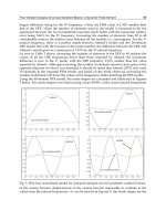
An instance of the coupled Rössler systems, with C = 0.5, is presented figure 4 as well as the
corresponding surrogates measure profile. We can clearly see that the original
synchronization value
H
xy
2
/
is above the imposed coupling value C. The relatively high
values of the measure obtained with the surrogates suggest that a non negligible amount of
the observed synchronization value is due to a linear component between the systems.


0 50 100 150 200 250 300 350 400
-40
-20
0
20
40
A.U.
Time (s)
0 100 200 300 400 500 600 700 800 900 1000
0
0.2
0.4
0.6

0.8
1
Surrogate number
Coupling


H
2
surr.
H
2
y/x

Fig. 4. Example of the output of the model for C = 0.5 (top panel) and surrogates measure
profile (bottom panel).

The distribution of the surrogate profile is depicted figure 5. We can easily see that the
distribution is highly non Gaussian and is best fitted by a Gamma law. A statistical test
based on the z-value might thus be erroneous. The non Gaussianity was attested by a
Lilliefors test applied on the experimental data. The 90 percentile derived from the fitted law
was 0.38. The measured coupling, 0.87 as observed figure 4, is above the 90 percentile and
thus attests of significant test. The proposed corrected measure,
H
cx
2
, is in this case 0.49
which is closer to the imposed coupling value C = 0.5 than the original measure.
0 0.1 0.2 0.3 0.4 0.5 0.6 0.7
0
0.5

1
1.5
2
2.5
3
3.5
4
4.5
5
Data
Density


H
2
surr.

(

,

)
N(

,

)

Fig. 5. Distribution of the surrogate values (Θ
0

), Gamma law model (Γ(α,β), continuous line)
and normal law model (N(μ,σ), dotted line).
Sources of bias in synchronization measures and how to minimize their effects on the
estimation of synchronicity: Application to the uterine electromyogram 83

and variance. The Lilliefors test is on the contrary based on a mean and variance of the
distribution derived directly from the data.

5.3 Percentile corrected statistic and associated hypothesis test
The distributions of Θ
0
might be non Gaussian as attested by a Lilliefors test for example. In
that case, the use of z-score statistics may be erroneous or at least meaningless. We propose
to use instead a measure corrected according to the statistics of the surrogates. This
measure, Θ
cx
, is defined as:
)(
01

xcx
P
(7)
where P
x
(y) stands for the x
th
percentile of the data y.
The study of the statistical distribution of Θ
0

allows us to define a statistical test even when
dealing with non Gaussian distributions. In practice, we have noticed that the distribution of
Θ
0
follows approximately a Gamma law Γ(α, β) when the distribution is not Gaussian. A
distribution model can be fitted directly on the surrogate data by maximum likelihood
estimation. This model allows us to easily define a statistical threshold for a given
probability p, over which the observed value Θ
1
is considered as significant. The inverse of
the Gamma cumulative distribution function, parameterized by the fitted α and β, gives the
threshold knowing the chosen probability p.
In the context of using the nonlinear correlation coefficient
2
H , we called the corrected
measure Θ
cx
,
H
cx
2
or surrogate corrected nonlinear correlation coefficient. This statistic is
bounded between [-1, 1] where the sign roughly indicates a non significant test if the
percentile x and the probability p coincide. According to the characteristics of the generated
surrogate data in this study, the parameter
H
cx
2
represents the part of the original
2

H value
unexplained by the linearity presents in the original time series.
From a practical point of view, the only parameter that has to be tuned is the number of
surrogates used to construct the surrogate measure profile. This number must be large
enough for a good estimation of the density function. It varies largely from one signal to
another. The counterparts of choosing a very high number of surrogates is the time of
computation especially with long original time series. After empirical evaluation of this
parameter, we found that 10000 surrogates was a good compromise for our signals.

5.4 Results on synthetic signals
For this experiment we used the following Rössler system configuration: ω
1
= 0.55 and ω
2
=
0.45. The sampling rate was 256 Hz.

An instance of the coupled Rössler systems, with C = 0.5, is presented figure 4 as well as the
corresponding surrogates measure profile. We can clearly see that the original
synchronization value
H
xy
2
/
is above the imposed coupling value C. The relatively high
values of the measure obtained with the surrogates suggest that a non negligible amount of
the observed synchronization value is due to a linear component between the systems.


0 50 100 150 200 250 300 350 400

-40
-20
0
20
40
A.U.
Time (s)
0 100 200 300 400 500 600 700 800 900 1000
0
0.2
0.4
0.6
0.8
1
Surrogate number
Coupling


H
2
surr.
H
2
y/x

Fig. 4. Example of the output of the model for C = 0.5 (top panel) and surrogates measure
profile (bottom panel).

The distribution of the surrogate profile is depicted figure 5. We can easily see that the
distribution is highly non Gaussian and is best fitted by a Gamma law. A statistical test

based on the z-value might thus be erroneous. The non Gaussianity was attested by a
Lilliefors test applied on the experimental data. The 90 percentile derived from the fitted law
was 0.38. The measured coupling, 0.87 as observed figure 4, is above the 90 percentile and
thus attests of significant test. The proposed corrected measure,
H
cx
2
, is in this case 0.49
which is closer to the imposed coupling value C = 0.5 than the original measure.
0 0.1 0.2 0.3 0.4 0.5 0.6 0.7
0
0.5
1
1.5
2
2.5
3
3.5
4
4.5
5
Data
Density


H
2
surr.

(


,

)
N(

,

)

Fig. 5. Distribution of the surrogate values (Θ
0
), Gamma law model (Γ(α,β), continuous line)
and normal law model (N(μ,σ), dotted line).
Recent Advances in Biomedical Engineering84

The original synchronization values were always above the imposed coupling (Figure 6).
For moderate couplings, below 0.5, the proposed correction gives nearly identical values as
the imposed coupling. From a coupling of 0.5, the proposed correction underestimates the
coupling strength between the systems. More importantly, we can notice that the difference
between the original and the corrected values is nearly constant. It indicates that the nature
of the relationship between the Rössler systems is identical whatever the imposed coupling
strength. This might explain the underestimation of the corrected synchronization due to a
“saturation” of the original synchronization at values near 1.
0.1 0.2 0.3 0.4 0.5 0.6 0.7 0.8 0.9
0
0.1
0.2
0.3
0.4

0.5
0.6
0.7
0.8
0.9
1
Imposed coupling
Measured Coupling


H
2
y/x
H
2
c90
ref.

Fig. 6. Original and corrected H
2
estimations (μ±σ) for different imposed coupling values.

5.5 Results on real EHG signals
Uterine EMG was recorded on a monkey during labor. Two bipolar channels were sutured
on the uterus approximately 7 cm apart. The two EMG channels were digitalized
simultaneously at 50 Hz. A detailed description of the experimental setup can be found in
(Terrien & al., 2008a). The EMG signals were then segmented manually to extract segments
containing uterine contractions. The different segments were then band-pass filtered (1 - 4.7
Hz) to extract FWH according to (Devedeux & al., 1983) by a 4
th

order phase preserving
Butterworth filter. We also showed that a time delay of EHG bursts highlight the synchrony
between the signals (Terrien & al., 2008b). The time delay between bursts that we chose
corresponds to the delay needed to maximize the cross-correlation function.

When applied to uterine EMG, we noticed very different behavior of H
2
in pregnancy and
labor contractions as depicted figure 7. In this example, even if the two contractions present
nearly the same original synchronization values (0.13 and 0.15), their surrogate measure
profiles are very different. For the labor contraction, the synchronization measures obtained
on surrogates are very low when compared to the original value contrary to the pregnancy
EMG, where some surrogates present synchronization measure above the original one. This

may indicate a strong relationship between the nonlinear components of the EMG burst
during labor which seems to be absent or less important during pregnancy. We consider
these differences to be useful in differentiating labor and pregnancy contractions.
Concerning the statistical test all labor contractions presented a significant test. For
pregnancy contractions, the majority but not all the contractions did not test as significant.

0 100 200 300 400 500 600 700 800 900 1000
0
0.05
0.1
0.15
0.2
Coupling
Labor contraction



0 100 200 300 400 500 600 700 800 900 1000
0
0.05
0.1
0.15
0.2
Surrogate number
Coupling
Pregnancy contraction


H
2
surr.
H
2
y/x
H
2
surr.
H
2
y/x

Fig. 7. Example of surrogates measure profile obtained with a labor contraction (top panel)
and a pregnancy contraction (bottom panel).

5.6 Discussion
Surrogates are constructed to fulfill all characteristics of a null hypothesis that we want to
evaluate on a time series. The statistical tests of the considered hypothesis use the z score

which implicitly assumes the Gaussianity of the surrogate statistic distribution. In case of non
Gaussian statistics, the usual test might fail or simply gives rise to erroneous conclusion. We
proposed to use, instead of the z-score, a percentile corrected statistic. This corrected value is
thought to be independent of the surrogate distribution. We derived a statistical test by simply
fitting the surrogate distribution by a given distribution model and defining a statistical
threshold. We demonstrated the satisfactory use of the proposed approach on synthetic and
real signals as well. When applied to the nonlinear correlation coefficient, we showed that the
statistics of the surrogate measure profile present a Gamma distribution, probably explained
by the quadratic nature of the original statistic. For this particular statistic, the new value
represents the part of the original value not explained by the linearity present in the original
time series. The usefulness of this new measure has of course to be confirmed and tested on
different type of data usually used in the field, EEG for example.
The use of this “new” synchronization measure on uterine EMG helped us to show two
different behaviors of contractions. We think that this difference might help us in
differentiating inefficient (pregnancy) and efficient (labor) contractions in the final aim of
labor prediction. This difference in behavior might be explained by the increase in the
nonlinearity of the EHG as labor approaches (Radhakrishnan & al., 2000). The surrogates
Sources of bias in synchronization measures and how to minimize their effects on the
estimation of synchronicity: Application to the uterine electromyogram 85

The original synchronization values were always above the imposed coupling (Figure 6).
For moderate couplings, below 0.5, the proposed correction gives nearly identical values as
the imposed coupling. From a coupling of 0.5, the proposed correction underestimates the
coupling strength between the systems. More importantly, we can notice that the difference
between the original and the corrected values is nearly constant. It indicates that the nature
of the relationship between the Rössler systems is identical whatever the imposed coupling
strength. This might explain the underestimation of the corrected synchronization due to a
“saturation” of the original synchronization at values near 1.
0.1 0.2 0.3 0.4 0.5 0.6 0.7 0.8 0.9
0

0.1
0.2
0.3
0.4
0.5
0.6
0.7
0.8
0.9
1
Imposed coupling
Measured Coupling


H
2
y/x
H
2
c90
ref.

Fig. 6. Original and corrected H
2
estimations (μ±σ) for different imposed coupling values.

5.5 Results on real EHG signals
Uterine EMG was recorded on a monkey during labor. Two bipolar channels were sutured
on the uterus approximately 7 cm apart. The two EMG channels were digitalized
simultaneously at 50 Hz. A detailed description of the experimental setup can be found in

(Terrien & al., 2008a). The EMG signals were then segmented manually to extract segments
containing uterine contractions. The different segments were then band-pass filtered (1 - 4.7
Hz) to extract FWH according to (Devedeux & al., 1983) by a 4
th
order phase preserving
Butterworth filter. We also showed that a time delay of EHG bursts highlight the synchrony
between the signals (Terrien & al., 2008b). The time delay between bursts that we chose
corresponds to the delay needed to maximize the cross-correlation function.

When applied to uterine EMG, we noticed very different behavior of H
2
in pregnancy and
labor contractions as depicted figure 7. In this example, even if the two contractions present
nearly the same original synchronization values (0.13 and 0.15), their surrogate measure
profiles are very different. For the labor contraction, the synchronization measures obtained
on surrogates are very low when compared to the original value contrary to the pregnancy
EMG, where some surrogates present synchronization measure above the original one. This

may indicate a strong relationship between the nonlinear components of the EMG burst
during labor which seems to be absent or less important during pregnancy. We consider
these differences to be useful in differentiating labor and pregnancy contractions.
Concerning the statistical test all labor contractions presented a significant test. For
pregnancy contractions, the majority but not all the contractions did not test as significant.

0 100 200 300 400 500 600 700 800 900 1000
0
0.05
0.1
0.15
0.2

Coupling
Labor contraction


0 100 200 300 400 500 600 700 800 900 1000
0
0.05
0.1
0.15
0.2
Surrogate number
Coupling
Pregnancy contraction


H
2
surr.
H
2
y/x
H
2
surr.
H
2
y/x

Fig. 7. Example of surrogates measure profile obtained with a labor contraction (top panel)
and a pregnancy contraction (bottom panel).


5.6 Discussion
Surrogates are constructed to fulfill all characteristics of a null hypothesis that we want to
evaluate on a time series. The statistical tests of the considered hypothesis use the z score
which implicitly assumes the Gaussianity of the surrogate statistic distribution. In case of non
Gaussian statistics, the usual test might fail or simply gives rise to erroneous conclusion. We
proposed to use, instead of the z-score, a percentile corrected statistic. This corrected value is
thought to be independent of the surrogate distribution. We derived a statistical test by simply
fitting the surrogate distribution by a given distribution model and defining a statistical
threshold. We demonstrated the satisfactory use of the proposed approach on synthetic and
real signals as well. When applied to the nonlinear correlation coefficient, we showed that the
statistics of the surrogate measure profile present a Gamma distribution, probably explained
by the quadratic nature of the original statistic. For this particular statistic, the new value
represents the part of the original value not explained by the linearity present in the original
time series. The usefulness of this new measure has of course to be confirmed and tested on
different type of data usually used in the field, EEG for example.
The use of this “new” synchronization measure on uterine EMG helped us to show two
different behaviors of contractions. We think that this difference might help us in
differentiating inefficient (pregnancy) and efficient (labor) contractions in the final aim of
labor prediction. This difference in behavior might be explained by the increase in the
nonlinearity of the EHG as labor approaches (Radhakrishnan & al., 2000). The surrogates
Recent Advances in Biomedical Engineering86

used in this study are also a stationarized version of the original time series. In the case of
uterine EMG, we assumed that the EMG bursts were stationary and we imputed the
difference between pregnancy and labor to a change in linearity only. Without testing this
stationary assumption, we could not be sure about the origin of the observed differences, i.e.
linearity or stationarity. The use of surrogates which preserve the non stationarity of the
original time series might be helpful for that purpose (Schreiber & Schmitz, 2000). As a first
way to answer this open question, we decided to study the influence of the non stationarity

in synchronization analysis and to propose an approach able to take into account this
information which is another source of bias of synchronization measure.

6. Dealing with non stationary signals
Most synchronization measures are only reliable in the analysis of long stationary time
series. A stationary signal is a signal which has all statistical moments constant with time.
This strong assumption might be relaxed since this property is impossible to verify. This
relaxed condition is called “weak stationarity“ of order n. A weak stationary signal of order
n presents all moments up to n that do not vary with time. The stationarity of order 2 is
often used (Blanco & al., 1995).
Many biological signals are however highly non stationary. Nevertheless, the coupling
analysis of these non stationary signals is usually performed by using a sliding window in
which the signals of interest are supposed to be stationary, or by directly using time
dependant synchronization measures like time-frequency approach (Ansary-Asl & al., 2006).
The most commonly used approach is the windowing method. The length of the window
has to be set according to the characteristics of the signal of interest. A bad choice of this
parameter might have dramatic effects on the obtained results. We propose to use instead a
pre-processing step able to detect automatically the longer stationary segments of a signal of
interest. This approach avoids making any trade off between the length of the segments and
the stationary assumption.

6.1 The windowing approach
The windowing approach consists in computing the synchronization parameter in a
window of finite length L, supposed to be the minimal stationary length of the signals of
interest, and shifting the window by a time τ before computing another value. The time shift
is often expressed as a percentage of overlapping between successive windows. The main
problem of this method is the estimation of the minimal stationary length.

A tradeoff between the length of the analysis window and the stationary assumption has to
be made. The length of the window also limits the accuracy of the time detection of abrupt

changes that can reflect biological mechanisms in the underlying systems. As it can be seen
figure 8, an increase in the length of the analysis window reduces the variance of the
estimation but at a same time smoothes the boundary of the transition times, located in this
example roughly at 204 and 460 s. The length of the window is thus an important parameter
which has to be set according to a prior knowledge of the minimal length of the stationary
parts of the signals or by trial and error.

0 100 200 300 400 500 600 700 800 900
-40
-20
0
20
40
A.U.
0 100 200 300 400 500 600 700 800 900
0
0.2
0.4
0.6
0.8
1
Time (s)
Coupling


Ref.
40 s
20 s

Fig. 8. Example of the output of the Rössler system (top panel) and the corresponding

synchronization analysis using H
2
(bottom panel) obtained by the windowing approach for
a window length of 40 s or 20 s. The coupling function C(t) is presented as a continuous line
(Ref.).

6.2 Piecewise stationary pre-segmentation (PSP) approach
Piecewise stationary segmentation algorithms are designed to detect all local stationary
partitions composing a signal of interest. They are different from event segmentation
algorithms which are designed to detect events of interest, stationary or not, inside a signal.
They are mostly based on the analysis of the local statistical properties of the signal. In the
context of synchronization analysis, we used advantageously one of these algorithms in
order to detect the longer stationary parts inside the signals of interest before applying the
traditional synchronization measure. Its results in a succession of windows of automatically
locally adapted length. We call this pre-processing step: Piecewise stationary pre-
segmentation or PSP.

The PSP algorithm has been proven to be useful as pre-treatment of synchronization
analysis (Terrien & al., 2008b). In the case of different stationarity changes in the two
channels, the univariate PSP (uPSP) method, described in (Terrien & al., 2008b), might fail to
detect these changes. It is explained by the nature of this algorithm which only uses one of
both channels for the segmentation. In order to be able to deal properly with this situation,
we slightly modified the uPSP algorithm. Instead of using the auto spectrum of only one
channel, the stationarity changes are detected using the cross spectrum, thus taking into
account the statistical changes in both channels at the same time. We called this method
bivariate PSP or bPSP for short. This algorithm, also based on the algorithm developed by
Carré and Fernandez (Carré & Fernandez, 1998), can be described briefly as follows:

Sources of bias in synchronization measures and how to minimize their effects on the
estimation of synchronicity: Application to the uterine electromyogram 87


used in this study are also a stationarized version of the original time series. In the case of
uterine EMG, we assumed that the EMG bursts were stationary and we imputed the
difference between pregnancy and labor to a change in linearity only. Without testing this
stationary assumption, we could not be sure about the origin of the observed differences, i.e.
linearity or stationarity. The use of surrogates which preserve the non stationarity of the
original time series might be helpful for that purpose (Schreiber & Schmitz, 2000). As a first
way to answer this open question, we decided to study the influence of the non stationarity
in synchronization analysis and to propose an approach able to take into account this
information which is another source of bias of synchronization measure.

6. Dealing with non stationary signals
Most synchronization measures are only reliable in the analysis of long stationary time
series. A stationary signal is a signal which has all statistical moments constant with time.
This strong assumption might be relaxed since this property is impossible to verify. This
relaxed condition is called “weak stationarity“ of order n. A weak stationary signal of order
n presents all moments up to n that do not vary with time. The stationarity of order 2 is
often used (Blanco & al., 1995).
Many biological signals are however highly non stationary. Nevertheless, the coupling
analysis of these non stationary signals is usually performed by using a sliding window in
which the signals of interest are supposed to be stationary, or by directly using time
dependant synchronization measures like time-frequency approach (Ansary-Asl & al., 2006).
The most commonly used approach is the windowing method. The length of the window
has to be set according to the characteristics of the signal of interest. A bad choice of this
parameter might have dramatic effects on the obtained results. We propose to use instead a
pre-processing step able to detect automatically the longer stationary segments of a signal of
interest. This approach avoids making any trade off between the length of the segments and
the stationary assumption.

6.1 The windowing approach

The windowing approach consists in computing the synchronization parameter in a
window of finite length L, supposed to be the minimal stationary length of the signals of
interest, and shifting the window by a time τ before computing another value. The time shift
is often expressed as a percentage of overlapping between successive windows. The main
problem of this method is the estimation of the minimal stationary length.

A tradeoff between the length of the analysis window and the stationary assumption has to
be made. The length of the window also limits the accuracy of the time detection of abrupt
changes that can reflect biological mechanisms in the underlying systems. As it can be seen
figure 8, an increase in the length of the analysis window reduces the variance of the
estimation but at a same time smoothes the boundary of the transition times, located in this
example roughly at 204 and 460 s. The length of the window is thus an important parameter
which has to be set according to a prior knowledge of the minimal length of the stationary
parts of the signals or by trial and error.

0 100 200 300 400 500 600 700 800 900
-40
-20
0
20
40
A.U.
0 100 200 300 400 500 600 700 800 900
0
0.2
0.4
0.6
0.8
1
Time (s)

Coupling


Ref.
40 s
20 s

Fig. 8. Example of the output of the Rössler system (top panel) and the corresponding
synchronization analysis using H
2
(bottom panel) obtained by the windowing approach for
a window length of 40 s or 20 s. The coupling function C(t) is presented as a continuous line
(Ref.).

6.2 Piecewise stationary pre-segmentation (PSP) approach
Piecewise stationary segmentation algorithms are designed to detect all local stationary
partitions composing a signal of interest. They are different from event segmentation
algorithms which are designed to detect events of interest, stationary or not, inside a signal.
They are mostly based on the analysis of the local statistical properties of the signal. In the
context of synchronization analysis, we used advantageously one of these algorithms in
order to detect the longer stationary parts inside the signals of interest before applying the
traditional synchronization measure. Its results in a succession of windows of automatically
locally adapted length. We call this pre-processing step: Piecewise stationary pre-
segmentation or PSP.

The PSP algorithm has been proven to be useful as pre-treatment of synchronization
analysis (Terrien & al., 2008b). In the case of different stationarity changes in the two
channels, the univariate PSP (uPSP) method, described in (Terrien & al., 2008b), might fail to
detect these changes. It is explained by the nature of this algorithm which only uses one of
both channels for the segmentation. In order to be able to deal properly with this situation,

we slightly modified the uPSP algorithm. Instead of using the auto spectrum of only one
channel, the stationarity changes are detected using the cross spectrum, thus taking into
account the statistical changes in both channels at the same time. We called this method
bivariate PSP or bPSP for short. This algorithm, also based on the algorithm developed by
Carré and Fernandez (Carré & Fernandez, 1998), can be described briefly as follows:

Recent Advances in Biomedical Engineering88

1. Decompose the signal x and y into successive dyadic partitions up to chosen
decomposition level L+1
2. Compute and denoise, by undecimated wavelet transform, the log cross spectrum of
each partition
3. Compute a binary tree of spectral distances between adjacent partitions
4. Search for the tree which minimizes the sum of the spectral distances by a modified
version of the best basis algorithm of Coifman Wickerhauser
5. Apply the post processing steps described in (Carré & Fernandez, 1998) to deal
properly with non dyadic partitions
The post processing steps consist mainly in applying the step 1 to 4 on each non terminal
node with one level of decomposition and using the original best basis algorithm.
Our modified version of the best basis algorithm differs from the original one only by the
node selection rule. This modification was necessary to differentiate the increase in the
spectral distances due to the bias of the estimator, or due to signal symmetry around the
considered cutting point. Each node n
i,j
has a cost, corresponding to the spectral distance, c
i,j
.
The classical decision rule concerning the selection of a father node c
i,j
is:

if (c
i,j
≤ c
i+1,2j
+ c
i+1,2j+1
) then
Mark the node as a part of the best basis
else
c
i,j
= c
i+1,2j
+ c
i+1,2j+1

endif
The empirical modification of the selection rule is simply α.c
i,j
≤ c
i+1,2j
+ c
i+1,2j+1
with α > 2. We
chose α = 2.5.
We showed that the use of the bPSP method avoids an arbitrary choice of the channel to
which the stationary segmentation is based on and takes in to account the non stationarity of
both signals present.
In a practical point of view, the parameters used in this method are mainly the number of
decomposition levels in the segmentation procedure and in the wavelet denoising. These

parameters are independent. The first one controls the minimal stationary length that the
algorithm can detect. It must be roughly adapted to the signal of interest. A too high number
of levels might increase the spectral estimation error, and lead to bad segmentation, due to
an increased bias of the cross periodogram. The second parameter controlling the denoising
of the spectra might lead to over smoothing of the estimated spectra and thus miss some
important features in the different local stationary zones.

6.3 Results on synthetic signals
The configuration of the Rössler system used in this study is summarized table 2. The
sampling rate used was 10 Hz.

Time t (s) ω
1
(t)

ω
2
(t)

C(t)
0 - 204.8 0.65 0.55 0.3
204.8 - 307.2

1.2 0.55 0.01

307.2 - 460.8

1.2 1.1 0.8
460.8 - 563.3


0.65 1.1 0.01

563.3 - 819.1

0.65 0.5 0.5
Table 2. Parameters of the coupled Rössler system.

Figure 9 presents one example of the synthetic signals used and the corresponding
synchronization analyses with H
2
. The results obtained by the windowing approach show a
synchronization pattern that approximately follows the coupling function. Important
differences can be found during periods of low coupling between the two signals. Increasing
the length of the window allowed us to significantly decrease the amplitude of the
variations of the parameter but at the same time the boundaries of the different coupling
periods become smoother. The bPSP approach shows marked transitions between the
different coupling periods with relatively constant parameter values. More importantly, the
algorithm is able to detect the change points situated at 307.2 and 563.3 s. This time instant
corresponds to changes occurring in the second signals. The previous algorithm, presented
in (Terrien & al., 2008b), would not have detected this transition, when using the top signal
as reference, and not the transitions at 205 and 470 seconds when using the lower signal as
reference. The differences between the coupling function C(t) and the estimates are due to
the intrinsic bias of H
2
as already highlighted in figure 6 of the paragraph 5.
0 100 200 300 400 500 600 700 800
-40
-20
0
20

40
A.U.
0 100 200 300 400 500 600 700 800
0
0.2
0.4
0.6
0.8
1
Time (s)
Coupling


1
2
3

Fig. 9. Example of the output of the Rössler system (top panel) and the corresponding
synchronization analysis using H
2
(bottom panel) obtained by the bPSP (2) and the
windowing approach for a window length of 40 s (3). The coupling function C(t) is
presented as a continuous line (1).

We might be interested in the robustness of a particular method or algorithm in order to
apprehend its behavior in the presence of noise. This step is important since most biological
signals are very noisy. The main parameters used in robustness analysis are the bias and the
variance of the estimator.
We evaluated the robustness of the segmentation algorithm by Monte-Carlo simulations.
For different noise (Gaussian white noise) levels, as express by the SNR, the bias and

variance of the estimators were computed against the parameter values computed in the
reference segments (segments that we would have obtained with a perfect segmentation).
Sources of bias in synchronization measures and how to minimize their effects on the
estimation of synchronicity: Application to the uterine electromyogram 89

1. Decompose the signal x and y into successive dyadic partitions up to chosen
decomposition level L+1
2. Compute and denoise, by undecimated wavelet transform, the log cross spectrum of
each partition
3. Compute a binary tree of spectral distances between adjacent partitions
4. Search for the tree which minimizes the sum of the spectral distances by a modified
version of the best basis algorithm of Coifman Wickerhauser
5. Apply the post processing steps described in (Carré & Fernandez, 1998) to deal
properly with non dyadic partitions
The post processing steps consist mainly in applying the step 1 to 4 on each non terminal
node with one level of decomposition and using the original best basis algorithm.
Our modified version of the best basis algorithm differs from the original one only by the
node selection rule. This modification was necessary to differentiate the increase in the
spectral distances due to the bias of the estimator, or due to signal symmetry around the
considered cutting point. Each node n
i,j
has a cost, corresponding to the spectral distance, c
i,j
.
The classical decision rule concerning the selection of a father node c
i,j
is:
if (c
i,j
≤ c

i+1,2j
+ c
i+1,2j+1
) then
Mark the node as a part of the best basis
else
c
i,j
= c
i+1,2j
+ c
i+1,2j+1

endif
The empirical modification of the selection rule is simply α.c
i,j
≤ c
i+1,2j
+ c
i+1,2j+1
with α > 2. We
chose α = 2.5.
We showed that the use of the bPSP method avoids an arbitrary choice of the channel to
which the stationary segmentation is based on and takes in to account the non stationarity of
both signals present.
In a practical point of view, the parameters used in this method are mainly the number of
decomposition levels in the segmentation procedure and in the wavelet denoising. These
parameters are independent. The first one controls the minimal stationary length that the
algorithm can detect. It must be roughly adapted to the signal of interest. A too high number
of levels might increase the spectral estimation error, and lead to bad segmentation, due to

an increased bias of the cross periodogram. The second parameter controlling the denoising
of the spectra might lead to over smoothing of the estimated spectra and thus miss some
important features in the different local stationary zones.

6.3 Results on synthetic signals
The configuration of the Rössler system used in this study is summarized table 2. The
sampling rate used was 10 Hz.

Time t (s) ω
1
(t)

ω
2
(t)

C(t)
0 - 204.8 0.65 0.55 0.3
204.8 - 307.2

1.2 0.55 0.01

307.2 - 460.8

1.2 1.1 0.8
460.8 - 563.3

0.65 1.1 0.01

563.3 - 819.1


0.65 0.5 0.5
Table 2. Parameters of the coupled Rössler system.

Figure 9 presents one example of the synthetic signals used and the corresponding
synchronization analyses with H
2
. The results obtained by the windowing approach show a
synchronization pattern that approximately follows the coupling function. Important
differences can be found during periods of low coupling between the two signals. Increasing
the length of the window allowed us to significantly decrease the amplitude of the
variations of the parameter but at the same time the boundaries of the different coupling
periods become smoother. The bPSP approach shows marked transitions between the
different coupling periods with relatively constant parameter values. More importantly, the
algorithm is able to detect the change points situated at 307.2 and 563.3 s. This time instant
corresponds to changes occurring in the second signals. The previous algorithm, presented
in (Terrien & al., 2008b), would not have detected this transition, when using the top signal
as reference, and not the transitions at 205 and 470 seconds when using the lower signal as
reference. The differences between the coupling function C(t) and the estimates are due to
the intrinsic bias of H
2
as already highlighted in figure 6 of the paragraph 5.
0 100 200 300 400 500 600 700 800
-40
-20
0
20
40
A.U.
0 100 200 300 400 500 600 700 800

0
0.2
0.4
0.6
0.8
1
Time (s)
Coupling


1
2
3

Fig. 9. Example of the output of the Rössler system (top panel) and the corresponding
synchronization analysis using H
2
(bottom panel) obtained by the bPSP (2) and the
windowing approach for a window length of 40 s (3). The coupling function C(t) is
presented as a continuous line (1).

We might be interested in the robustness of a particular method or algorithm in order to
apprehend its behavior in the presence of noise. This step is important since most biological
signals are very noisy. The main parameters used in robustness analysis are the bias and the
variance of the estimator.
We evaluated the robustness of the segmentation algorithm by Monte-Carlo simulations.
For different noise (Gaussian white noise) levels, as express by the SNR, the bias and
variance of the estimators were computed against the parameter values computed in the
reference segments (segments that we would have obtained with a perfect segmentation).
Recent Advances in Biomedical Engineering90


This methodology allowed us to take into account the intrinsic bias of the synchronization
measure.
The robustness analysis (bias and variance) for the parameters H
2
is presented figure 10. The
stationary approach presents a lower bias than the windowing approach whatever the noise
level. The variance obtained by the bPSP method is however greater. The analysis of the
individual results showed that this high variance is mainly due to an over segmentation of
each stationary zone.
Inf 30 20 10 0
0
0.02
0.04
0.06
0.08
0.1
|Bias H
2
|


Stationary
Window
Inf 30 20 10 0
0
1
2
x 10
-4

SNR (dB)
Variance H
2


Stationary
Window

Fig. 10. Absolute value of the bias (top panel) and variance (bottom panel) obtained with the
bPSP (continuous line) and the windowing approach (dotted line) for the parameter H
2
.

6.4 Results on real EHG signals
The results of the segmentation of a broad band and narrow band contractile event recorded
during labor are presented figure 11. We can clearly see, on both types of signals, that the
algorithm is able to take into account changes occurring in both channels.


0 5 10 15 20 25 30 35 40 45
-500
0
500

V
Broad band signal
0 5 10 15 20 25 30 35 40 45
-500
0
500

Time (s)

V
Narrow band signal

Fig. 11. Example of an electrical contraction burst recorded during the same contraction
occurring in labor and their segmentation considering the broad band signals, raw signals
(top panel), or a narrow band version of them, FWH filtered (bottom panel).

The results obtained with H
2
are presented figure 12. On the non shifted broad band signal
the values of H
2
observed inside the contractile event are similar to those observed during
the base lines (non EMG segments present before 10 s and after 35 s). The time shift of the
signal of the second channel to compensate for the propagation delay of the contraction does
not change the parameter pattern significantly. Only the first base line presents lower
synchronization values as compared with no time shift. With the narrow band version of the
signals, an increase in the parameter H
2
is clearly observable inside the contractile event
when compared to the base line segments. The base lines still present relatively high values.
The time shift of 0.18 s of the second signal causes a strong decrease in the base line values,
while the values inside the contractile event increase or stay high. The effects of the time
shift is less clear on the narrow band signal maybe due to the short delay between the two
channels.
Looking at the results obtained with the windowing approach, no specific pattern can be
observed in the same conditions. Moreover, the base lines present stronger or similar values
of synchronicity than inside the contractions whatever the considered situation. Similar

results were obtained for the other contractions tested.

Sources of bias in synchronization measures and how to minimize their effects on the
estimation of synchronicity: Application to the uterine electromyogram 91

This methodology allowed us to take into account the intrinsic bias of the synchronization
measure.
The robustness analysis (bias and variance) for the parameters H
2
is presented figure 10. The
stationary approach presents a lower bias than the windowing approach whatever the noise
level. The variance obtained by the bPSP method is however greater. The analysis of the
individual results showed that this high variance is mainly due to an over segmentation of
each stationary zone.
Inf 30 20 10 0
0
0.02
0.04
0.06
0.08
0.1
|Bias H
2
|


Stationary
Window
Inf 30 20 10 0
0

1
2
x 10
-4
SNR (dB)
Variance H
2


Stationary
Window

Fig. 10. Absolute value of the bias (top panel) and variance (bottom panel) obtained with the
bPSP (continuous line) and the windowing approach (dotted line) for the parameter H
2
.

6.4 Results on real EHG signals
The results of the segmentation of a broad band and narrow band contractile event recorded
during labor are presented figure 11. We can clearly see, on both types of signals, that the
algorithm is able to take into account changes occurring in both channels.


0 5 10 15 20 25 30 35 40 45
-500
0
500

V
Broad band signal

0 5 10 15 20 25 30 35 40 45
-500
0
500
Time (s)

V
Narrow band signal

Fig. 11. Example of an electrical contraction burst recorded during the same contraction
occurring in labor and their segmentation considering the broad band signals, raw signals
(top panel), or a narrow band version of them, FWH filtered (bottom panel).

The results obtained with H
2
are presented figure 12. On the non shifted broad band signal
the values of H
2
observed inside the contractile event are similar to those observed during
the base lines (non EMG segments present before 10 s and after 35 s). The time shift of the
signal of the second channel to compensate for the propagation delay of the contraction does
not change the parameter pattern significantly. Only the first base line presents lower
synchronization values as compared with no time shift. With the narrow band version of the
signals, an increase in the parameter H
2
is clearly observable inside the contractile event
when compared to the base line segments. The base lines still present relatively high values.
The time shift of 0.18 s of the second signal causes a strong decrease in the base line values,
while the values inside the contractile event increase or stay high. The effects of the time
shift is less clear on the narrow band signal maybe due to the short delay between the two

channels.
Looking at the results obtained with the windowing approach, no specific pattern can be
observed in the same conditions. Moreover, the base lines present stronger or similar values
of synchronicity than inside the contractions whatever the considered situation. Similar
results were obtained for the other contractions tested.

Recent Advances in Biomedical Engineering92

0 10 20 30 40
0
0.2
0.4
0.6
0.8
1
Broad band EHG

= 0 s
0 10 20 30 40
0
0.2
0.4
0.6
0.8
1

= 0.18 s
0 10 20 30 40
0
0.1

0.2
0.3
0.4
0.5
Time (s)
Narrow band EHG
0 10 20 30 40
0
0.1
0.2
0.3
0.4
0.5
Time (s)

Fig. 12. H
2
profile obtained on the broad band (first line) or the narrow band (second line)
signal of the contractile event presented figure 11 and for no time shift (first column) or a
time shift of τ = 0.18 s (second column). The results obtained with the windowing approach
in the same conditions are plotted with dashed lines.

6.5 Discussion
Most physiological signals are non stationary. Their characterization is therefore often
difficult. In the context of synchronization analysis, the most commonly used approach is
the windowing of the signals of interest before computing the different synchronization
measures. The length of the analysis window is however an important parameter and
controls the trade-off between stationary assumption of the signals in the window and the
accuracy of the analysis. This parameter is often chosen as constant in time. We presented
the advantages of using an automatic segmentation procedure of the signal that search for

the longer locally adapted stationary parts in the context of synchronization analysis.
The bPSP approach shows reduced bias of the estimators when compared to the reference
segmentation. The obtained variance is however higher than with the windowing approach
due to over segmentation of the different stationary parts. A better control of the partition
fusion procedure in the algorithm might allow us to reduce this over segmentation. The
fusion procedure is based on a modification of the Coifman Wickerhauser algorithm,
controlled by the parameter α. The adaptation of this parameter to the signal of interest
might reduce this problem. The length of the minimal stationary zone is dependant of the
levels of decomposition. Even if this parameter can be adapted to the signal of interest, a too
high number of decomposition levels increases the bias of the spectral estimation due to the
shortness of the analyzed data segments. This can introduce errors in the detection of the
stationary parts of the signals. The use of other algorithms, which perform segmentation in a
continuous time, can be a solution if precise time detection is needed. We have shown that

the PSP method can be applied to signals with different characteristics and that it gives
satisfactory results when compared to the ones obtained with the windowing approach.
Specifically for real EHG, the numerous segments found on each analyzed burst confirm the
high non stationarity of the EHG signal, even when band-pass filtered. This might indicate
that the difference of surrogate measure profile characteristics between contractions is due
to a difference in non stationarity rather than of nonlinearity, even if we cannot exclude
definitively or totally this latter hypothesis. Both influences might coexist and be
independent. More investigations are thus necessary in order to obtain a clear answer.
We have shown that the use of this method can clearly identify the proper treatment,
filtering or time shift for example, needed to identify and highlight synchronization between
different parts of the uterus during labor. It might be of use to monitor the evolution of the
synchronization of the uterus from pregnancy to labor. This approach can also be used in
the determination of the optimal synchronization measure for the uterine EMG.

7. Labor prediction
7.1 ROC curve analysis

In order to evaluate the possible use of the proposed parameters for the prediction of labor
in monkey, we used the classical Receiver Operating Characteristic (ROC) curves. A ROC
curve is a graphical tool permitting to evaluate a binary, i.e. two classes, classifier. A ROC
curve is the curve corresponding to TPR (True Positive Rate or sensitivity) vs. FPR (False
Positive Rate or 1 - Specificity) obtained for different parameter thresholds. ROC curves are
classically compared by mean of the Area Under the Curve (AUC) and accuracy (ACC). The
AUC was estimated by the trapezoidal integration method. We additionally used the
Matthew’s Correlation Coefficient (MCC) defined as:
)()()()(
**
FPTPFNTPFPTNFNTN
FNFPTNTP
MCC




(8)
where TP, TN, FP and FN stand respectively for True Positive, True Negative, False Positve
and False Negative values.

7.2 Prediction using proposed corrected parameters
Under the hypothesis that the uterus synchronizes as labor approaches, we evaluated the
potential of the nonlinear correlation coefficient as a predictor of labor on monkey. We
evaluated the performance of the proposed parameters for labor prediction on a data set
containing 35 pregnancy and 34 labor contractions. We compared the predictive capability
of the nonlinear correlation coefficient (H
2
) and of the 90 percentile corrected nonlinear
correlation coefficient,

H
c
2
90
. We have shown that the segmentation into piecewise
stationary parts of EHG highlights synchronicity inside EHG burst, but gives rise to
multiple values of H
2
within one burst (one for each stationary segment). For comparison
purpose, we thus decided to also include the integral of the H
2
profile during the
bursts,

2
H
, as a synchronization parameter for labor prediction.
The average results obtained on our data set with the parameter
H
c
2
90
and H
2
are presented
table 3. We can see that the original values of H
2
are very similar or slightly lower during
Sources of bias in synchronization measures and how to minimize their effects on the
estimation of synchronicity: Application to the uterine electromyogram 93


0 10 20 30 40
0
0.2
0.4
0.6
0.8
1
Broad band EHG

= 0 s
0 10 20 30 40
0
0.2
0.4
0.6
0.8
1

= 0.18 s
0 10 20 30 40
0
0.1
0.2
0.3
0.4
0.5
Time (s)
Narrow band EHG
0 10 20 30 40

0
0.1
0.2
0.3
0.4
0.5
Time (s)

Fig. 12. H
2
profile obtained on the broad band (first line) or the narrow band (second line)
signal of the contractile event presented figure 11 and for no time shift (first column) or a
time shift of τ = 0.18 s (second column). The results obtained with the windowing approach
in the same conditions are plotted with dashed lines.

6.5 Discussion
Most physiological signals are non stationary. Their characterization is therefore often
difficult. In the context of synchronization analysis, the most commonly used approach is
the windowing of the signals of interest before computing the different synchronization
measures. The length of the analysis window is however an important parameter and
controls the trade-off between stationary assumption of the signals in the window and the
accuracy of the analysis. This parameter is often chosen as constant in time. We presented
the advantages of using an automatic segmentation procedure of the signal that search for
the longer locally adapted stationary parts in the context of synchronization analysis.
The bPSP approach shows reduced bias of the estimators when compared to the reference
segmentation. The obtained variance is however higher than with the windowing approach
due to over segmentation of the different stationary parts. A better control of the partition
fusion procedure in the algorithm might allow us to reduce this over segmentation. The
fusion procedure is based on a modification of the Coifman Wickerhauser algorithm,
controlled by the parameter α. The adaptation of this parameter to the signal of interest

might reduce this problem. The length of the minimal stationary zone is dependant of the
levels of decomposition. Even if this parameter can be adapted to the signal of interest, a too
high number of decomposition levels increases the bias of the spectral estimation due to the
shortness of the analyzed data segments. This can introduce errors in the detection of the
stationary parts of the signals. The use of other algorithms, which perform segmentation in a
continuous time, can be a solution if precise time detection is needed. We have shown that

the PSP method can be applied to signals with different characteristics and that it gives
satisfactory results when compared to the ones obtained with the windowing approach.
Specifically for real EHG, the numerous segments found on each analyzed burst confirm the
high non stationarity of the EHG signal, even when band-pass filtered. This might indicate
that the difference of surrogate measure profile characteristics between contractions is due
to a difference in non stationarity rather than of nonlinearity, even if we cannot exclude
definitively or totally this latter hypothesis. Both influences might coexist and be
independent. More investigations are thus necessary in order to obtain a clear answer.
We have shown that the use of this method can clearly identify the proper treatment,
filtering or time shift for example, needed to identify and highlight synchronization between
different parts of the uterus during labor. It might be of use to monitor the evolution of the
synchronization of the uterus from pregnancy to labor. This approach can also be used in
the determination of the optimal synchronization measure for the uterine EMG.

7. Labor prediction
7.1 ROC curve analysis
In order to evaluate the possible use of the proposed parameters for the prediction of labor
in monkey, we used the classical Receiver Operating Characteristic (ROC) curves. A ROC
curve is a graphical tool permitting to evaluate a binary, i.e. two classes, classifier. A ROC
curve is the curve corresponding to TPR (True Positive Rate or sensitivity) vs. FPR (False
Positive Rate or 1 - Specificity) obtained for different parameter thresholds. ROC curves are
classically compared by mean of the Area Under the Curve (AUC) and accuracy (ACC). The
AUC was estimated by the trapezoidal integration method. We additionally used the

Matthew’s Correlation Coefficient (MCC) defined as:
)()()()(
**
FPTPFNTPFPTNFNTN
FNFPTNTP
MCC




(8)
where TP, TN, FP and FN stand respectively for True Positive, True Negative, False Positve
and False Negative values.

7.2 Prediction using proposed corrected parameters
Under the hypothesis that the uterus synchronizes as labor approaches, we evaluated the
potential of the nonlinear correlation coefficient as a predictor of labor on monkey. We
evaluated the performance of the proposed parameters for labor prediction on a data set
containing 35 pregnancy and 34 labor contractions. We compared the predictive capability
of the nonlinear correlation coefficient (H
2
) and of the 90 percentile corrected nonlinear
correlation coefficient,
H
c
2
90
. We have shown that the segmentation into piecewise
stationary parts of EHG highlights synchronicity inside EHG burst, but gives rise to
multiple values of H

2
within one burst (one for each stationary segment). For comparison
purpose, we thus decided to also include the integral of the H
2
profile during the
bursts,

2
H
, as a synchronization parameter for labor prediction.
The average results obtained on our data set with the parameter
H
c
2
90
and H
2
are presented
table 3. We can see that the original values of H
2
are very similar or slightly lower during