Hindawi Publishing Corporation
EURASIP Journal on Advances in Signal Processing
Volume 2010, Article ID 690218, 11 pages
doi:10.1155/2010/690218
Research Article
A New Switching-Based Median Filtering Scheme and Algorithm
for Removal of High-Density Salt and Pepper Noise in Images
V. Jayaraj and D. Ebenezer
Dig ital Signal Processing Laboratory, Sri Krishna College of Engineering and Technology, Coimbatore,
Anna University Coimbatore, Tamilnadu 641008, India
Correspondence should be addressed to V. Jayaraj, jayaraj

Received 21 December 2009; Revised 8 May 2010; Accepted 17 June 2010
Academic Editor: Satya Dharanipragada
Copyright © 2010 V. Jayaraj and D. Ebenezer. This is an open access article distributed under the Creative Commons Attribution
License, which permits unrestricted use, distribution, and reproduction in any medium, provided the original work is properly
cited.
A new switching-based median filtering scheme for restoration of images that are highly corrupted by salt and pepper noise is
proposed. An algorithm based on the scheme is developed. The new scheme introduces the concept of substitution of noisy pixels
by linear prediction prior to estimation. A novel simplified linear predictor is developed for this purpose. The objective of the
scheme and algorithm is the removal of high-density salt and pepper noise in images. The new algorithm shows significantly
better image quality with good PSNR, reduced MSE, good edge preservation, and reduced streaking. The good performance is
achieved with reduced computational complexity. A comparison of the performance is made with several existing algorithms in
terms of visual and quantitative results. The performance of the proposed scheme and algorithm is demonstrated.
1. Introduction
Images are often corrupted by impulsive noise in addition
to several other types of noise. There are two models of
impulsive noise, namely, salt, and pepper noise and random
valued impulse noise. Salt and pepper noise is sometimes
called fixed valued impulse noise producing two gray level
values 0 and 255. Random valued impulse noise will produce

impulses whose gray level value lies within a predetermined
range. For example, if gray level exceeds a value L
Max
,itisa
positive impulse (L
Max
to 255); if gray level is less than L
Min
,
it is a negative impulse (0 to L
Min
). Impulse noise is caused by
faulty camera sensors, faults in data acquisition systems, and
transmission in a noisy channel. Median filtering has been
established as a reliable method to remove impulse noise
without damaging edge details [1, 2]. The Standard Median
Filter (SMF) is effective only at low noise densities. Several
methods have been proposed for removal of impulse noise at
higher noise densities [3–5]. Recently, computational com-
plexity has become an important consideration in impulse
noise removal. Use of a small size fixed window in median
filtering keeps the computational load a minimum. However,
small window size leads to insufficient noise reduction.
Switching-based median filtering has been proposed as an
effective alternative for reducing computational complexity.
This method involves detection of noisy pixels prior to
processing, and filtering is applied only to corrupted pixels
while leaving uncorrupted pixels intact. Several switching-
based methods have been proposed [6–21]. A recent method
named Decision Based Algorithm (DBA) is one of the fastest

methods and it is an efficient algorithm capable of impulse
noise removal at noise densities as high as 80% [16, 17]. A
major drawback of this algorithm is streaking at higher noise
densities. The median filter not only smoothes the noise in
homogeneous regions but it also tends to produce regions
of constant or nearly constant intensity. The shape of these
regions depends on the geometry of the filter window. They
are usually streaks (linear patches) or amorphous blotches.
Thesesideeffects of the median filter are highly undesirable,
because they are perceived as either lines or contours that
do not exist in the original image. The probability that two
successive outputs of the median filter y
i
, y
i+1
have the same
value is quite high
Pr

y
i
= y
i+1

= 0.5

1 −

1
n


(1)
2 EURASIP Journal on Advances in Signal Processing
when the input x
i
is a stationary r andom process. When
the window size “n” tends to infinity, this probability tends
to 0.5. Streaking and blotching are undesirable effects.
Postprocessing of the median filter output is desirable.
A better solution is to use other nonlinear filters based
on order statistics, which have better performance than
median filter with reduced streaking and computational
complexity. Streaking cannot b e neglected particularly in
high-density noise situations where a large number of pixels
in a processing window are noisy pixels. One strategy, which
is the simplest, is to replace the corrupted pixel by an
immediate uncorrupted pixel. When window is moved to
the next position, a similar situation arises. The replacement
involves repetition of the uncorrupted pixel. This repetition
causes streaking. In several algorithms such as adaptive
algorithms and robust estimation algorithms, this repetition
is less frequent and therefore is not as visible as in case of
DBA. This paper introduces a new switching-based median
filtering scheme and algorithm for removal of impulse noise
with reduced streaking under the constraint of reduced
computational complexity. The algorithm is also expected to
provide good noise performance and edge preservation. This
paper considers salt and pepper type impulse noise [12–17].
2. Switching-Based Median Filters
Switching-based median filters are well known. Identifying

noisy pixels and processing only noisy pixels is the main
principle in switching-based median filters. There are three
stages in switching-based median filtering, namely, noise
detection, estimation of noise-free pixels and replacement.
The principle of identifying noisy pixels and processing only
noisy pixels has been effective in reducing processing time
as well as image degradation. The limitation of sw itching
median filter is that defining a robust decision measure is
difficult because the decision is usually based on a predefined
threshold value. In addition the noisy pixels are replaced
by some median value in their vicinity without taking into
account local features such as presence of edges. Hence, edges
and fine details are not recovered satisfactorily, especial ly
when the noise level is high. In order to overcome these
drawbacks. Chan et al. [16] have proposed a two-phase
algorithm. In the first phase an adaptive median filter is used
to classify corrupted and uncorrupted pixels. In the second
phase, specialized regularization method is applied to the
noisy pixels to preserve the edges besides noise suppression.
The main drawback of this method is that the processing
time is very high because it uses very large window size.
There are several strategies for identification, processing,
and replacement of noisy pixels. The simplest strategy is
to replace the noisy pixels by the immediate neighborhood
pixel. The DBA [17] employs this strategy wherein the
computation time is the lowest among several standard
algorithms even at higher noise densities. A disadvantage
of this strategy is increased streaking. It is highly desirable
to limit streaking which degrades the final processed image.
This is indeed a challenging task under the constraint that the

processing time be kept as low as possible while preserving
edges and removing most of the noise.
3. New Switching-Based Median
Filtering Scheme
This paper de velops a new switching-based median filtering
scheme for tackling the problem of streaking in switching-
based median filters with minimal increase in computational
load while preserving edges and removing most of the noise.
The new scheme employs linear prediction in combination
with median filtering. The proposed scheme is based on a
new concept of substitution prior to estimation.
A linear predictive substitution of noisy pixels prior
to estimation is proposed. The new scheme consists of
four stages, namely, detection, substitution, estimation, and
replacement in contrast to the existing schemes which
work with three stages, namely, detection, estimation, and
replacement.
Stage 1 takes pixels of the input image and identifies
pixels corrupted by salt and pepper noise. Salt and pepper
noise produces two-level pixels, namely, 0 and 255 and,
therefore, identification is straightforward.
Stage 2 employs a simple modified first-order linear
predictor whose output is used as a substitution for noisy
pixels. It should be stated here that the linear predictor is not
used as an estimator in strict sense. This new use of linear
predictor is developed in the next section.
Stage 3 estimates denoised pixels. In order to preserve
edges, a median filtering is employed that is based on
L-estimators [1, 2]. The name L-estimators comes from
linear combination of order statistics. An L-estimator can be

defined as
Tn
=
n

i=1
a
i
x
i
(2)
where x
i
is the ith order statistic of the observation data.
The performance of an L-estimator depends on its weights
a
i
which are some fixed coefficients.
Stage 4 replaces noisy pixels by the estimated pixels.
The methods chosen in each stage are strongly influenced
by the goals, namely, good noise performance, reduced
streaking, edge preservation, and minimal computational
complexity.
4. Linear Predictive Substitution of
Noisy Pixels
We consider the case where an image is corrupted by salt
and pepper noise at high noise density levels such that more
than half of the pixels inside a window (2D-representation)
or inside an array (1D representation) are impulses of
value 0 or 255. Noise-free pixels take on values between

0 and 255. For the purpose of analytical treatment, let
X be a set
{x
1
, x
2
, x
3
, , x
j
, x
j+1
, x
j+2
, , x
n
} consisting of
original noise-free image pixels and x
med
the median of X.
Let Y be a set
{y
1
, y
2
, y
3
, , y
j
, y

j+1
, y
j+2
, , y
n
} in which
y
1
, y
2
, y
3
, , y
j
are noise-free pixels, and y
j+1
, y
j+2
, , y
n
are pepper noise pixels. Let y
med
be the median of Y.
For simplicity, it is assumed that the elements of the
set Y are arranged in ascending order of the values of
EURASIP Journal on Advances in Signal Processing 3
the pixels. Let Y besubstitutedbyanewsetZ
=
{
y

1
, y
2
, y
3
, , y
j
, z
j+1
, z
j+2
, , z
n
} and z
med
be the median
of Z. The first j elements are noise-free pixels from set
Y, and the rest of the elements from z
j+1
, z
j+2
, , z
n
are
substitution pixels for the noisy pixels y
j+1
, y
j+2
, , y
n

.
These substitution pixels are derived from noise-free image
pixels as developed in Section 5. In the case of high density
noise levels above 50 percent, the median y
med
is also a noisy
pixel. Let y
j+1
∈ Y by y
med
and z
j+1
∈ Z be replaced by z
med
.
Proposition. If more than half of the elements in the set Y are
outliers, then



x
j+1
− z
med



<




x
j+1
− y
med



,(3)
where
 represents the norm in L1 sense.
Proof. y
j+1
is an impulse not correlated with y
j
because
the errors due to faulty operations do not depend on the
original signal. Let E[y
j
y
j+1
] be the autocorrelation r
y
(k).
Let z
j+1
be a substitute sample derived from one or more
of the noise-free image pixels y
1
, y

2
, y
3
, y
j
such that z
j+1
is a prediction. Let E[y
j
z
j+1
] be the cross-correlation r
z
(k).
Now, r
z
(k) >r
y
(k). If r
z
(k) <r
y
(k), then impulse noise
sample y
j+1
is correlated with y
j
,andz
j+1
is not correlated

with y
j
which is a contradiction. This is true for the
subsequent elements in the sets Y and Z. Therefore,
x
j+1
−
z
med
 < x
j+1
− y
med
. In other words, we propose that in
the case of high density impulse noise levels, the median of
a substitute set derived from noise-free pixels of the original
set according to a predescribed rule that enhances correlation
results in a denoised pixel
The next section develops a method for deriving sub-
stitute pixels for impulse noise pixels of a given corrupted
image.
5. A Low-Order Recursive Linear Predictor
from Finite Data
Linear prediction is the problem of finding the minimum
mean square estimate of x(n + 1) using a linear combination
of the past p signal values from x(n)tox(n
− p+1). The most
commonly used forward one step Finite Impulse Response
(FIR) linear predictor of order p
− 1isgivenby

x
(
n +1
)
=
P−1

k=0
h
(
k
)
x
(
n − k
)
(4)
where h(k) are the coefficients of the prediction filter. The
solution is given by the Wiener-Hopf [18]equation
R
x
(
k
)
h
(
k
)
= r
x

(
k
)
(5)
where R
x
(k) is an autocorrelation matrix, h(k) is predictor
coefficient vector, and r
x
(k) is autocorrelation vector. The
autocorrelation R
x
(k)isdefinedas
E
[
x
(
l
− k
)
x
(
n − k
)
]
= Rx
(
k − 1
)
,

k
= 0top − 1,
l
= 0top − 1,
(6)
r
x
(k)isdefinedasr
x
(k +1) = E[x(n +1)x(n − k)] for
k
= 0top − 1. It is assumed that signal values are real.
Consider the set Y and let y
j+1
be substituted by y
j+1
which
is a prediction from y
j
or all previous elements. Let y
j+1
=
d
j+1
so that d
j+1
is the new substitute pixel for y
j+1
. Now,
let y

j+2
be substituted by the prediction

d
j+1
. Again, let
e
j+2
=

d
j+1
. We substitute e
j+2
for y
j+3
and so on. The
new set is now Z
={y
1
, y
2
, y
3
, , y
j
, d
j+1
, e
j+2

, , q
n
}
wherein d
j+1
, e
j+2
, , q
n
are substitution pixels for noisy
pixels by linear prediction from noise-free pixels. Rewrit-
ing d
j+1
, e
j+2
, , q
n
as z
i+1
, z
i+2
, ·z
n
,wehaveZ =
{
y
1
, y
2
, y

3
, , y
j
, z
i+1
, z
i+2
, , z
n
}. This is the substitution
set introduced in Section 4.
The substitution concept proposed in this section
requires a recursive-type prediction. One ideal approach is
to start from a causal Infinite Impulse Response (IIR) linear
predictor [18]. Suppose that the image can be modeled
as an Auto Regressive Moving Average (ARMA) process
with a known power spectrum p(z) such that p(z)
=
σ
2
0
Q(z)Q
∗
(1/z)whereQ(z) is the minimum phase spectral
factor and σ
2
0
is the var iance of the white noise driving the
model. The causal Infinite Impulse Response (IIR) predictor
is given by H(z)

= z(1 − 1/(Q(z))) which, in time domain,
becomes
x
(
n +1
)
=
N−1

k=0
a
k
x
(
n − k
)
+
N−1

k=0
b
k
x
(
n − k
)
. (7)
In image processing with a short finite data, assumption of
a power spectrum with known characteristics is generally
not possible. The predictor coefficients can be determined

from autocorrelation of the available data where signal model
is not available. This is a reasonable approach in realistic
situations [18].
Let
x(n) be a prediction fr om one or more noise-free
pixels. An outlier (a salt or pepper noise pixel) is substituted
by
x(n). This is acceptable because x(n) has some correlation
with previous data and, therefore, is a better candidate than
an impulse. After substitution, let
x( n) be treated as an image
pixel-free of impulse noise corruption. Let
x( n)bed(n).
Define
E
[
x
(
n
)
x
(
n +1
)
]
= E
[
d
(
n

)
x
(
n +1
)
]
= rd
(
k
)
. (8)
Let a first-order recursive linear predictor be defined as
x(n +
1)
= a
1
∗ x(n) = a
1
∗ d(n).Theerrorduetoprediction
is e
= x(n +1)− x(n +1) = x(n +1)− a
1
∗ d(n).
Minimization of the square of the error leads to
rd(k +1)−
a
1
∗ rd(k) = 0, k = 0, 1, 2, where a
1
= rd(1)/rd(0). The

above procedure is repeated for all impulse corrupted pixels.
All of the substitute pixels Z
i
, Z
i+1
, , Zn are obtained by
this procedure. T he resulting set Z is a substitute set for X
in this new scheme and not an estimate. We have proved in
Section 4 that a subsequent optimization by median filtering
of the substitute set takes the current noisy pixel closer to
original noise-free image pixel. One of the computationally
simplest optimizations that preserve edges is median filtering
4 EURASIP Journal on Advances in Signal Processing
Noisy image
Select a 2-D 3
× 3 window W
3×3
with
center element the current pixel under
processing
0 <X(i, j) < 255
Ye s
No
Sort the 1-D array Y
A
and store in Z
Sort the 1-D array Z and calculate
the median value
Convert W
3×3

to 1-D array Y
A
X(i, j) is uncorrupted
and left uncharged
Substitution of pixels of values 0 and
255 by low order linear prediction
Restored image pixel
Replace the noisy pixel by the
median value
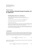
Figure 1: Flowchart of the proposed scheme.
and, therefore, the resulting substitute pixel set Z is filtered
using median operation, which is an L1 optimization in
Maximum Likelihood sense. Figure 1 shows the flow chart
of the proposed scheme.
There are several advantages of the proposed scheme. In
DBA the current noisy pixel under processing is replaced
with the median of the processing window. If the median
itself is corrupted, then the median is replaced by a previously
processed neighborhood pixel. At higher noise densities
most of the pixels will be corrupted necessitating repeated
replacement. This repeated replacement produces streaking.
The proposed method avoids this.
In robust statistics estimation filter [19–21], the current
noisy pixel under processing is replaced by an image data
estimated using an estimation algorithm. But the compu-
tation time is much longer. It will be demonstrated in
Section 7 that the linear prediction substitution followed by
median filtering as introduced by this paper can overcome
the problem of streaking and blur while the computational
complexity is reduced in comparison with robust statistics

estimation filter.
6. The Proposed Noise Removal Algorithm
Let X denote the image corrupted by salt and pepper noise.
For each pixel X(i, j), a 2-D sliding window of size 3
× 3is
selected in such a way that the current pixel lies at the centre
of the sliding window. The proposed algorithm first detects
the noisy pixel. If the current processing pixel lies inside the
dynamic range [0 255] then it is considered as a noise-free
pixel. Otherwise it is considered as a noisy pixel and replaced
by a value using the proposed linear prediction algorithm.
Step 1. A 2-D window “W
3×3
”ofsize3×3 is selected. Assume
that current pixel under processing is X(i, j).
Step 2. If 0 <X(i, j) < 255, X(i, j) is an uncorrupted pixel
and it is left unchanged and the window slides to the next
position.
Step 3. Else X(i, j) is a corrupted pixel and go to Step 10.
Step 4. Store all the elements of “W
3×3
”ina1-Darray“Y
A
”.
Step 5. Sort the 1-D array “Y
A
” in ascending order.
Step 6. For each pixel x(n)in“Y
A
” of value “255” moving

from left to right, replace x(n) by a predicted value which is
given by x(n)
= α · x(n − 1), where α = [R
xx
(1)/R
xx
(0)], 0 <
α<1 R
xx
(1), and R
xx
(0) are autocorrelation for lags 1 and 0.
Assuming stochastic approximation for maintaining sim-
plest computational complexity
R
xx
(
1
)
= x
(
n − 1
)
· x
(
n − 2
)
, R
xx
(

0
)
=
[
x
(
n
− 1
)
]
2
.
(9)
If α
= 0, substitute x(n)byx(n − 1). (Thisisaspecialcase
when the pixel x(n
− 2) is a salt noise pixel having the value
0.)
Step 7. For each pixel x(n)in“Y
A
” of value “0” moving from
right to left, replace x(n) by a predicted value which is given
by, x(n)
= α · x(n +1),whereα = [(R
xx
(1))/(R
xx
(0) )], 0 <
α<1,
R

xx
(
1
)
= x
(
n +1
)
· x
(
n +2
)
, R
xx
(
0
)
=
[
x
(
n +1
)
]
2
(10)
If α
≥ 1, substitute x(n)byx(n +1). ( T his is a special
case when the pixel x(n+2) is a pepper noise pixel having the
value 255.)

Step 8. The new array is Z
A
. Sort the 1-D array “Z
A
”with
predicted values and find the median value.
Step 9. Replace the current pixel X(i, j) under processing by
the above median value.
Step 10. Steps 1 to 3 are repeated until processing is
completed for the entire image.
7. Illustration of the Proposed Algorithm
Each and every pixel of the image is checked for the presence
of salt and pepper noise pixel. During processing if a pixel
element lies between “0 and 255”, it is left unchanged. If the
value is 0 or 255, then it is a noisy pixel and it is substituted
by a substitution pixel.
Array labeled Y
1
displays an image corrupted by salt and
pepper noise.
EURASIP Journal on Advances in Signal Processing 5
Array labeled Y
2
depicts the current processing window
and a pepper noise pixel. The square shown in solid
line represents the window ; and element inside the circle
represents a pepper noise pixel
199
234
255

178 189 160
188 205
255 255
255 255
255
200
169
255
0 0
210
20
168
0
0
0
0
Y
1
=
199
234
255
178 189 160
188 205
255 255
255 255
255
200
199
255

0 0
210
200
168
0
0
0
0
Y
2
=
If the current pixel under processing is between 0 and 255,
it is left unchanged. Otherwise it will be replaced by a new
pixel value estimated using the proposed algorithm. For
this purpose, the elements inside processing window are
arranged as an array Y
A
and sorted in ascending order
169 188 200 205 255 255 255 255 255
Y
A
=
169 188 200 205 200 255 255 255 255
Z
A
=
Check for the pixel elements of value “255” starting from
the left. If the pixel value is “255”, then that v alue will
be substituted by a predicted value from the immediate
neighborhood pixel. Array Z

A
illustrates this. The element
inside the circle is the substitute pixel for the pepper noise
pixel. This is repeated for all the pixels having the value “255”.
Array Z
A
is sorted again to find the median. This is shown as
array Z
D
. The element encircled is the median
169 188 200 200 200 200 205 205 205
Z
D
=
199
234
255
178 189 160
188 205
255 200
255 255
255
200
199
255
0 0
210
200
168
0

0
0
0
Z
P
=
Finally, the current noisy pixel in the window in array Y
2
is replaced with the new median value. The final processed
array is shown as Z
P
.
The element encircled in array Z
P
is the final estimate of
the pepper noise pixel of array Y
2
. In the proposed algorithm,
a3
× 3 window will slide over the entire image. Computation
complexity is minimum with a 3
× 3 fixed window. This
procedure is repeated for the entire image. Similar procedure
can be adopted for the salt noise substitution, estimation,
and replacement.
8. Simulation Results and Discussion
In this section, results are presented to illustrate the per-
formance of the proposed algorithm. Images are corrupted
by uniformly distributed salt and pepper noise at different
densities for evaluating the performance of the algorithm.

Three images are selected. They are Lena, Cameraman,
and Boat image. A quantitative comparison is performed
between several filters and the proposed algorithm in terms
of Peak Signal-to-Noise Ratio (PSNR), Mean Square Error
(MSE), Image Enhancement Factor (IEF), Mean Structural
SIMilarity (MSSIM) Index, and computational time. The
results show improved performance of the proposed algo-
rithm in terms of these measures. Matlab R2007b on a PC
equipped with 2.21 GHz CPU and 2 GB RAM has been used
for evaluation of computation time of all algorithms.
The performance of the algorithm for various images at
different noise levels from 70% to 90% is studied, and results
are shown in Figures 2–7. The metrics for comparison are
defined as follows:
PSNR
= 10 log 10

255
2
MSE

,
MSE
=
1
MN
M

i=1
N


j=1

rij − xij

2
,
IEF
=

M
i
=1

N
j
=1

n
ij
− r
ij

2

M
i=1

N
j=1


x
ij
− r
ij

2
,
SSIM
(
r, x
)
=

2μ
r
μ
x
+ C
1


2σ
xy
+ C
2


μ
r

2
+ μ
x
2
+ C
1

(
σ
r
2
+ σ
x
2
+ C
2
)
,
MSSIM
(
R, X
)
=
1
G
G

p=1
SSIM


r
p
, x
p

.
(11)
where r
ij
is the original image, x
ij
is the restored image,
and n
ij
is the corrupted image. The Structural SIMilarity
index between the original image and restored image is
given by SSIM [21]whereμ
r
and μ
x
are mean intensities
of original and restored images, σ
r
and σ
x
are standard
deviations of original and restored images, r
p
and x
p

are the
image contents of pth local window, and G is the number
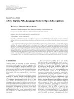
of local windows in the image. Figure 2 displays the original
and corrupted images of Lena.jpg image. Figure 4 displays
the original and corrupted images of Boat.gif image. Figure 6
displays the original and corrupted images of Cameraman.tif
image.
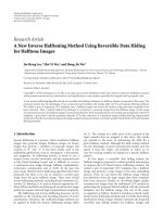
In Figures 3, 5 and 7, the first column represents the
output of Standard Median Filter (SMF) [4], second column
represents the output of Progressive Switching Median Filter
(PSMF) [14], third column represents the output of Adaptive
Median Filter (AMF) [16], and fourth column represents
the output of Decision-Based Algorithm (DBA) [17]. Fifth
column represents the output of Robust Estimation Median
Filter (REMF) [19] and the sixth column represents the
output of the Proposed Algorithm (PA). Tables 1–6 display
the quantitative measures. SMF replaces the current pixel
6 EURASIP Journal on Advances in Signal Processing
Table 1: PSNR and MSE for various filters for Lena image at different noise densities.
Noise density (%)
PSNR MSE
SMF PSMF AMF DBA REMF PA SMF PSMF AMF DBA REMF PA
20 29.039 32.379 37.561 37.476 38.204 40.188 81.126 37.6033 11.4017 11.6275 9.8338 9.1702
50 15.095 20.997 30.061 30.249 31.499 32.942 2011 9 516.869 64.1182 61.4046 46.050 41.5837
70 9.861 9.884 25.509 25.737 27.228 28.133 6713.6 6679.1 182.901 173.518 123.09 99.9569
80 7.926 7.983 22.975 22.936 24.702 25.836 10482 10346 327.752 330.747 220.25 169.607
90 6.441 6.485 19.283 19.770 21.355 24.316 14739 14609 767.042 685.698 476.01 240.925
Table 2: IEF and MSSIM for various filters for Lena image at different noise densities.
Noise density (%)
IEF MSSIM

SMF PSMF AMF DBA REMF PA SMF PSMF AMF DBA REMF PA
20 47.757 102.53 338.13 331.43 391.56 398.51 0.081 0.932 0.975 0.974 0.978 0.990
50 4.811 18.692 150.17 157.32 209.35 241.55 0.025 0.570 0.899 0.898 0.924 0.940
70 2.014 2.024 74.156 78.265 110.14 155.65 0.012 0.054 0.790 0.796 0.852 0.883
80 1.481 1.494 47.199 46.653 70.085 100.74 0.009 0.026 0.708 0.708 0.790 0.860
90 1.183 1.188 22.669 25.360 36.483 88.383 0.005 0.011 0.568 0.583 0.683 0.812
Table 3: PSNR and MSE for various filters for Boat image at different noise densities.
Noise density (%)
PSNR MSE
SMF PSMF AMF DBA REMF PA SMF PSMF AMF DBA REMF PA
20 27.091 30.110 34.840 34.706 35.256 38.428 127.06 63.396 21.334 22.004 19.387 16.632
50 15.074 20.406 27.820 27.842 28.985 31.393 2021.5 592.166 107.408 106.867 82.137 64.782
70 9.889 9.833 23.726 23.730 24.143 26.775 6671.3 6557.700 275.748 275.461 198.95 152.041
80 7.966 7.959 21.198 21.552 22.865 24.555 10388 10404.00 493.466 454.861 336.19 266.823
90 6.542 6.558 17.942 18.294 19.369 22.220 14416 14363.000 1044.500 963.108 751.93 389.985
Table 4:IEFandMSSIMforvariousfiltersforboatimageatdifferent noise densities.
Noise density (%)
IEF MSSIM
SMF PSMF AMF DBA REMF PA SMF PSMF AMF DBA REMF PA
20 30.185 59.774 176.77 172.65 196.61 204.95 0.109 0.918 0.970 0.970 0.973 0.982
50 4.685 15.975 88.062 88.574 115.02 126.85 0.035 0.576 0.879 0.878 0.903 0.951
70 1.989 1.974 47.993 48.274 66.722 77.234 0.017 0.065 0.754 0.756 0.807 0.912
80 1.466 1.464 30.766 33.230 45.331 53.011 0.011 0.032 0.657 0.665 0.726 0.839
90 1.184 1.186 16.361 17.689 22.783 41.416 0.007 0.016 0.518 0.531 0.600 0.787
Table 5: PSNR and MSE for var ious filters for Cameraman image at different noise densities.
Noise density (%)
PSNR MSE
SMF PSMF AMF DBA REMF PA SMF PSMF AMF DBA REMF PA
20 23.987 25.101 30.973 30.401 31.058 34.009 259.64 200.880 51.976 59.292 50.972 28.544
50 14.417 18.507 24.212 24.034 24.671 25.933 2351.5 917.025 246.554 256.824 221.80 147.737

70 9.455 9.397 20.944 20.580 21.893 23.686 7372.7 7471.200 523.252 568.926 420.55 297.153
80 7.768 7.719 18.328 18.621 19.659 22.700 10871. 10996.000 18.328 893.218 703.41 357.309
90 6.169 6.202 15.621 16.591 17.103 22.151 15711. 15592.000 1782.500 1425.600 1267.0 436.059
EURASIP Journal on Advances in Signal Processing 7
(a) (b) (c) (d)
Figure 2: (a) Original Lena image. (b) Image corrupted by 70% noise density. (c) Image corrupted by 80% noise density. (d) Image corrupted
by 90% noise density.
(a) (b) (c) (d) (e) (f)
Figure 3: Results of different filters for Lena image. (a) Output of SMF. (b) Output of PSMF. (c) Output of AMF. (d) Output of DBA. (e)
Output of REMF. (f) Output of PA. Row 1–Row 3 show processed results of various filters for Lena.jpg image corrupted by 70%, 80%, and
90% noise densities.
(a) (b) (c) (d)
Figure 4: (a) Original Boat image. (b) Image corrupted by 70% noise density. (c) Image corrupted by 80% noise density. (d) Image corrupted
by 90% noise density.
8 EURASIP Journal on Advances in Signal Processing
Table 6: IEF and MSSIM for various filters for cameraman image at different noise densities.
Noise density (%)
IEF MSSIM
SMF PSMF AMF DBA REMF PA SMF PSMF AMF DBA REMF PA
20 15.451 19.597 79.626 67.752 73.015 98.192 0.137 0.902 0.966 0.963 0.966 0.986
50 4.293 11.092 41.427 39.008 45.476 66.712 0.048 0.569 0.871 0.868 0.883 0.949
70 1.920 1.902 27.092 25.021 33.443 45.143 0.026 0.071 0.758 0.757 0.795 0.884
80 1.484 1.461 16.948 18.203 22.947 39.644 0.017 0.040 0.668 0.675 0.718 0.860
90 1.165 1.167 10.223 12.729 14.327 36.718 0.008 0.018 0.541 0.586 0.619 0.848
Table 7: Comparison of PSNR and CPU time in seconds for cameraman image.
Method
Noise density
= 70% Noise density = 80% Noise density = 90%
PSNR Time PSNR Time PSNR Time
SMF 9.8887 0.1043 7.9656 0.1055 6.5424 0.1111

Raymond H.Chan et al. 23.7257 38.4543 21.1982 44.4529 17.9415 51.0610
DBA 23.7302 5.6979 21.552 5.6357 18.2941 5.7585
REMF 24.1434 17.9368 22.8649 20.4194 19.369 23.0306
PA 26.7745 6.8083 24.5547 7.7198 22.2203 8.8524
(a) (b) (c) (d) (e) (f)
Figure 5: Results of different filters for Boat image. (a) Output of SMF. (b) Output of PSMF. (c) Output of AMF. (d) Output of DBA. (e)
Output of REMF. (f) Output of PA. Row 1–Row 3 show processed results of various filters for Boat.gif image corrupted by 70%, 80%, and
90% noise densities.
by its median value ir respective of whether a pixel is
corrupted or not. Therefore, the performance is poor. PSMF
has slightly improved performance but its noise removing
capacity is very poor at higher noise densities. AMF exhibits
improved performance but due to its adaptive nature the
computation complexity is much higher. DBA has very good
noise removing capability and good edge preservation at
higher noise densities but it produces streaking at higher
noise densities. REMF has improved performance than DBA
but its computational complexity is much higher. Figures
EURASIP Journal on Advances in Signal Processing 9
(a) (b) (c) (d)
Figure 6: (a) Original Cameraman image. (b) Image corrupted by 70% noise density. (c) Image corrupted by 80% noise density. (d) Image
corrupted by 90% noise density.
(a) (b) (c) (d) (e) (f)
Figure 7: Results of differentfiltersforCameramanimage.(a)OutputofSMF.(b)OutputofPSMF.(c)OutputofAMF.(d)OutputofDBA.
(e) Output of REMF. (f) Output of PA. Row 1–Row 3 show processed results of various filters for Cameraman.tif image corrupted by 70%,
80%, and 90% noise densities.
8–11 display the quantitative performance of the various
algorithms for cameraman image. It can be observed that the
proposed algorithm removes noise effectively even at higher
noise levels and preserves the edges and reduces streaking

which is a major drawback of DBA while maintaining
lower computational complexity when compared to adaptive
algorithm and robust statistics-based algor ithms. Figure 12
represents the computation time required at various noise
densities for different algorithms on cameraman image, and
the results are also tabulated in Tab le 7.
In the proposed method, replacement by immediate
neighborhood is avoided by substitution of noisy pixels
potential candidates based on linear prediction. Since linear
prediction is employed prior to any processing, repetition
of the same pixel is avoided as window is moved from one
position to the next position. This eliminates streaking. In
the standard switching median filtering except DBA, estima-
tion of noise-free pixels takes considerable time on account
of mathematical criteria employed. This time increases
significantly in adaptive based estimation techniques. In
the proposed filter, the estimation is not based on explicit
computation of estimation criteria; instead a median filtering
replaces estimation. This is the main reason for reduction in
computational complexity. Extra computation necessitated
by low-order linear prediction is significantly smaller than
techniques employing rigorous estimation schemes. The
DBA which is one of the fastest algorithms (which also
avoids estimation) involves three median sorting, namely,
right sorting, left, and diagonal sorting. In the proposed
filter there is only two sortings. Therefore introduction
10 EURASIP Journal on Advances in Signal Processing
Noise density versus PSNR
0
10

20
30
40
50
PSNR
10 20 30 40
50
60 70 80 90
Noise density (%)
SMF
PSMF
DBA
REMF
PAAMF
Figure 8: Noise density versus PSNR for cameraman image.
10 20
30 40
50 60 70 80 90
Noise density (%)
SMF
PSMF
DBA
REMF
PAAMF
0
1000
2000
3000
4000
5000

MSE
Noise density versus MSE
Figure 9: Noise density versus MSE for cameraman image.
10 20
30 40 50
60 70 80 90
Noise density (%)
SMF
PSMF
DBA
REMF
PA
AMF
Noise density versus IEF
0
20
40
60
80
100
120
IEF
Figure 10: Noise density versus IEF for cameraman image.
10 20 30 40 50 60 70 80 90
Noise density (%)
SMF
PSMF
DBA
REMF
PAAMF

0
0.2
0.4
0.6
0.8
1
MSSIM
Noise density versus MSSIM
Figure 11: Noise density versus MSSIM for Cameraman image.
10 20 30 40 50 60 70 80 90
Noise density (%)
SMF
PSMF
DBA
REMF
PAAMF
Noise density versus time
0
15
30
Time (seconds)
Figure 12: Noise density versus computation time in seconds for
Cameraman image.
of first-order linear prediction only slightly increases the
computation time compared with DBA but much lower
than other filters. The proposed algorithm can be a good
compromise in preference to the adaptive algorithm, DBA,
and robust statistics-based algorithm.
9. Conclusion
A new switching-based median filtering scheme and an

algorithm for removal of high-density salt and pepper noise
in images is proposed. The algorithm is based on a new
concept of substitution prior to estimation in contrast to the
standard switching-based nonlinear filters. Noisy pixels are
substituted by prediction prior to estimation. A simple novel
recursive linear predictor is developed for this purpose. A
subsequent optimization by median filtering results in final
estimates. The perfor m ance of the algorithm is compared
with that of SMF, PSMF, AMF, DBA, and REMF in terms
of Peak Signal-to-Noise Ratio, Mean Square Error, Mean
Structure Similarity Index, and Image Enhancement Factor
and Computational time. Both visual and quantitative results
EURASIP Journal on Advances in Signal Processing 11
are demonstrated. The results show that the notable features
of the proposed algorithm are reduced streaking at high
noise densities compared to DBA which is one of the fastest
algorithm and reduced computational complexity compared
to adaptive and robust algorithms. The proposed algorithm
can be a good compromise for salt and pepper noise removal
in images at high noise densities. However, further reduction
in computational complexity is desirable.
References
[1] I. Pitas and A. N. Venetsanopoulos, Nonlinear Digital Filters
Principles and Applications, Kluwer Academic Publishers,
Norwell, Mass, USA, 1990.
[2] J.AstolaandP.Kuosmanen,Fundamentals of Nonlinear Digital
Filtering, CRC Press, Boca Raton, Fla, USA, 1997.
[3] N. C. Gallagher Jr. and G. L. Wise, “A theoretical analysis of the
properties of median filters,” IEEE Transactions on Acoustics,
Speech, and Signal Processing, vol. 29, no. 6, pp. 1136–1141,

1981.
[4] T. A . Nodes and N. C. Gallagher Jr., “Median filters: some
modifications and their properties,” IEEE Transactions on
Acoustics, Speech, and Signal Processing, vol. 30, no. 5, pp. 739–
746, 1982.
[5] E. Abreu, M. Lightstone, S. K. Mitra, and K. Arakawa, “A
new efficient approach for the removal of impulse noise
from highly corrupted images,” IEEE Transactions on Image
Processing, vol. 5, no. 6, pp. 1012–1025, 1996.
[6] D.R.K.Brownrigg,“Theweightedmedianfilter,”Communi-
cations of the ACM, vol. 27, no. 8, pp. 807–818, 1984.
[7] O. Yli-Harja, J. Astola, and Y. Neuvo, “Analysis of the prop-
erties of median and weighted median filters using threshold
logic and stack filter representation,” IEEE Transactions on
Signal Processing, vol. 39, no. 2, pp. 395–410, 1991.
[8] G. R. Arce and J. L. Paredes, “Recursive weighted median
filters admitting negative weights and their optimization,”
IEEE Transactions on Signal Processing, vol. 48, no. 3, pp. 768–
779, 2000.
[9] Y. Dong and S. Xu, “A new directional weighted median filter
for removal of random-valued impulse noise,” IEEE Signal
Processing Letters, vol. 14, no. 3, pp. 193–196, 2007.
[10] T. Chen, K K. Ma, and L H. Chen, “Tri-state median filter for
image denoising,” IEEE Transactions on Image Processing, vol.
8, no. 12, pp. 1834–1838, 1999.
[11] H. Hwang and R. A. Haddad, “Adaptive median filters: new
algorithms and results,” IEEE Transactions on Image Processing,
vol. 4, no. 4, pp. 499–502, 1995.
[12] S. Zhang and M. A. Karim, “A new impulse detector for
switching median filters,” IEEE Signal Processing Letters, vol.

9, no. 11, pp. 360–363, 2002.
[13] H L. Eng and K K. Ma, “Noise adaptive soft-switching
median filter,” IEEE Transactions on Image Processing, vol. 10,
no. 2, pp. 242–251, 2001.
[14] Z. Wang and D. Zhang, “Progressive switching median filter
for the removal of impulse noise from highly corrupted
images,” IEEE Transactions on Circuits and Systems II, vol. 46,
no. 1, pp. 78–80, 1999.
[15] P E. Ng and K K. Ma, “A switching median filter with bound-
ary discriminative noise detection for extremely corrupted
images,” IEEE Transactions on Image Processing,vol.15,no.6,
pp. 1506–1516, 2006.
[16] R. H. Chan, C W. Ho, and M. Nikolova, “Salt-and-pepper
noise removal by median-type noise detectors and detail-
preserving regularization,” IEEE Transactions on Image Pro-
cessing, vol. 14, no. 10, pp. 1479–1485, 2005.
[17] K. S. Srinivasan and D. Ebenezer, “A new fast and efficient
decision-based algorithm for removal of high-density impulse
noises,” IEEE Signal Processing Letters, vol. 14, no. 3, pp. 189–
192, 2007.
[18] M. H. Hayes, Statistical Digital Signal Processing and Modeling,
John Wiley & Sons, Singapore, 2002.
[19] S. Schulte, M. Nachtegael, V. DeWitte, D. van der Weken, and
E. E. Kerre, “A fuzzy impulse noise detection and reduction
method,” IEEE Transactions on Image Processing,vol.15,no.5,
pp. 1153–1162, 2006.
[20] A. Ben Hamza and H. Krim, “Image denoising: a nonlinear
robust statistical approach,” IEEE Transactions on Signal
Processing, vol. 49, no. 12, pp. 3045–3054, 2001.
[21] Z. Wang, A. C. Bovik, H. R. Sheikh, and E. P. Simoncelli,

“Image quality assessment: from error visibility to structural
similarity,” IEEE Transactions on Image Processing, vol. 13, no.
4, pp. 600–612, 2004.