Báo cáo sinh học: " Research Article A Multifactor Extension of Linear Discriminant Analysis for Face Recognition under Varying Pose and Illumination" pdf
Bạn đang xem bản rút gọn của tài liệu. Xem và tải ngay bản đầy đủ của tài liệu tại đây (3.92 MB, 11 trang )
Hindawi Publishing Corporation
EURASIP Journal on Advances in Signal Processing
Volume 2010, Article ID 158395, 11 pages
doi:10.1155/2010/158395
Research Article
A Multifactor Extension of Linear Discriminant Analysis for Face
Recognition under Varying Pose and Illumination
Sung Won Park and Marios Savvides
Electrical and Computer Engineering Department, Carnegie Mellon University, 5000 Forbes Avenue Pittsburgh, PA 15213, USA
Correspondence should be addressed to Sung Won Park,
Received 11 December 2009; Revised 27 April 2010; Accepted 20 May 2010
Academic Editor: Robert W. Ives
Copyright © 2010 S. W. Park and M. Savvides. This is an open access article distributed under the Creative Commons Attribution
License, which permits unrestricted use, distribution, and reproduction in any medium, provided the original work is properly
cited.
Linear Discriminant Analysis (LDA) and Multilinear Principal Component Analysis (MPCA) are leading subspace methods for
achieving dimension reduction based on supervised learning. Both LDA and MPCA use class labels of data samples to calculate
subspaces onto which these samples are projected. Furthermore, both methods have been successfully applied to face recognition.
Although LDA and MPCA share common goals and methodologies, in previous research they have been applied separately and
independently. In this paper, we propose an extension of LDA to multiple factor frameworks. Our proposed method, Multifactor
Discriminant Analysis, aims to obtain multilinear projections that maximize the between-class scatter while minimizing the
withinclass scatter, which is the same core fundamental objective of LDA. Moreover, Multifactor Discriminant Analysis (MDA), like
MPCA, uses multifactor analysis and calculates subject parameters that represent the characteristics of subjects and are invariant
to other changes, such as viewpoints or lighting conditions. In this way, our proposed MDA combines the best virtues of both LDA
and MPCA for face recognition.
1. Introduction
Face recognition has significant applications for defense and
national security. However, today, face recognition remains
challenging because of large variations in facial image
appearance due to multiple factors including facial feature
variations among different subjects, viewpoints, lighting
conditions, and facial expressions. Thus, there is great
demand to develop robust face recognition methods that
can recognize a subject’s identity from a face image in
the presence of such variations. Dimensionality reduction
techniques are common approaches applied to face recog-
nition not only to increase efficiency of matching and
compact representation, but, more importantly, to highlight
the important characteristics of each face image that provide
discrimination. In particular, dimension reduction methods
based on supervised learning have been proposed and
commonly used in the foll ow ing manner. Given a set of face
images with class labels, dimension reduction methods based
on supervised learning make full use of class labels of these
images to learn each subject’s identity. Then, a generalization
of this dimension reduction is achieved for unlabeled test
images, also called out-of-sample images. Finally, these
test images are classified with respect to different subjects,
and the classification accuracy is computed to evaluate the
effectiveness of the discrimination.
Multilinear Principal Component Analysis (MPCA) [1,
2] and Linear Discriminant Analysis (LDA) [3, 4] are two
of the most widely used dimension reduction methods for
face recognition. Unlike traditional PCA, both MPCA and
LDA are based on supervised learning that makes use of given
class labels. Furthermore, both MPCA and LDA are subspace
projection methods that calculate low-dimensional projec-
tions of data samples onto these trained subspaces. Although
LDA and MPCA have different ways of calculating these
subspaces, they have a common objective function which
utilizes a subject’s individual facial appearance variations.
MPCA is a multilinear extension of Principal Com-
ponent Analysis (PCA) [5] that analyzes the interaction
between multiple factors utilizing a tensor framework. The
basic methodology of PCA is to calculate projections of data
samples onto the linear subspace spanned by the principal
directions with the largest variance. In other words, PCA
finds the projections that best represent the data. While PCA
2 EURASIP Journal on Advances in Signal Processing
calculates one type of low-dimensional projection vector for
each face image, MPCA can obtain multiple types of low-
dimensional projection vectors; each vector parameterizes
adifferent factor of variations such as a subject’s identity,
viewpoint, and lighting feature spaces. MPCA establishes
multiple dimensions based on multiple factors and then
computes multiple linear subspaces representing multiple
varying factors.
In this paper, we separately address the advantages and
disadvantages of multifactor analysis and discriminant anal-
ysis and propose Multifactor Discriminant Analysis (MDA)
by synthesizing both methods. MDA can be thought of as an
extension of LDA to multiple factor frameworks providing
both multifactor analysis and discriminant analysis. LDA
and MPCA have different advantages and disadvantages,
which result from the fact that each method assumes
different characteristics for data distributions. LDA can
analyze clusters distributed in a global data space based on
the assumption that the samples of each class approximately
create a Gaussian distribution. On the other hand, MPCA
can analyze the locally repeated distributions which are
caused by varying one factor under fixed other factors. Based
on synthesizing both LDA and MPCA, our proposed MDA
can capture both global and local distributions caused by a
group of subjects.
Similar to our MDA, the Multilinear Discr iminant
Analysis proposed in [6] applies both tensor frameworks
and LDA to face recognition. Our method aims to analyze
multiple factors such as subjects’ identities and lighting
conditions in a set of vectored images. On the other
hand, [6] is designed to analyze multidimensional images
with a single factor, that is, subjects’ identities. In [6],
each face image constructs an n-mode tensor, and the
low-dimensional representation of this original tensor is
calculated as another n-mode tensor with a smaller size. For
example, if we simply use 2-mode tensors, that is, matrices,
representing 2D images, the method proposed in [6]reduces
each dimension of the rows and columns by capturing the
repeated tendencies in rows and the repeated tendencies in
columns. On the other hand, our proposed MDA analyzes
the repeated tendencies caused by varying each factor in a
subspace obtained by LDA. The goal of MDA is to reduce the
impacts of environmental conditions, such as viewpoint and
lighting, from the low-dimensional representations obtained
by LDA. W hile [6] obtains a single tensor with a smaller
size for each image tensor, our proposed MDA obtains
multiple low-dimensional vectors, for each image vector,
which decompose and parameterize the impacts of multiple
factors. Thus, for each image, while the low-dimensional
representation obtained by [6] is still influenced by variance
in environmental factors, multiple parameters obtained by
our MDA are expected to be independent from each other.
The extension of [6] to multiple factor frameworks cannot
be simply drawn because this method is formulated only
using a single factor, that is to say, subjects’ identities. On
the other hand, our proposed MDA decomposes the low-
dimensional representations obtained by LDA into multiple
types of factor-specific parameters such as subject para-
meters.
The remainder of this paper is organized as follows.
Section 2 reviews subspace methods from which the pro-
posed method is der ived. Section 3 first addresses the advan-
tages and disadvantages of multifactor analysis and discrimi-
nant analysis individually, and then Section 4 proposes MDA
with the combined virtues of both methods. Experimental
results for face recognition in Section 5 show that the
proposed MDA outperforms major dimension reduction
methods on the CMU PIE database and the Extended Yale B
database. Section 6 summarizes the results and conclusions
of our proposed method.
2. Review of Subspace Projection Methods
In this section, we review MPCA and LDA, two methods
on which our proposed Multifactor Discriminant Analysis is
based.
2.1. Multilinear PCA. Multilinear Principal Component
Analysis (MPCA) [1, 2 ] is a multilinear extension of PCA.
MPCA computes a linear subspace representing the variance
of data due to the variation of each factor as well as the linear
subspace of the image space itself. In this paper, we consider
three factors: different subjects, viewpoints (i.e., pose types),
and lighting conditions (i.e., illumination). While PCA is
based on Singular Value Decomposition (SVD) [7], MPCA
is based on High-Order Singular Value Decomposition
(HOSVD) [8], which is a multidimensional extension of
SVD.
Let X be the m
p
× n data mat rix whose columns are
vectored training images x
1
, x
2
, , x
n
with n
p
pixels. We
assume that these data samples are centered at zero. By SVD,
the matrix X can be decomposed into three matrices U, S,
and V:
X
= USV
T
.
(1)
If we keep only the m<ncolumn vectors of U and V
corresponding to the m largest singular values and discard
the rests of the matrices, the sizes of the matrices in (1)areas
follows: U
∈ R
n
p
×m
, S ∈ R
m×m
,andV ∈ R
n×m
.Forasample
x, PCA obtains an m-dimensional representation:
y
PCA
= U
T
x.
(2)
Note that these low-dimensional projections preserve the dot
products of training images. We define the matr ix Y
PCA
∈
R
m×n
consisting of these projections obtained by PCA:
Y
PCA
= U
T
X = SV
T
.
(3)
Then, we can see that the Gram matrices of X and Y
PCA
are
identical since
G
= X
T
X = Y
T
PCA
Y
PCA
= VS
2
V
T
.
(4)
Since a Gram matrix is a matrix of all possible dot products, a
set of y
PCA
also preserves the dot products of original training
images.
EURASIP Journal on Advances in Signal Processing 3
While PCA parameterizes a sample x with one low-
dimensional vector y,MPCA[1] parameterizes the sample
using multiple vectors associated with multiple fac tors of
a data set. In this paper, we consider three factors of face
images: n
s
identities (or subjects), n
v
poses, and n
l
lighting
conditions. x
i,p,l
denotes a vectored training image of the
ith subject in the pth pose and the lth lighting condition.
These training images are sorted in a specific order so as to
construct a data matrix X
∈ R
m×n
s
n
v
n
l
:
X
=
x
1,1,1
, x
2,1,1
, , x
n
s
,1,1
, x
1,2,1
, , x
n
s
,n
v
,n
l
.
(5)
Using MPCA, an arbitrary image x and a data matrix X
are represented as
x
= UZ
v
subj
⊗ v
view
⊗ v
light
,(6)
X
= UZ
V
subj
⊗ V
view
⊗ V
light
T
,
(7)
respectively, where
⊗ denotes the Kronecker product and U
is identical to the matrix U in (1). A matrix Z results from
the pixel-mode flattening of a core tensor [1]. In (6), we
can see that MPCA parameterizes a single image x using
three parameters: subject parameter v
subj
∈ R
n
s
, viewpoint
parameter v
view
∈ R
n
v
, and lighting parameter v
light
∈ R
n
l
,
where n
s
≤ n
s
, n
x
≤ n
v
,andn
l
≤ n
l
. Similarly, X in (7)
is represented by three orthogonal matrices V
subj
∈ R
n
s
×n
s
,
V
view
∈ R
n
v
×n
v
,andV
light
∈ R
n
l
×n
l
. The columns of each
matrix span the linear subspace of the data space formed by
varying each factor . Therefore, V
subj
, V
view
,andV
light
consist
of eigenvectors corresponding to the largest eigenvalues of
three Gram-like matrices G
subj
, G
view
,andG
light
respectively,
where the (r, c) entry of these matrices is calculated as
G
subj
rc
=
1
n
v
n
l
n
v
p=1
n
l
l=1
x
T
r,p,l
x
c,p,l
,
G
view
rc
=
1
n
s
n
l
n
s
i=1
n
l
l=1
x
T
i,r,l
x
i,c,l
,
G
light
rc
=
1
n
s
n
v
n
s
i=1
n
v
p=1
x
T
i,p,r
x
i,p,c
.
(8)
These three Gram-like matrices G
subj
, G
view
, G
light
,represent
similarities between different subjects, different poses, and
different lighting conditions, respectively. For example, G
subj
can be thought of as the average similarity, measured by the
dot product, between the rth subject’s face images and the cth
subject’s face images under varying viewpoints and lig hting
conditions.
Three orthogonal matrices V
subj
, V
view
,andV
light
are
calculated by SVD of the three Gram-like matrices:
G
subj
= V
subj
S
subj
2
V
subj
T
,
G
view
= V
view
S
view
2
V
view
T
,
G
light
= V
light
S
light
2
V
light
T
.
(9)
Then, Z
∈ R
m
×n
s
n
v
n
l
can be easily derived as
Z
= U
T
X
V
subj
⊗ V
view
⊗ V
light
(10)
from (7). For a training image x
s,v,l
assigned as one column
of X, the three factor parameters v
subj
s
, v
view
v
,andv
light
l
are
identical to the sth row of V
subj
, vth row of V
view
,andl
th row of V
light
, respectively. In this paper, to solve for the
three parameters of an arbitrary unlabeled image x,onefirst
calculates the Kronecker product of these parameters using
(6):
v
subj
⊗ v
view
⊗ v
light
= Z
+
U
T
x,
(11)
where
+
denotes the Moore-Penrose pseudoinverse. To
decompose the Kronecker product of multiple parameters
into individual ones, two leading methods have been applied
in [2]and[9]. The best r ank-1 method [2] reshapes the
vector v
subj
⊗ v
view
⊗ v
light
∈ R
n
s
n
v
n
l
to the matrix
v
subj
(v
view
⊗ v
light
)
T
∈ R
n
s
×n
v
n
l
, and using SVD of
this mat rix, v
subj
is calculated as the left singular vector
corresponding to the largest singular value. Another method
is the rank-(1, 1, , 1) approximation using the alternating
least squares method proposed in [9]. In this paper, we
employed the decomposition method proposed in [2],
which produced slightly better performances for face
recognition than the method proposed in [9].
Based on the observation that the Gram-like matrices in
(8) are formulated using the dot products, Multifactor Kernel
PCA (MKPCA), a kernel-based extension of MPCA, was
introduced [10]. If we define a kernel function k, the kernel
versions of the Gram-like matrices in (8) can be directly
calculated. Thus, for training images, V
subj
, V
view
,andV
light
can be also calculated using eigen decomposition of these
matrices. E quations (10)and(11) show that in order to
obtain v
subj
, v
view
,andv
light
for any test image, also called
an out-of-sample image, x,wemustbeabletocalculate
U
T
X and U
T
x. Note that U
T
X and U
T
x are projections of
training samples and a test sample onto nonlinear subspace,
respectively, and these can be calculated by KPCA as shown
in [11].
2.2. Linear Discriminant Analysis. Since Linear Discriminant
Analysis (LDA) [3, 4] is a supervised learning algorithm,
class labels of all samples are provided to the traditional LDA
approach. Let l
i
∈ 1, 2, , c be the class label corresponding
to x
i
,wherei = 1, 2, , n and c is the number of classes.
Let n
i
be the number of samples in the class i such that
c
i=1
n
i
= n. LDA calculates the optimal projection direction
w maximizing Fisher’s criterion
J
(
w
)
=
w
T
S
b
w
w
T
S
w
w
,
(12)
where S
b
and S
w
are the between-class and within-class
scatter matrices:
S
b
=
c
i=1
n
i
(
m
i
− m
)(
m
i
− m
)
T
,
S
w
=
n
i=1
x
i
− m
l
i
x
i
− m
l
i
T
,
(13)
4 EURASIP Journal on Advances in Signal Processing
0
5
10
15
20
20
25
25
−5
−10
−15
0
5
10
15
−5
−10
−15
0
5
10
15
−5
−10
−15
−20
−25
(a)
0
5
10
15
20
20
25
25
−5
−10
−15
0
5
10
15
−5
−10
−15
0
5
10
15
−5
−10
−15
−20
−25
(b)
0
5
10
15
20
20
25
25
−5
−10
−15
0
5
10
15
−5
−10
−15
0
5
10
15
−5
−10
−15
−20
−25
(c)
0
5
10
15
20
20
25
−5
−10
−15
0
5
10
15
−5
−10
−15
0
10
−10
−20
−25
(d)
Figure 1: Low-dimensional representations of training images obtained by PCA using the CMU PIE database. (a) Each set of samples with
the same color represents each subject’s face images. (b) Each set of samples with the same color represents face images under each viewpoint.
(c) Each set of samples with the same color represents face images under each lighting condition. (d) The red C-shape curve connects face
images under various lighting conditions for one person and one viewpoint. The blue V-shape curve connects face i mages under various
viewpoints for one person and one lighting condition. Green dots represent 30 subjects’ face images under one viewpoint and one lighting
condition. We can see that varying viewpoints and lighting conditions create clusters, rather than varying subjects.
where m
i
denotes the sample mean for the class i.The
solution of (12) is calculated as the eigenvectors correspond-
ing to the largest eigenvalues of the following generalized
eigenvector problem:
S
b
w = λS
w
w.
(14)
Since S
w
does not have full column rank and thus is not
invertible, (14) can be solved not by eigen decomposition but
instead by a generalized eigenvector problem. LDA obtains a
low-dimensional representation y
LDA
for an arbitrary sample
x:
y
LDA
= W
T
x,
(15)
where the columns of the matr ix W
∈ R
n
p
×n
p
consist of
w
1
, w
2
, , w
p
. In other words, y
LDA
is the projection of x
onto the linear subspace spanned by w
1
, w
2
, , w
p
.Note
that p
<c. Despite the success of the LDA algorithm in
many applications, the dimension of y
LDA
∈ R
n
p
is often
insufficient for representing each sample. This is caused by
the fact that the number of available projection directions is
lower than the class number c. To improve this limitation of
LDA, variants of LDA, such as the null subspace algorithm
[12] and a direct L DA algorithm [13], were proposed.
3. Limitat i ons of Multifactor Analysis and
Discriminant Analysis
LDA and MPCA have different advantages and disadvan-
tages, which result from the fact that each method assumes
different characteristics for data distributions. MPCA’s sub-
ject parameters represent the average positions of a group of
subjects across varying viewpoints and lighting conditions.
EURASIP Journal on Advances in Signal Processing 5
Figure 2: Ideal factor-specific submanifolds in an entire manifold
on which face images lie. Each red cur ve connects face images
only due to vary ing viewpoint while each blue curve connects face
images only due to varying illumination.
MPCA’s averaging is premised on the assumption that these
subjects maintain similar relative positions in a data space
under each viewpoint and lighting condition. On the other
hand, LDA is based on the assumption that the samples
of each class approximately create a Gaussian distribution.
Thus, we can expect that the comparative performances of
MPCA and LDA vary with the characteristics of a data set.
For classification tasks, LDA sometimes outperforms MPCA;
at other times MPCA outperforms LDA. In this section, we
demonstrate the assumptions on which each method is based
and the conditions where one can outperform the other.
3.1. The Assumption of LDA: Clusters Caused by Different
Classes. Face recognition is a task to classify face images
with respect to different subjects. LDA assumes that each
class, that is, each subject, approximately causes a Gaussian
distribution in a data set. Based on this assumption, LDA cal-
culates a global linear subspace which is applied to the entire
data set. However, a real-world face image set often includes
other factors, such as viewpoints or lighting conditions
in addition to differences between subjects. Unfortunately,
the variation of viewpoints or lighting conditions often
constructs global clusters across the entire data set while
the variation of subjects creates only local distribution
as show n in Figure 1. In the CMU PIE database, both
viewpoints and lighting conditions create global clusters, as
shown in Figures 1(b) and Figure 1(c), while a group of
subjects creates a local distribution, as shown in Figure 1(a).
Therefore, low-dimensional projections obtained by LDA are
not appropriate for face recognition in these samples, which
are not globally separable.
LDA inspires multiple advanced variants such as Kernel
Discriminant Analysis (KDA) [14, 15], which can obtain
nonlinear subspaces. However, these subspaces are still based
on the analysis of the clusters distributed in a global data
space. Thus, there is no guarantee that KDA can be successful
if face images which belong to the same subjec t are scattered
rather than distributed as clusters. In sum, LDA cannot be
successfully applied unless, in a given data set, data samples
are distributed as clusters due to different classes.
3.2. The Assumption of MPCA: Repeated Distributions Caused
by Varying One Factor. MPCA is based on the assumption
that the variation of one factor repeats similar shapes of
distributions, and these common shapes rarely depend on
the variation of other factors. For example, the subject
parameters represent the averages of the relative positions
of subjects in the data space across varying viewpoints and
lighting conditions. To illustrate this, we consider viewpoint-
and lighting-invariant subsets of a given face image set; each
subset consists of the face images of n
s
subjects captured
under fixed viewpoint and lighting:
X
:,v,l
=
x
1,v,l
x
2,v,l
···x
n
s
,v,l
∈ R
n
p
×n
s
(16)
That is, each column of X
:,v,l
represents each image in this
subset. As shown in Figure 4(a), there are n
v
n
l
viewpoint-
and lighting-invariant subsets, and G
subj
in (8)canbe
rewritten as the average of the Gram matrices calculated in
these subsets:
G
subj
=
1
n
v
n
l
n
v
v=1
n
l
l=1
X
T
:,v,l
X
:,v,l
.
(17)
In Euclidean geometry, the dot product between two vectors
formulates the distance and linear similarity between them.
Equation (9) shows that G
subj
is also the Gram matrix of
a set of the column vectors of the matrix S
subj
V
subj
T
∈
R
n
s
×n
s
. Thus, these n
s
column vectors represent the average
distances between pairs of n
s
subjects. Therefore, the row
vectors of V
subj
, that is, the subject parameters, depend on
these average distances between n
s
subject across varying
viewpoints and lighting conditions. Similarly, the viewpoint
parameters and the lighting parameters depend on the
average distances between n
v
viewpoints and n
l
lighting
conditions, respectively, in a data space.
Figure 2 illustrates an ideal case to which MPCA can
be successfully applied. Face images lie on a manifold, and
viewpoint- and lighting-invariant subsets construct red and
blue curves, respectively. Each red curve connects face images
only due to varying illumination while each blue curve
connects face images only due to varying v iewpoints. Since
all of the red curves have identical shapes, n
l
different lighting
conditions can be perfectly represented by n
l
row v ectors of
V
light
∈ R
n
l
×n
l
. Also, since all of the blue curves have identical
shapes, n
v
different viewpoints can be perfectly represented
by n
v
row vectors of V
view
∈ R
n
v
×n
v
. For each factor,
when these subsets construct similar structures with small
variations, the average of these structures can successfully
cover each sample.
6 EURASIP Journal on Advances in Signal Processing
0
0
0
0
0
5
5
5
10
10
10
−5
−5
−10
0
−5
−5
−5
5
0
−5
0
−5
−10
−10
0
5
−5
−10
0
0
5
−5
−10
2
−4
5
5
10
5
0
−5
−5
−5
−10
10
5
0
−5
−10
10
15
15
20
10
10
5
15
20
0
10
5
15
20
0
0
10
10
5
15
20
0
10
5
15
20
10
5
15
20
20
0
10
20
0
10
5
15
20
10
5
15
20
0
10
5
15
20
10
5
15
20
0
10
5
15
20
20
20
25
10
5
15
20
25
10
5
15
20
0
10
5
15
20
(a)
−0.4
−0.3
−0.2
−0.1
−0.4
−0.3
−0.2
−0.1
0.1
0.2
0.3
0.4
−0.5
−0.5
0.5
0
0
(b)
0
5
−5
−5
−10
10
15
5
15
−15
0
5
−5
−10
10
15
−15
0
0
5
−5
−10
−10
10
10
15
−15
−15
−55
15
−15
−5
5
15−15
−5
5
15
−15
20
0
5
−5
−10
10
15
−15
20
20
10
20
25
−20
−20
0
5
−5
−10
10
15
−15
−20
0
5
−5
−10
10
−15
0
5
−5
−10
10
−15
−20
0
5
−5
−10
10
15
−15
−20
0
5
−5
−10
10
15
−15
−20
−20
0
−10−20
10
20
0
−10−20
10
20
0
−10
−20
−25
−5
5
15
−15
25
−25
(c)
−0.3
−0.2
−0.1
0.1
0.2
0.3
0.4
0
0
0.05
0.1
0.15
0.2
0.25
0.3
0.35
(d)
Figure 3: Low-dimensional representations of training images obtained by PCA and MPCA. (a) the PCA projections of 9 subjects’ face
images generated by varying viewpoints under one lighting condition. (b) the viewpoint parameters obtained by MPCA. (c) the PCA
projections of 9 subjects’ face images generated by var ying lighting conditions under one viewpoint. (d) the lighting parameters obtained by
MPCA.
We observe that each blue curve in Figure 3(a) that
represents viewpoint variation seems to repeat a similar
V-shape for each person and each lighting condition. Also,
Figure 3(b) visualizes the viewpoint parameters y
v
,learned
by MPCA; the curve connecting the viewpoint parameters
roughly fits the average shape of the blue curves. As a
result, y
v
in Figure 3(b) also has a V-shape. Also, the 3D
visualization of the lighting parameters in Figure 3(d)
roughly averages the C-shapes of red curves shown in
Figure 3(c), each connecting face images under various
lighting conditions for one person and one viewpoint.
Similar observations were illustrated in [9].
Based on the above expectations, if varying just one
factor generates dissimilar shapes of distribution, multilinear
subspaces based on these average shapes do not represent
a variety of data distributions. In Figure 3(a),somecurves
have W-shapes while most of the other curves have V-shapes.
Thus, in this case, we cannot expect reliable performances
from MPCA because the average shape obtained by MPCA
for each factor insufficiently covers individual shapes of
curves.
4. Multifactor Discriminant Analysis
As shown in Section 3.1, for face recognition, LDA is
preferred if in a given data set, face images are distributed
as clusters due to different subjects. Unlike LDA, as shown
in Section 3.2, MPCA can be successfully applied to face
recognition if various subjects’ face images repeat similar
shapes of distributions under each viewpoint and lighting,
EURASIP Journal on Advances in Signal Processing 7
even if these subjects do not seem to create these clusters. In
this paper, we propose a novel method which can offer the
advantages of both methods. Our proposed method is based
on an extension of LDA to multiple factor frameworks. Thus,
we can call our method Multifactor Discriminant Analysis
(MDA). From y
LDA
, MDA aims to remove the remaining
characteristics which are caused by other factors, such as
viewpoints and lighting conditions.
We start with the observation that MPCA is based on the
relationships between y
PCA
, low-dimensional representations
obtained by PCA, and multiple factor-specific parameters.
Combining (3)and(7), we can see that the matrix Y
PCA
∈
R
n
p
×n
s
n
v
n
l
is rewritten as
Y
PCA
= U
T
X = Z
V
subj
⊗ V
view
⊗ V
light
T
. (18)
Similarly, combining (2)and(7), for an arbitrary image x,
y
PCA
can be decomposed into three vectors by MPCA:
y
PCA
= U
T
x = Z
v
subj
⊗ v
view
⊗ v
light
T
(19)
where y
PCA
is the low-dimensional representation of x
obtained by PCA. Thus, we can think that Z performs a
linear transformation which maps the Kronecker product of
multiple factor-specific parameters to the low-dimensional
representations provided by PCA. In other words, y
PCA
is decomposed into v
subj
, v
view
,andv
light
by using the
transformation matrix Z.
In this paper, instead of decomposing y
PCA
, decomposing
y
LDA
is proposed, where y
LDA
is the low-dimensional repre-
sentation of x provided by LDA, as defined in (15). y
LDA
often
has more discriminant power than y
PCA
, but it still has the
combined characteristics caused by multiple factors. Thus,
we first formulate y
LDA
into the Kronecker product of the
subject, viewpoint, and lighting parameters:
y
LDA
= W
T
x = Z
v
subj
⊗ v
view
⊗ v
light
T
,
(20)
where W
∈ R
n
p
×n
p
is the LDA transformation matrix defined
in (14)and(15). As reviewed in Section 2.2, n
p
, the number
of available projection directions, is lower than the class
number n
s
: n
p
<n
s
. Note that y
LDA
in (20) is formulated in
a similar way to y
PCA
in (19) using different factor-specific
parameters and Z.Weexpectv
subj
in (20), the subject
parameter obtained by MDA, to be more reliable than both
y
LDA
and v
subj
since v
subj
provides the advantages of the
virtues of both LDA and MPCA. Using (15), we also calculate
the matrix Y
LDA
∈ R
n
p
×n
s
n
v
n
l
whose columns are the LDA
projections of training samples.
While MPCA decomposes the data matrix X
∈ R
n
p
×n
s
n
v
n
l
consisting of training samples, our proposed MDA aims to
decompose the LDA projection matrix Y
LDA
:
Y
LDA
= W
T
X = Z
V
subj
⊗ V
view
⊗ V
light
T
.
(21)
To obtain the factor-specific parameters of an arbitrary test
image x, we perform the following steps. During training,
we first calculate the three orthogonal matrices, V
subj
, V
view
,
and V
light
, and subsequently Z
. Then, during testing, for the
LDA projection y
LDA
of an arbitrary test image, we calculate
the factor-specific parameters by decomposing Z
+
y
LDA
.
In Section 3.2, factor-specific parameters obtained by
MPCA preserve the three Gram-like matrices G
subj
, G
view
,
and G
light
defined in (8). Figure 4 demonstrates that MPCA
calculates subject, viewpoint, and lighting parameters using
only the colored parts in the Gram matrix. These colored
parts represent the dot products between pairs of samples
that have only one varying factor. For example, the colored
parts in Figure 4(a) represent the dot products of different
subjects’ face images under fixed viewpoint and lighting
condition. Based on these observations, among the dot
products of pairs of LDA projections, we only use the dot
products which correspond to the colored parts of G in
Figure 4. Replacing x with y
LDA
, we define three new Gram-
like matrices, G
subj
, G
view
,andG
light
:
G
subj
m,n
=
n
v
v=1
n
l
l=1
y
T
LDAm,v,l
y
LDAn,v,l
,
=
n
v
v=1
n
l
l=1
x
T
m,v,l
WW
T
x
n,v,l
,
G
view
m,n
=
n
s
s=1
n
l
l=1
y
T
LDAs,m,l
y
LDAs,n,l
,
G
light
m,n
=
n
s
s=1
n
v
v=1
y
T
LDAs,v,m
y
LDAs,v,n
,
(22)
where y
LDAs,v,l
denotes the LDA projection of a training
image x
s,v,l
of the sth subject under the vth viewpoint and
the lth lighting condition. In (9), for MPCA, V
subj
, V
view
,
and V
light
are calculated as the eigenvector matrices of G
subj
,
G
view
,andG
light
, respectively. In similar ways, for MDA,
V
subj
∈ R
n
s
×n
s
, V
view
∈ R
n
v
×n
v
,andV
light
∈ R
n
l
×n
l
can
be calculated as the eigenvector matrices of G
subj
, G
view
,and
G
light
, respectively. Again, each row vector of V
subj
represents
the subject par ameter of each subject in a training set.
We remember that Y
LDA
∈ R
n
p
×n
s
n
v
n
l
and n
p
<n
s
.Thus,
if we define the Gram matrix G
as
G
= Y
T
LDA
Y
LDA
= X
T
WW
T
X,
(23)
this matrix G
∈ R
n
s
n
v
n
l
×n
s
n
v
n
l
does not have full column
rank. If G
is decomposed by SVD, G
has n
s
− 1nonzero
singular values at most. However, each of the matrices G
subj
,
G
view
,andG
light
has full column rank since these matrices
are defined in terms of the averages of different parts of G
as
shown in Figure 4.Thus,evenifn
p
<n
v
or n
p
<n
l
,onecan
calculate valid n
s
, n
v
,andn
l
eigenvectors from G
subj
, G
view
,
and G
light
,respectively.
After calculating these three eigenvector matrices, Z
∈
R
n
p
×n
s
n
v
n
l
can be easily calculated as
Z
= Y
LDA
V
subj
⊗ V
view
⊗ V
light
. (24)
8 EURASIP Journal on Advances in Signal Processing
S
1
S
1
S
2
S
2
(a) G (left) and G
subj
(right)
V
1
V
1
V
2
V
2
V
3
V
3
(b) G (left) and G
view
(right)
l
1
l
1
l
2
l
2
(c) G (left) and G
light
(right)
Figure 4: The relationships between the Gram matrix G defined in (4) and each of the Gram-like matrices G
subj
, G
view
,andG
light
defined
in (8), where a training set has two subjects, three viewpoints, and two lighting conditions. Each of G
subj
, G
view
,andG
light
is calculated as
the average of parts of the Gr am matrix G. Each entry of these three Gram-like matrices is the average of same-color entries of G.(a)G
subj
consists of averages of dot products which represent the averages of the pairwise relationships between a group of subjects. (b) G
view
consists
of averages of dot products which represent the averages of the pairwise relationships between different viewpoints. (c) G
light
consists of
averages of dot products which represent the averages of the pairwise relationships between different lighting conditions.
Thus, using this transformation matrix Z
, the Kronecker
product of the three factor-specific parameters is calculated
as
v
subj
⊗ v
view
⊗ v
light
= Z
+
y
LDA
.
(25)
Again, as done in (11), by SVD of the matrix v
subj
(v
view
⊗
v
light
)
T
, v
subj
is calculated as the left singular vector corre-
sponding to the largest singular value. Consequently, we can
obtain v
subj
of an arbitrary image test x.
5. Experimental Results
In this section, we demonstrate that Multifactor Discrim-
inant Analysis is an appropriate method for dimension
reduction of face images with varying factors. To test
the quality of dimension reduction, we conducted face
recognition tests. In all experiments, face images are aligned
using eye coordinates and then cropped. Then, face images
were resized to 32
× 32 gray-scale images, and each vectored
image was normalized with unit norm and zero mean. After
aligning and cropping, the left and right eyes are located at
(9, 10) and (24, 10), respectively, in each 32
× 32 image.
For the face recognition experiments, we used two
databases: the Extended YaleB database [16] and the CMU
PIE database [17]. The Extended YaleB database contains
28 subjects captured under 64 different lighting conditions
in 9 different viewpoints. For each of the subjects, we used
all of the 9 viewpoints and the first 30 lighting conditions
to reduce time for experiments. Among the face images, we
used 10 lighting conditions in 5 viewpoints for each person
for training and all of the remaining images for testing.
Next, we used the CMU PIE database, which contains 68
individuals with 13 different viewpoints and 21 different
lighting conditions. Again, to reduce time for experiments,
we utilized 30 subjects. Also, we did not use two viewpoints:
the leftmost profile and the rightmost profile. For each
person, 5 lighting conditions in 5 viewpoints were used
for training and all of the remaining images were used for
testing. For each set of data, experiments were repeated
10 times using randomly selected lighting conditions and
viewpoints. The averages of the results were reported in
Tables 1 and 2.
We compare the performance of our proposed method,
Multifactor Discriminant Analysis, and other traditional
subspace projection methods with respect to dimension
EURASIP Journal on Advances in Signal Processing 9
1
1
1
1
1
1
1
1
1
1
1
1
1
1
1
1
1
1
1
1
1
1
1
1
1
1
1
1
1
1
1
1
111
1
1
1
1
1
1
1
1
1
1
1
1
1
1
1
1
1
1
1
1
1
1
1
1
1
1
1
1
1
1
1
1
1
1
1
1
1
1
1
1
1
1
1
1
1
1
1
1
1
1
1
1
1
1
1
1
1
1
1
1
1
1
1
1
1
2
2
2
2
2
2
2
2
2
2
2
2
2
2
2
2
2
2
2
2
2
2
2
2
2
2
2
2
2
2
2
2
22
2
2
2
2
2
2
2
2
2
2
2
2
2
2
2
2
2
2
2
2
2
2
2
2
2
2
2
2
2
2
2
2
2
2
2
2
2
2
2
2
2
2
2
2
2
2
2
2
2
2
2
2
2
2
2
2
2
2
2
2
2
2
2
2
2
2
3
3
3
3
3
3
3
3
3
3
3
3
3
3
3
3
3
3
3
3
3
3
3
3
3
3
3
3
3
3
3
33
3
3
3
3
3
3
3
3
3
3
3
3
3
3
3
3
3
3
3
3
3
3
3
3
3
3
3
3
3
3
3
3
3
3
3
3
3
3
3
3
3
3
3
3
3
3
3
3
3
3
3
3
3
3
3
3
3
3
3
3
3
3
3
3
3
3
3
4
4
4
4
4
4
4
4
4
4
4
4
4
4
4
4
4
4
4
4
4
4
4
4
4
4
4
4
4
4
4
4444
4
4
4
4
4
4
4
4
4
4
4
4
4
4
4
4
4
4
4
4
4
4
4
4
4
4
4
4
4
4
4
4
4
4
4
4
4
4
4
4
4
4
4
4
4
4
4
4
4
4
4
4
4
4
4
4
4
4
4
4
4
4
4
4
4
5
5
5
5
5
5
5
5
5
5
5
5
5
5
5
5
5
5
5
5
5
5
5
5
5
5
5
5
5
5
5
5
555
5
5
5
5
5
5
5
5
5
5
5
5
5
5
5
5
5
5
5
5
5
5
5
5
5
5
5
5
5
5
5
5
5
5
55
5
5
5
5
5
5
5
5
5
5
5
5
5
5
5
5
5
5
5
5
5
5
5
5
5
5
5
5
5
6
6
6
6
6
6
6
6
6
6
6
6
6
6
6
66
6
6
6
6
6
6
6
6
6
6
6
6
6
6
666
6
6
6
6
6
6
6
6
6
6
6
6
6
6
6
6
6
6
6
6
6
6
6
6
6
6
6
6
6
6
6
6
6
6
6
6
6
6
6
6
6
6
6
6
6
6
6
6
6
6
6
6
6
6
6
6
6
6
6
6
6
6
6
6
6
6
7
7
7
7
7
7
7
7
7
7
7
7
7
7
7
7
7
7
7
7
7
7
7
7
7
7
7
7
7
7
7
7
7
7
7
7
7
7
7
7
7
7
7
7
7
7
7
7
7
7
7
7
7
7
7
7
7
7
7
7
7
7
7
7
7
7
7
7
7
7
7
7
7
7
7
7
7
7
7
7
7
7
7
7
7
7
7
7
7
7
7
7
7
7
7
7
7
7
7
7
8
8
8
8
8
8
8
8
8
8
8
8
8
8
8
8
8
8
8
8
8
8
8
8
8
8
8
8
8
8
8
8
888
8
8
8
8
8
8
8
8
8
8
8
8
8
8
8
8
8
8
8
8
8
8
8
8
8
8
8
8
8
8
8
8
8
8
8
8
8
8
8
8
8
8
8
8
8
8
8
8
8
8
8
8
8
8
8
8
8
8
8
8
8
8
8
8
8
9
9
9
9
9
9
9
9
9
9
9
9
9
9
9
9
9
9
9
9
9
9
9
9
9
9
9
9
9
9
9
9
9
9
9
9
9
9
9
9
9
9
9
9
9
9
9
9
9
9
9
9
9
9
9
9
9
9
9
9
9
9
9
9
9
9
9
9
9
9
9
9
9
9
9
9
9
9
9
9
9
9
9
9
9
9
9
9
9
9
9
9
9
9
9
9
9
9
9
9
0
0
0
0
0
0
0
0
0
0
0
0
0
0
0
0
0
0
0
0
0
0
0
0
0
0
0
0
0
0
0
0
0
0
0
0
0
0
0
0
0
0
0
0
0
0
0
0
0
0
0
0
0
0
0
0
0
0
0
0
0
0
0
0
0
0
0
0
0
0
0
0
0
0
0
0
0
0
0
0
0
0
0
0
0
0
0
0
0
0
0
0
0
0
0
0
0
0
0
0
−0.5
−0.4
−0.3
−0.2
−0.1
0
0.1
0.2
0.3
0.4
0.5
−0.4 −0.3
−0.2 −0.10 0.10.20.30.4
0.5
0.6
(a)
1
1
1
1
1
1
1
1
1
1
1
1
1
1
1
1
1
1
1
1
1
1
1
1
1
1
1
1
1
1
1
1
1
1
1
1
1
1
1
1
1
1
1
1
1
1
1
1
1
1
1
1
1
1
1
1
1
1
1
1
1
1
1
1
1
1
1
1
1
1
1
1
1
1
1
1
1
1
1
1
1
1
1
1
1
1
1
1
1
1
1
1
1
1
1
1
1
1
1
1
2
2
2
2
2
2
2
2
2
2
2
2
2
2
2
2
2
2
2
2
2
2
2
2
2
2
2
2
2
2
2
2
2
2
2
2
2
2
2
2
2
2
2
2
2
2
2
2
2
2
2
2
2
2
2
2
2
2
2
2
2
2
2
2
2
2
2
2
2
2
2
2
2
2
2
2
2
2
2
2
2
2
2
2
2
2
2
2
2
2
2
2
2
2
2
2
2
2
2
2
3
3
3
3
3
3
3
3
3
3
3
3
3
3
3
3
3
3
3
3
3
3
3
3
3
3
3
3
3
3
3
3
3
3
3
3
3
3
3
3
3
3
3
3
3
3
3
3
3
3
3
3
3
3
3
3
3
3
3
3
3
3
3
3
3
3
3
3
3
3
3
3
3
3
3
3
3
3
3
3
3
3
3
3
3
3
3
3
3
3
3
3
3
3
3
3
3
3
3
3
4
4
4
4
4
4
4
4
4
4
4
4
4
4
4
4
4
4
4
4
4
4
4
4
4
4
4
4
4
4
4
4
4
4
4
4
4
4
4
4
4
4
4
4
4
4
4
4
4
4
4
4
4
4
4
4
4
4
4
4
4
4
4
4
4
4
4
4
4
4
4
4
4
4
4
4
4
4
4
4
4
4
4
4
4
4
4
4
4
4
4
4
4
4
4
4
4
4
4
4
5
5
5
5
5
5
5
5
5
5
5
5
5
5
5
5
5
5
5
5
5
5
5
5
5
5
5
5
5
5
5
5
5
5
5
5
5
5
5
5
5
5
5
5
5
5
5
5
5
5
5
5
5
5
5
5
5
5
5
5
5
5
5
5
5
5
5
5
5
5
5
5
5
5
5
5
5
5
5
5
5
5
5
5
5
5
5
5
5
5
5
5
5
5
5
5
5
5
5
5
6
6
6
6
6
6
6
6
6
6
6
6
6
6
6
6
6
6
6
6
6
6
6
6
6
6
6
6
6
6
6
6
6
6
6
6
6
6
6
6
6
6
6
6
6
6
6
6
6
6
6
6
6
6
6
6
6
6
6
6
6
6
6
6
6
6
6
6
6
6
6
6
6
6
6
6
6
6
6
6
6
6
66
6
6
6
6
6
6
66
6
6
6
6
6
6
6
6
7
7
7
7
7
7
7
7
7
7
7
7
7
7
7
7
7
7
7
7
7
7
7
7
7
7
7
7
7
7
7
7
7
7
7
7
7
7
7
7
7
7
7
7
7
7
7
7
7
7
7
7
7
7
7
7
77
7
7
7
7
7
7
7
7
7
7
7
7
7
7
7
7
7
7
7
7
7
7
7
7
7
7
7
7
7
7
7
7
7
7
7
7
7
7
7
7
7
7
8
8
8
8
8
8
8
8
8
8
8
8
8
8
8
8
8
8
8
8
8
8
8
8
8
8
8
8
8
8
8
8
8
8
8
8
8
8
8
8
8
8
8
8
8
8
8
8
8
8
8
8
8
8
8
8
8
8
8
8
8
8
8
8
8
8
8
88
8
8
8
8
8
8
8
8
8
8
8
8
8
8
8
8
8
8
8
8
8
8
8
8
8
8
8
8
8
8
8
9
9
9
9
9
9
9
9
9
9
9
9
9
9
9
9
9
9
9
9
9
9
9
9
9
9
9
9
9
9
9
9
9
9
9
9
9
9
9
9
9
9
9
9
9
9
9
9
9
9
9
9
9
9
9
9
9
9
9
9
9
9
9
9
9
9
9
9
9
9
9
9
9
9
9
9
9
9
9
9
9
9
9
9
9
9
9
9
9
9
9
9
9
9
9
9
9
9
9
9
0
0
0
0
0
0
0
0
0
0
0
0
0
0
0
0
0
0
0
0
0
0
0
0
0
0
0
0
0
0
0
0
0
0
0
0
0
0
0
0
0
0
0
0
0
0
0
0
0
0
0
0
0
0
0
0
0
0
0
0
0
0
0
0
0
0
0
0
0
0
0
0
0
0
0
0
0
0
0
0
0
0
0
0
0
0
0
0
0
0
0
0
0
0
0
0
0
0
0
0
0.6
0.5
0.4
0
.3
0.2
0.1
0.1
0
−0.4
−0.3
−0.2
−0.1
−0.9 −0.8 −0.7 −0.6 −0.5 −0.4 −0.3 −0.2 −0.10
(b)
Figure 5: Two dimensional projections of 10 classes in the Extended
Yale B database. (a) features calculated by LDA, (b) subject
parameters calculated by MDA.
reduction: PCA, MPCA, KPCA, and LDA. For PCA and
KPCA, we used the subspaces consisting of the minimum
numbers of eigenvectors whose cumulative energy is above
0.95. For MPCA, we set the threshold in pixel mode to
0.95 and the threshold in other modes to 1.0. KPCA used
RBF kernels with σ set to 100. We compared the rank-1
recognition rates of all of the methods using the simple
cosine distance.
As shown in Tables 1 and 2, our proposed method,
Multifactor Discriminant Analysis, outperforms the other
−1 −0.9 −0.8 −0.7
−0.6
−0.5
−0.6 −0.5
−0.4
−0.3
−0.2
−0.1
0
0.1
−0.4 −0.3 −0.2 −0.10
0.3
0.2
0.1
Test images
Person 1 with pose 8
Person 4 with pose 1
Figure 6: The first two coordinates of lighting feature vectors
computed by Multifactor Discriminant Analysis using the Extended
Yale database.
Table 1: Rank-1 recognition rate on the Extended YaleB database.
untrained untrained Untrained
lighting viewpoints viewpoints & lighting
PCA 0.87 ± 0.03 0.64 ± 0.03 0.59 ± 0.05
MPCA 0.90
± 0.01 0.70 ± 0.05 0.65 ± 0.06
KPCA 0.88
± 0.03 0.67 ± 0.04 0.64 ± 0.06
LDA 0.89
± 0.03 0.65 ± 0.03 0.62 ± 0.05
MDA 0.94
±0.03 0.77±0.04 0.70±0.05
methods for face recognition. This seems to be because Mul-
tifactor Discriminant Analysis offers the combined virtues of
both multifactor analysis methods and discriminant analysis
methods. Like multilinear subspace methods, Multifactor
Discriminant Analysis can analyze one sample in a multiple
factor framework, which improves face recognition perfor-
mance.
Figure 5 shows two dimensional projections of 10 sub-
jects under varying viewpoints and lighting conditions
calculated by LDA and Multifactor Discriminant Analysis.
For each image, while LDA calculated one kind of projection
vector as shown in Figure 5(a), Multifactor Discriminant
Analysis obtained individual projection vectors for subjects,
viewpoint and lighting. Among the factor parameters,
Figure 5(b) shows subject parameters obtained by MDA.
Since these parameters are independent from varying view-
points and lighting conditions, the subject parameters of
face images are distributed as clusters created by varying
subjects rather than the scattered results in Figure 5(a).For
the same reason, Tables 1 and 2 show that MPCA and
Multifactor Discriminant Analysis outperformed PCA and
LDA respectively.
10 EURASIP Journal on Advances in Signal Processing
Table 2: Rank 1 recognition rate on the CMU PIE database.
untrained untrained untrained
lighting viewpoints view points & lig hting
PCA 0.89 ± 0.06 0.70 ± 0.05 0.22 ± 0.05
MPCA 0.91
± 0.04 0.74 ± 0.05 0.24 ± 0.06
KPCA 0.91
± 0.04 0.73 ± 0.05 0.23 ± 0.06
LDA 0.90
± 0.06 0.72 ± 0.05 0.23 ± 0.05
MDA 0.96
±0.04 0.79±0.04 0.27±0.06
Also, Figure 6 shows the first two coordinates of the
lighting features calculated by Multifactor Discriminant
Analysis for the face images of two different subjects in
different viewpoints. These two-dimensional mappings are
continuously distributed with steadily varying lighting while
differences in subjects or viewpoint appear to be relatively
insignificant. For example, for both Person 1 in Viewpoint 8
and Person 4 in Viewpoint 1, the mappings for face images
that were lit from the subjects’ right side appear on the top
left-hand corner, while dark images appear on the top-right
corner; images captured under neutral lighting conditions
lie on the bottom right. On the other hand, any two images
captured under similar lighting conditions tend to be located
close to each other even if they are of different subjects in
different viewpoints. Therefore, we can conclude that the
lighting features calculated by our proposed MDA preserve
neighbors for lighting, which are captured under similar
lighting conditions.
6. Conclusion
In this paper, we propose a novel dimension reduction
method for face recognition: Multifactor Discriminant Anal-
ysis. Multifactor Discriminant Analysis can be thought of
as an extension of LDA to multiple factor frameworks
providing both multifactor analysis and discriminant anal-
ysis. Moreover, we have show n through experiments that
MDA extracts more reliable subjec t parameters compared
to the low-dimensional projections obtained by LDA and
MPCA. These subject parameters obtained by MDA rep-
resent locally repeated shapes of distributions due to dif-
ferences in subjects for each combination of other factors.
Consequently, MDA can offer more discriminant power,
making full use of both global distribution of the entire
data set and local factor-specific distribution. Reference [6]
introduced another method which is theoretically based on
both MPCA and LDA: Multilinear Discriminant Analysis.
However, Multilinear Discriminant Analysis cannot analyze
multiple factor frameworks, while our proposed Multifactor
Discriminant Analysis can. Relevant examples are shown in
Figure 5 where our proposed approach has been able to yield
a discriminative two dimensional subspace that can cluster
multiple subjects in the Yale-B database. On the other hand,
LDA completely spreads the data samples into one global
undiscriminative distribution of data samples. These results
show the dimension reduction power of our approach in
the presence of nuisance factors such as viewpoints and
lighting conditions. This improved dimension reduction
power will allow us to have reduced size feature sets (optimal
for template storage) and increased matching speed due
to these smaller dimensional features. Our approach is
thus attractive for robust face recognition for real-world
defense and security applications. Future work will include
evaluating this approach on larger data sets such as the CMU
Multi-PIE database and NIST’s FRGC and MBGC databases.
References
[1] M. A. O. Vasilescu and D. Terzopoulos, “Multilinear image
analysis for facial recognition,” in Proceedings of the Interna-
tional Conference on Pattern Recognition, vol. 1, no. 2, pp. 511–
514, 2002.
[2] M. A. O. Vasilescu and D. Terzopoulos, “Multilinear inde-
pendent components analysis,” in Proceedings of the IEEE
Computer Society Conference on Computer Vision and Pattern
Recognition, vol. 1, pp. 547–553, San Diego, Calif, USA, 2005.
[3] K. Fukunaga, Introduction to Statistical Pattern Recognition,
Academic Press, San Diego, Calif, USA, 2nd edition, 1999.
[4] A. M. Martinez and A. C. Kak, “PCA versus LDA,” IEEE
Transactions on Pattern Analysis and Machine Intelligence, vol.
23, no. 2, pp. 228–233, 2001.
[5] M. Turk and A. Pentland, “Eigenfaces for recognition,” Journal
of Cognitive Neuroscience, vol. 3, no. 1, pp. 71–86, 1991.
[6] S.Yan,D.Xu,Q.Yang,L.Zhang,X.Tang,andH J.Zhang,
“Multilinear discriminant analysis for face recognition,” IEEE
Transactions on Image Processing, vol. 16, no. 1, pp. 212–220,
2007.
[7]G.H.GolubandC.F.V.Loan,Matrix Computations,The
Johns Hopkins University Press, London, UK, 1996.
[8] L. De Lathauwer, B. De Moor, and J. Vandewalle, “A multi-
linear singular value decomposition,” SIAM Journal on Matrix
Analysis and Applications, vol. 21, no. 4, pp. 1253–1278, 2000.
[9] M. A. O. Vasilescu and D. Terzopoulos, “Multilinear projection
for appearance-based recognition in the tensor framework,” in
Proceedings of the IEEE International Conference on Computer
Vision (ICCV ’07), pp. 1–8, 2007.
[10] Y. Li, Y. Du, and X. Lin, “Kernel-based multifactor analysis for
image synthesis and recognition,” in Proceedings of the IEEE
International Conference on Computer Vision, vol. 1, pp. 114–
119, 2005.
[11] B. Scholkopf, A. Smola, and K R. Muller, “Nonlinear com-
ponent analysis as a kernel eigenvalue problem,” in Neural
Computation, pp. 1299–1319, 1996.
[12] X. Wang and X. Tang, “Dual-space linear discriminant analysis
for face recognition,” in Proceedings of the IEEE Computer Soci-
ety Conference on Computer Vision and Pattern Recognition,pp.
564–569, 2004.
[13] H. Yu and J. Yang, “A direct LDA algorithm for high dimen-
sional data-with application to face recognition,” Pattern
Recognition, pp. 2067–2070, 2001.
[14] G. Baudat and F. Anouar, “Generalized discriminant analysis
using a kernel approach,” Neural Computation, vol. 12, no. 10,
pp. 2385–2404, 2000.
[15] S. Mika, G. Ratsch, J. Weston, B. Scholkopf, and K R. Muller,
“Fisher discriminant analysis with kernels,” in Proceedings of
the IEEE Workshop on Neural Networks for Signal Processing,
pp. 41–48, 1999.
EURASIP Journal on Advances in Signal Processing 11
[16] K C. Lee, J. Ho, and D. J. Kriegman, “Acquiring linear
subspaces for face recognition under variable lighting,” IEEE
Transactions on Pattern Analysis and Machine Intelligence, vol.
27, no. 5, pp. 684–698, 2005.
[17] T. Sim, S. Baker, and M. Bsat, “The CMU pose, illumination,
and expression database,” IEEE Transactions on Pattern Anal-
ysis and Machine Intelligence, vol. 25, no. 12, pp. 1615–1618,
2003.