Radio Frequency Identification Fundamentals and Applications, Design Methods and Solutions

216
solution found is the optimum available, because the parameter space for optimisation and
analysis is large, multidimensional and heterogeneous.
A first system success design approach based on software tools for system analysis and
optimisation including automatic parameter variation and model generation seems to be
more sufficient. Important questions like if a specific application would work using RFID
technique or how to dimension and position antennas can be answered qualitatively and
quantitatively on virtual level without doing prototyping. This design approach could be
less time consuming and expensive as well as provide better results to work with.
2. System modelling
2.1 Transponder system
Transponder systems consist of different modules strongly dependent on application. The
tag comprises for example a RF front end (Fig.1), a protocol stack with different complexity
and different features, a state machine or a microcontroller, memory like EEPROM, RAM
and flash or an analogue or digital interface to connect different actuators and sensors.



Fig. 1. Block diagram of a whole transponder system including reader and tag
On reader side, there is also a RF front end, a protocol stack and an application
programming interface (API) to connect it to a computer or a middle ware. Furthermore,
there are the antennas for both reader and tag ideally customised for each application.
In general, the goal of system design is to ensure a requested functionality on a specified
link distance. On RFID level that means transferring enough energy from reader to tag
wirelessly and to ensure an uni- or bidirectional wireless data communication. Hence, two
objective functions, energy range and transponder signal range (Finkenzeller, 2007), can be
derived. Energy range stands for a maximum distance, where the tag gets enough energy
from the field generated by the reader. And transponder signal range means a distance
between both reader and tag, where the reader receives data error-free sent by the tag. Both

distances must exceed the requested link distance to get a working RFID system. For
optimisation on electrical level, two important parameters, tag voltage and demodulator
input voltage, are helpful for system evaluation.
2.2 Extracted parameters and parameter space
Principally, transponder system design is divided into different steps. These are the design
of the transmission channel, the RF front ends, the digital protocol units and the application.
There are many solutions for the RF front end and the digital protocol unit to meet different
RFID standards. And there are various vendors providing powerful IPs, ICs or software
packages. The design of these communication components is very challenging because of
Virtual Optimisation and Verification of Inductively Coupled Transponder Systems

217
low device count and form factor. That implies using almost non-complex circuits and low
power constraints in general. But mostly these demands are independent of particular
applications, why these components can be reused in many different applications.
In contrast to ICs and protocol based software, the transmission channel depends directly on
each application and must be customised for successful implementation. To do that, the
kind of application or its implemented functions are not in foreground for optimisation.
More important are derived system properties like variation parameters and constraints
(Table 1) divided into transmission channel, electrical and protocol-dependent parameters.

Transmission Channel Electrical Parameters Protocol
Antenna Reader Carrier Frequency
• Size (Min, Max) • Driver
Bandwidth
• Shape • Demodulator

• Material
Tag


Antenna Configuration
• Power Consumption

Environment
• Modulator


Parasitics

Table 1. Important parameters and constraints for system optimisation divided into
different categories
Antennas and its parameters size, shape and material belong to the transmission channel
category as well as its configuration due to translation and rotation. Antenna size can be
specified for example by inner and outer radius for round windings, antenna width, number
of turns and used wire diameter with and without insulation. Another important point is
the environment, in which the system should be implemented. There can be eddy current
losses because of metals and fluids nearby the antennas influencing the behaviour of the
transmission channel. The second category defines electrical system parameters for both
reader and tag. It comprises for example the driver voltage, maximum driver current or
demodulator input voltage of the reader and load, minimum and maximum voltage as well
as modulation index of the tag. Parasitics like ohmic losses of resonance capacitors, antennas
and input capacitance of the tag chip or internal resistance of the driver circuit are very
important to get sufficient results. Besides geometrical, material and electrical properties,
protocol specific characteristics like carrier frequency and bandwidth must be considered,
too. Finally, transmission channel design, which is in the fore, is on low physical level where
functions of upper protocol layers or application generally do not influence results directly.
However, there is a heterogeneous and multidimensional parameter space with different
parameter ranges as well as discrete or continuous parameter variation. Often objective
functions with local or global extremes exist and the effort for detection could be high.
2.3 Electrical and electromagnetic model

To consider all important parameters during system design, the question now is which models
can be used and how they should interact. Principally, there are two different models –
electromagnetic and electrical. An idealised electrical model is shown in Fig. 2 for general
discussions. It comprises a model for a reader with a voltage source and a series resonance
circuit as well as a tag with parallel resonance circuit. The resistor R
L
is the load of the tag.
Radio Frequency Identification Fundamentals and Applications, Design Methods and Solutions

218


Fig. 2. Idealised electrical model of a transponder system using inductive coupling
The transmission channel can be described by the impedance matrix

()
RLRR R
TLTTT
VRjL jM I
VjMRjLI
ωω
ωω
+−
⎡
⎤⎡ ⎤⎡⎤
=
⎢
⎥⎢ ⎥⎢⎥
−+
⎣

⎦⎣ ⎦⎣⎦
, (1)
where V
R
and V
T
are the voltages over the antennas. I
R
and I
T
are the currents through the
antennas.
For system design of passive tags, two objective functions are important. These are the
energy range and the transponder signal range (Finkenzeller, 2007). Energy range means the
maximal distance between reader and tag, where the tag can extract enough energy from the
field. Transponder signal range means the maximal distance, where the reader can receive
data error-free from the tag. The sensitivity of the demodulator is very important for the
transponder signal range. The goal is that energy range and transponder signal range
exceed the required minimum link distance after system optimisation.
To evaluate both energy range and transponder signal range, two objective functions can be
used on the electrical level. These are the transponder voltage (2) and the demodulator input
voltage (3) (Deicke et al., 2008a).

2
2
2()
RL
T
LLT
LT L T

T
jMIR
V
RR
RR L
L
ω
ω
ω
=
⎛⎞
++
⎜⎟
⎝⎠
(2)

[]
0
,
11
Re ( ) Re ( )
RR R
RL RLMod
VVR
ZZ ZZ
⎛⎞
Δ= −
⎜⎟
⎜⎟
⎡

⎤
⎣
⎦
⎝⎠
(3)
The real part of the impedance Z
R
is

[]
()
2
22
()
Re
()()
R R LR LT L
LT L T
M
ZRR RZ
RZ L
ω
ω
=+ + +
−− +
. (4)
Z
L
is the parallel connection of C
T

and R
L
. Z
L,Mod
is the parallel connection of C
T
and R
L,Mod
.
Whereby, R
L,Mod
is the load resistance during modulation. Furthermore, there are constraints
on the electrical model. These are the quality factor of the reader (5) and the transponder (6).
Generally, the quality factor is defined by the quotient of resonance frequency and
bandwidth.
Virtual Optimisation and Verification of Inductively Coupled Transponder Systems

219

0 R
R
LR R
L
Q
RR
ω
=
+
(5)


0
24222
0
2
24
TL
T
LLLTL TL
LR
Q
RRR R LR
ω
ω
=
+−−
(6)
Considering equation (1) to (6) and the discussion in previous sections, there are many
different variables that influence V
T
and ΔV
RR
. On the one side there are electrical
parameters characterising the transmission channel that depend on geometrical dimensions,
antenna configuration, antenna material and eddy current losses due to fluids or metals
nearby antennas. These parameters must be calculated by an electromagnetic model and
forwarded to the electrical model. If magnetic materials like ferrite cores or ferromagnetic
plates are placed inside or nearby antennas, magnetic field strength or antenna current must
also be considered because of saturation. Then, there is an additional loop-back between
electrical and electromagnetic model.
On the other side there are electrical components of resonance circuits like R

R
, C
R
and C
T

that depend on antenna and transmission channel parameters as well as system constraints
like bandwidth and quality factor. It follows that there is no closed solution available that
takes into account both electrical and electromagnetic model. Because of that, manual
optimisation is very difficult for experienced designers, as well. An exhausted search in that
large multidimensional parameter space is not possible mostly because of considering a vast
number of possibilities that would result in a lack of time. On manual optimisation only few
solutions can be verified. And as a result, it is not really sure if the solution found, is the
optimum for a particular application or not. That means the quality of the result can not be
estimated in a sufficient way.
2.4 Current approaches and its bottlenecks
For RFID system dimensioning and analysis, different approaches had been discussed in
literature. The selection of an adequate modelling approach depends on target-oriented use
of variation parameters for design and optimisation. There are algebraic and numerical
solutions in general. A well known work is (Grover, 2004) where many approximated
formulas are collected to calculate self and mutual inductance for many different coil types.
Using the approximated formulas for the electrical level from the application note (Roz,
1998) in combination with that work, simple system analysis can be done with an existing
transmission channel including antennas and antenna configuration. Youbok introduced
with (Youbok, 2003) a more detailed application note including formulas for most common
antenna shapes and basic electrical circuits. For some standardised systems including co-
axial antennas, no additional literature is necessary. Another interesting approach is
discussed in (Finkenzeller, 2007) where a solution is presented to find the optimum antenna
radius of reader for given read range and constant coil current. The reason is if the antenna
radius is too large, the field strength is too low even at a distance of 0 between reader and

tag antenna. And in the other way around, if the radius is too small, there is high field
strength at distance 0, but it falls in proportion to x
3
from nearby the reader antenna. So,
Finkenzeller explains that radius R and read range x should have the relation

2xR = . (7)
Radio Frequency Identification Fundamentals and Applications, Design Methods and Solutions

220
A question, that was not discussed, is if that formula is always true in free air independent
of tag load or tag antenna size and shape. Mostly, it should not work in metal or fluid
environments.
Another interesting approach also explained in (Finkenzeller, 2007) is to find the minimum
field strength at tag side to power a passive tag. Therefore, the mutual inductance M in
equation (2) is replaced by a simple approximation using magnetic field strength H. Then
the equation is solved for H. After that the minimum magnetic field strength H
min
can be
estimated by defining a minimum tag voltage V
T
and a load resistance R
L
. With that result,
the designer is able to dimension the reader of a system without any further relation to the
tag side. An independent development of both reader and tag is possible if H
min
is constant.
That approach seems to be good for basic analysis and optimisation if the antennas and the
antenna configuration are well known and less accuracy is accepted. If antennas are

unknown at the beginning of system design like it is the case for many new industrial or
medical applications, it is difficult to find an optimised system. One point, that would also
impede the use of that approach, is, that electromagnetic and electrical model are mixed and
used in one step. So, it is really hard to implement more model details in that closed formula
even to increase accuracy. And there is also no numerical solver that can be used for such a
mixed approach. It can not be considered in that way if data transfer works from tag to
reader or not, because even formulas for simple models will be very complex and difficult
to handle. Finally, that approach only helps to optimise energy range.
Besides these approaches with a reduced abstraction level, modelling using numerical
methods is another way to increase model accuracy and to finally find better solutions.
Therefore, specific computer-aided tools are used, like it is also done for many other problems
in physics or engineering. But many specific tools such as ANSYS (ANSYS, 2007), FEMM
(Meeker, 2006) or Spice (Quarles et al., 2005) only provide comprehensive functionalities for
analysis and optimisation on particular modelling levels like mechanical, electrical or
electromagnetic. Heterogeneous systems can not be analysed or optimised with one tool.
Another possibility for analysis and optimisation is the use of modelling languages like
VHDL-AMS or Verilog-A. These are used to model physical behaviour such as acoustic,
electrical, magnetic, mechanical, optical or thermal. Interactions between different
modelling levels can be considered as well. Another advantage in comparison to numerical
solvers like ANSYS is that modelling languages are standardised. Thus it can be used
independent of a particular simulator. A disadvantage is that detailed models are very
complex and handling these complex models is often not as good as using numerical
solvers. Two approaches using standardised modelling languages are explained in
(Beroulle, 2003) and (Soffke, 2007). Beroulle uses VHDL-AMS to model a transponder
system on system level with a carrier frequency of 2.45 GHz to validate system performance.
Soffke takes a similar approach for system analysis. He uses Verilog-A to model an
inductively coupled transponder system. System optimisations are done manually. That
means, found solutions can be close to an optimum, but it can not be evaluated easily if it is
the case. Mostly it remains a big uncertainty.
All these approaches have in common not to be a good choice for system analysis and

optimisation considering the whole transponder system and considering enough details in
electrical and electromagnetic models to get sufficient results. Either it can be used for system
analysis or to analyse parts of a whole system in detail without regard to interactions of other
parts. Additionally, system optimisation is not described to find best solutions for different
usage scenarios. Thus it is assumed to do it manually with all restrictions discussed above.
Virtual Optimisation and Verification of Inductively Coupled Transponder Systems

221
3. Virtual design approach
3.1 Objectives
From discussions above, objectives are derived for a virtual design approach that can be
used for active and passive inductively coupled transponder systems. There, the focus is on
antennas, transmission channels and its effects on the electrical level. Reader or tag antenna
or both should be optimised dependent on application-specific requirements like
geometrical, material or electrical properties and regarding whole system behaviour.
Interactions between electrical and electromagnetic level should also be considered. During
optimisation, a multidimensional and automatic parameter variation should be possible
using adapted optimisation algorithm to get really optimised solutions and results with
good quality. Besides pure optimisation, transponder systems should be analysed for
different usage scenarios and different environments. Additionally, coaxial and non-coaxial
antennas should be considered. That implies to move and rotate a tag in space for analysing
operating range. To do that comprehensive analysis and optimisation, different model types
should be selectable to choose between model accuracy, calculation time and possible model
details like adding metal plates, for example. Finally, the goal is to make available a first
system success design approach. This means that the first solution meets the requirements
and can be used in practice without further extensive prototyping.
3.2 Design approach
These objectives were realised in a stand-alone software tool called Transponder Calculation
Tool (TransCal) and introduced in (Deicke et al., 2008b). It was developed by the Fraunhofer
IPMS. TransCal comprises different known solvers for electrical and electromagnetic models

(Fig. 3.). These are closed formulas for electrical model and for ohmic losses of antennas
including skin effect and proximity effect (Deicke et al., 2008a). Additionally, there is an
adapted Neumann formula used for high speed calculation of self and mutual inductance
for coaxial and rotated antennas. And there are links to external numerical solvers like
FastHenry (Kamon et al., 1996) and Spice (Quarles et al., 2005). FastHenry is a 3D
electromagnetic solver based on the Partial Element Equivalent Circuit method. It can be
used to model arbitrary antenna configurations, 3D antennas or additional conductive
structures nearby the antennas like metal plates or even metal rims to analyse transponder
systems in a car or truck wheel, for example.



Fig. 3. Design approach for TransCal
Besides these algorithms needed for detailed modelling on both levels, a framework is used
to implement algorithms for analysis, optimisation and model coupling to form a system
simulation. The framework bases on C/C++ in connection with Microsoft Foundation
Radio Frequency Identification Fundamentals and Applications, Design Methods and Solutions

222
Classes to get a MS Windows compliant software tool with an appropriate graphical user
interface. TransCal comprises five components like it is shown in the block diagram of
Fig. 4. The analyser/optimiser module analyses and optimises different transponder
systems using parameter variations and search algorithms. Furthermore, an automated
model generator reorganises and adapts imported user defined netlists and generates
antenna models as well as additional conductive structures nearby antennas. The model
coupling module controls and synchronises different internal analytical algorithms and
external numerical solvers selected by user.




Fig. 4. Block diagram of TransCal
3.3 Input/Output parameters and Initialisation
The input of several user defined design tasks and the output of results are done with
graphical user interface. Input parameters are geometrical and material properties of the
antennas, variation ranges for optimisation and analysis as well as electrical properties.
General settings for optimisation, analysis as well as used solvers can be made, too. The
results are shown in a text-based output window and additionally stored in text files to
provide the possibility for import in external data analysis and graphing tools. Fig. 5 shows
a screenshot from TransCal with dialog-based input and text-based output. Each design is
saved in a project file including all input settings and results to reopen and work on later.
For defining parameter space, constant and variable parameters have to be set. Dimensions
such as inner radius, outer radius and width of antenna or antenna type, number of turns
and link distance are variable parameters. Considering the optimisation of one antenna,
there are five degrees of freedom (DOF). And considering an optimisation of two antennas,
there are nine DOF. As a result, a five- or nine-dimensional parameter space must be used.
That seems to be very complicated and time consuming for most optimisation algorithms.
An advantageous modification of that parameter space could be helpful to solve that
optimisation task more efficiently. The reduction of variation parameters is to the fore.
Principally, the variation of antenna geometry can be done by varying the number of turns if
the antenna type is defined. Additionally, a constant fill factor has to be assumed. That is
done by defining an outer diameter of the used wire including conductor and insulation.
Using that substitution, the number of DOF can be reduced. Considering one antenna, the
parameter space is reduced to one dimension assuming a constant link distance. And
considering two antennas, the parameter space is reduced to two. If the link distance is
variable, the number of DOF is increased by one. Considering objective functions V
T
and

Virtual Optimisation and Verification of Inductively Coupled Transponder Systems


223

Fig. 5. Graphical user interface of TransCal with dialog-based input and text-based output
ΔV
RR
versus the number of turns, the characteristic of these functions is concave. That can be
used later to simplify optimisation process, too.
Subsequent to the definition of variation parameters, the generation of the n-dimensional
mesh is done. The parameter space has discrete values excluding link distance. Each node of
the mesh corresponds to a transponder system comprising a complete parameter set.
3.4 Optimisation and analysis
Looking from implementation side, optimisation and analysis are closely related to each
other in general. The main difference is in generating new input parameters for system
simulation. On system analysis, all defined nodes must be considered. Instead, there is a
bigger parameter space on optimisation in general. Therefore, a more efficient algorithm is
needed to consider as few as possible nodes during that process to reduce overall
calculation time. The general flow, that was adapted from the well known simulation-based
optimisation approach (Carson & Maria, 1997), is shown in Fig. 6. The analyser/optimiser
module generates a new parameter set. First, electrical parameters of the transmission
channel are calculated using an electromagnetic solver. These are the inductance and ohmic
losses of the antennas as well as the mutual inductance. The impedance matrix is imported
in the electrical circuit subsequently. After additional adaptations of resonance capacitors
and quality factors, the objective functions V
T
and ΔV
RR
are calculated and imported in the
analyser/optimiser module. There, the results are evaluated and a new parameter set is
output. For optimisation, that loop is repeated until an optimised solution will be found for
a given parameter space. Calculation of transmission channel and electrical circuit is

controlled by the coupling module.
Radio Frequency Identification Fundamentals and Applications, Design Methods and Solutions

224


Fig. 6. Simulation-based flow for analyser and optimiser
During system optimisation the goal is to find an optimal parameter set for any particular
application with a minimum amount of computing resources and time. Therefore, it is
desired that not all possibilities are evaluated explicitly. Especially with complicated and
heterogeneous systems, optimisation could be a challenging part. Using simulation-based
optimisation, all nodes must be found that meet defined constraints for objective functions.
Fig. 7 depicts an example, where all systems are looked for that met constraints for objective
functions at a constant link distance. With that contour plot objective functions V
T
and ΔV
RR

are shown over the number of turns for reader N
R
and tag N
T
. The dash-point line is the
equipotential line for the minimum transponder voltage V
T,min
. All nodes on the left hand
side have a tag voltage that is at least the minimum value. The dashed line is the
equipotential line for the minimum demodulator input voltage V
RR,min
. All nodes enclosed

with that line have a demodulator input voltage that is at least the minimum value. The
intersection of both areas shows all transponder systems that fulfil requirements for energy



Fig. 7. 2-dimensional mesh for an optimisation task and marked sections where objective
functions V
T
and ΔV
RR
meet requirements
Virtual Optimisation and Verification of Inductively Coupled Transponder Systems

225
range and transponder signal range at a given link distance. For that design example, these
systems are optimal solutions. If the intersection comprises only one node, that node defines
the system with maximum link distance.
Applying introduced simplifications for variation parameters, the objective functions are
concave. Because of that, robust and simple gradient based search algorithm and logical
operations are used to find the intersection. To find the node with maximum link distance,
an additionally root finding algorithm was implemented. So, the overall optimisation task is
divided into different steps using different simple and robust algorithms. In addition to that
advanced optimisation method, a brute force method was implemented that considers all
nodes available. Many design examples had shown that calculation time of the advanced
method is less than 4% of the brute force method.
3.5 Model coupling
The coupling module controls and synchronises different calculation types selected by user
before starting analysis or optimisation. There are internal closed formulas and additionally
external numerical solvers that can be selected for each modelling level to adjust used model
accuracy and calculation time (Fig. 8). On the one side, it is possible only to use internal

closed formulas and analytical algorithms to speed up calculation. Thereby, less accuracy is
accepted. And on the other side, external numerical solvers can be used for both electrical
and electromagnetic model to get best accuracy. The communication between TransCal and
these external solvers are done using command and result files. At the moment, FastHenry
and Spice can be used. But if necessary, other simulators can be connected, too. A third way
is to mix internal algorithm and external solvers like it is shown in an example later.



Fig. 8. Model coupling module and connected solvers
The model for FastHenry simulator is generated by model generator of TransCal for each
simulation step, because of changing antenna geometry. Besides calculation of coaxial
antennas in free air, FastHenry additionally has the possibility to model non-coaxial
antennas concerning translation and rotation as well as 3D antennas. Furthermore, metal
plates inside or under each antenna as well as car or truck rims can be modelled regarding
its influence on transmission channel. If other conductive structures should be used in
models, model generator must be extended before. That can not be done by user.
Using Spice, different user defined netlists can be imported by TransCal to provide the
possibility to add particular components as well as to analyse different circuit concepts for
reader and tag. The electrical model is focused on low level such as transmission channel,
Radio Frequency Identification Fundamentals and Applications, Design Methods and Solutions

226
parasitic elements and dependencies of the whole system primarily. More complex
components are replaced by basic equivalent circuits. That concern to, for example, ICs of
reader and tag. Mostly, detailed descriptions of such ICs are not available for system design
and of course not needed for that task in most cases. Often, basic properties extracted from
datasheets can only be used. If internal IC behaviour is available, it can be used for
modelling and simulation, too. However, effort for modelling and simulation should be
considered in comparison to the gain on accuracy. Because of that, a good approach is to

consider different resonance circuits, parasitic elements and different possibilities to connect
the demodulator input as well as the tag IC. Fig. 9 shows an example for an extended
electrical model. There, additional parasitics are considered like R
CT
as ohmic losses of the
resonance capacitor of the tag and C
L
as the input capacitor of the tag IC. During analysis or
optimisation the imported netlist is parameterised again for each simulation step dependent
on changes of transmission channel.



V0 1 0 dc 0 ac 6
CCR 1 3 58n
LLR 3 4 30u
RRLR 4 5 0.3
RRR 5 0 2.2
LLT 8 7 440u
RRLT 7 5 5.4
CCT 8 20 3.68n
RRCT 20 5 5
RRL 8 5 8000
CCL 8 5 30p
KK1 LLR LLT 0.01

a) b)
Fig. 9. Circuit example a) and netlist b)
4. Examples
4.1 Basic optimisation

The first example shows basic optimisation functions of the introduced approach with more
details. There, reader and tag antenna geometry must be optimised regarding to a given
input parameter set (Table 2). It describes a passive transponder system for a standard ID
and sensor application compliant to ISO 18000-2 protocol. The reader antenna is a disc coil
and defined by inner radius, used wire including insulation as well as minimum and
maximum number of turns. Additionally, electrical parameters are defined for driver and
demodulator input as well as carrier frequency and bandwidth. Unlike reader antenna, a
maximum winding space is defined for tag antenna like it is often defined in applications. It
includes inner radius, outer radius and maximum antenna width. The tag antenna is a
multi-layer coil.
Additionally, the used wire is not defined. The wire diameter varies between 0.08 to
0.25 mm regarding to IEC 60317. The tag includes a front end IC IPMS_RFFE125 (FhG IPMS,
2007), a microcontroller MSP430F123 (Texas Instruments, 2004) and additional application-
specific components. The estimated load is 11 kΩ approximately.
With that input parameter set, a parameter range is defined to vary antenna geometry of
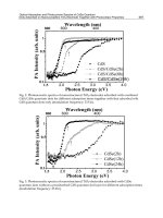
both reader and tag. In a first step V
T
and ΔV
RR
are calculated for different antenna
Virtual Optimisation and Verification of Inductively Coupled Transponder Systems

227
geometries at minimum link distance (Fig. 10). The wire diameter of tag antenna is 0.2 mm
in that case. Maximum values for V
T
and ΔV
RR
are not in the same region of parameter
space. So, the system with maximum transponder voltage or maximum demodulator input

voltage is not the system with maximum link distance.


Table 2. Input parameter set for reader and tag

a) b)
Fig. 10. Tag voltage V
T
a) and demodulator input voltage ΔV
RR
b) vs. number of turns for
reader and tag antenna at a fixed link distance
In a next step both antennas and system setup are optimised for maximum link distance
considering different wire diameters for tag antenna. The number of windings varies
between 21 and 22 for reader antenna, but there is no direct influence from wire diameter.
Fig. 11 a) shows the impedance of the tag antenna over the wire diameter for a constant
maximum winding space. The impedance for maximum link distance decreases with
Radio Frequency Identification Fundamentals and Applications, Design Methods and Solutions

228
increasing wire diameter, whereby ohmic losses decreases faster than inductance. As a
result, the quality factor increases, too. Mutual inductance has the same behaviour as self
inductance. So, the bigger losses because of smaller wire diameters are compensated by
increasing self and mutual inductances to an appropriate value. In the second diagram
(Fig. 11 b) the maximum link distance and the outer diameter of the tag antenna is shown.
Both parameters increase with wire diameter. The increase of the link distance from
0.08 mm to 0.25 mm is 34% approximately. But the increase of the outer diameter of tag
antenna is 6% only. Because of that, increasing wire diameter for a given winding space is a
good approach to maximise link distance without making tag antenna much bigger. But
finally, antenna optimisation is always a compromise between maximum antenna

dimensions, wire diameter, electrical system parameters and link distance.


a) b)
Fig. 11. Impedance of tag antenna a) as well as maximum link distance and outer diameter
b) vs. wire diameter of tag antenna
In a further discussion, the model accuracy and calculation time are compared for
introduced combinations of used solvers. Therefore, prototypes were made for reader
antenna and two tag antennas with wire diameter of 0.1 mm (MLC01) and 0.2 mm (MLC02).
The whole system was tuned to finally measure maximum link distance. During modelling,
the difference between link distance for MLC01 and MLC02 is 16.5%. In practice, difference
is 20.4%. If absolute values are considered, the maximum link distance differs between
12.1% for MLC02 and 16.3% for MLC01, whereby external simulators FastHenry and Spice
are used. Fig. 12 a) shows the error for calculating maximum link distance in relation to the
measured values of MLC02 over possible combinations of used solvers. On the one side, all
calculated values are bigger than the measured one. And on the other side, the error is
reduced by increasing model accuracy like mentioned before. But for coaxial antennas,
using Spice including a more detailed electrical circuit is more important than using
FastHenry instead of analytical formulas for the transmission channel.
If calculation time (Fig. 12 b) is also considered, the most efficient way is to use analytical
formulas for transmission channel and Spice for electrical circuit. That is a good compromise
between calculation error and time. Finally, the introduced approach of TransCal is good to
make a virtual design and to use the results qualitatively and quantitatively.
Virtual Optimisation and Verification of Inductively Coupled Transponder Systems

229

a) b)
Fig. 12. Calculated link distance in relation to measured a) and calculation time b) vs.
possible combinations of used solvers

4.2 3D antenna – dimensioning and analysis
Inductively coupled transponder systems are mostly analysed and optimised using coaxial
antennas. That approach is simple to use, but it is not sufficient for many applications and
its operating range or coverage. Because of that, analysis of tag rotation and translation is
important, too. In that section, analysis of rotation is in the fore. Standard antennas have a
limited coverage. However, 3D antennas with three coils assigned in perpendicular to each
other (Fig. 13), seem to have a better one. But a question is if 3D antennas will provide
power supply and communication for arbitrary rotation or not. Answers can be found by
making some analysis using TransCal.


Fig. 13. 3D antenna with perpendicular coils in the xy plane, the xz plane and the yz plane of
a Cartesian coordinate system
For modelling and optimisation of practical 3D antennas, different design constraints can be
used. The primary goal is to find a good approximation for geometrical and electrical
properties in comparison with a theoretical approach where three equal coils are used.
Therefore, design constraints are constant maximum link distance or constant coil
impedance. If the coils are optimised for constant impedance, the resonance circuits are
equal and as a consequence production process simplifies. Additional constraints are overall
dimensions of a 3D antenna that also influence the winding space of each coil.
Radio Frequency Identification Fundamentals and Applications, Design Methods and Solutions

230
If 3D antennas are generated using constant maximum link distance, V
T
and ΔV
RR
must
have the same values at the same link distance and same rotation approximately. Starting
from the inner coil that is also called basic antenna, the coil in the xz plane must have an

inner radius that is bigger than the outer radius of the basic antenna. In a second step, the
coil in the yz plane is generated, whereby its inner radius is bigger than the outer radius of
the coil in the xz plane. 3D antenna generation and optimisation is done by TransCal
automatically before starting further analysis. For that example a 3D antenna is derived
from MLC02. A model for FastHenry simulator is shown in Fig. 14.


Fig. 14. 3D antenna model for FastHenry simulator
The simulated coverage of the single antenna MLC02 and a derived 3D antenna are shown
in Fig. 15 over the rotation about the x axis (ϕ) and y axis (θ). Coverage means, where the
functionality of the tag is ensured. There, the transponder voltage V
T
and the demodulator
input voltage ΔV
RR
exceeds the defined limits at a given link distance. The coverage of the


a) b)
Fig. 15. Coverage of a single antenna a) and a 3D antenna b) vs. rotation about x axis (ϕ) and
y axis (θ)
Virtual Optimisation and Verification of Inductively Coupled Transponder Systems

231
single antenna is symmetric and represents 20.8% of the considered parameter space
approximately. In comparison, the 3D antenna has a coverage of 91.4% approximately. It is
more than 4.5 times bigger than of the single antenna. If link distance is very small, it could
be 100%. Finally, 3D antennas can be used to increase coverage if tag position is not defined
or if tag is rotating during use. But in most cases, 3D antennas are not able to get full
coverage during rotation.

4.3 Tags in truck or car tyres
The identification of a car or truck tyre with respect to manufacturer, type and mileage as
well as the measurement of physical parameters like pressure, temperature or stress during
use to warn against overstraining or damage (Lehmann, 2004) has been discussed
intensively for some time past. A passive and inductively coupled transponder system is
one possibility to realise that functionality, because it provides wireless energy transfer and
wireless data communication, less maintenance and the ability to integrate different sensors.
The properties of the transmission channel and the functionality of such a transponder
system depend on the rim material and shape as well as the dimensioning and the
positioning of both reader and tag antenna or using an additional steel cord. These
dependencies will be analysed in the following on a virtual level to evaluate system
usability and to derive important design rules concerning this usage scenario.
To realise the introduced application, a tag must be integrated in a tyre. The reader is
outside the tyre. Therefore, different types of antennas and antenna configuration had been
published in literature. Some examples are (Benedict, 2003), (Lehmann, 2004) and (Pollack,
2000). The used antennas and antenna configurations must ensure the functionality of the
tag independent of the size of the tyre, the speed of rotation and the position of the tag.
Because of that, an annular tag antenna is assumed to be for example under the tread



Fig. 16. Cross section of a wheel with integrated tag antenna and external reader antenna
Radio Frequency Identification Fundamentals and Applications, Design Methods and Solutions

232
(Fig. 16). The wheel and the tag antenna are coaxial. The annular antenna can be placed in
the middle of the tyre, nearby the sidewall or the bead as well as on the rim or directly on a
run-flat system (Continental, 2005; Rodgard, 2008). A steel cord can be placed inside the tyre
optionally. The rim model can be generated by TransCal automatically using different
variation parameters for a comprehensive analysis (Deicke et al., 2009).

The transponder circuit can also be placed under the tread or inside the tyre. The reader
antenna is outside and in parallel with the wheel. It is smaller than the tag antenna. So, the
reader antenna can be positioned on the axle or on an advantageous position in the wheel case.
A passive tag is used for identification and the integration of different sensors. Therefore,
the ST1 transponder IC is used in a test setup. It provides an analogue 125 kHz RF front-
end, a hard coded module to support low level ISO 18000-2 protocol functions, a 16-bit
microcontroller core, RAM, flash, EEPROM, timers and several peripheral components to
connect, for example, different sensors with an analogue or digital interface. Additionally,
analogue and digital signal processing can be done on the tag side (Grätz et al., 2007). In the
test setup, a combined pressure and temperature sensor MS5541 (Intersema, 2008) is
connected to the ST1. So, the power consumption of the passive tag can be estimated to use
it for analysing and optimisation of the whole system in the following. For system setup, the
general input parameters of Table 3 are used.


Reader Tag
r
i
31 mm r
i
243 mm
b 10 mm b 11 mm
N 56 N 33
Antenna
Parameters
Type MLC Type TWS
V
0
6.0 V V
T,min

5.0 V
ΔV
RR

0.01 V V
T,max
5.5 V
f
0
125 kHz R
L

14 kΩ
Electrical
Parameters
b
f
10 kHz R
L,Mod

30 Ω
Table 3. Input parameter set for reader and tag of a tyre application
Both reader and tag antenna are optimised for maximum link distance in free air. Then, this
optimised non-varying antenna setup is used to analyse and compare different rim
configurations with and without steel cord. Later, both antennas can be optimised
dependent on particular rim shape, size and material. The reader antenna is a multi-layer
coil (MLC). It is smaller than the tag antenna that is a thin-walled solenoid (TWS).
Additionally, Table 3 lists important electrical parameters of the reader and the tag.
Two parameters are very important for system evaluation if a transponder system is analysed
within a tyre. The first parameter is the minimum load resistance R

L,min
with a defined
transponder voltage and link distance. Therewith, the maximum power consumption can be
calculated to estimate which sensors and signal processing functions for measuring physical
parameters can be implemented into the tag. The second parameter is the demodulator input
voltage to determine if data communication is possible from tag to reader.
For the first analysis below, an antenna configuration is used without a steel cord. Thereby,
the rim width is varied to analyse different aspect ratios. Additionally, the reader antenna is
moved in radial direction starting from a coaxial position. With this example, the diameter
Virtual Optimisation and Verification of Inductively Coupled Transponder Systems

233
of the rim is 40 cm and the round plate of the rim is centred. The rim material is aluminium.
The diagrams of Fig. 17 a) and b) show the minimum load resistance and the demodulator
input voltage of the current setup with a link distance of 7.5 cm. The rim width is varied
from 1 cm to 10 cm. That corresponds to an aspect ratio from 4.3 to 0.43 including the range
of most used car and truck tyres. The reader antenna is moved in radial direction beyond
the tag antenna. The extremes of R
L,min
and ΔV
RR
are not with a coaxial antenna
configuration. They are at a radial shift of 19.3 cm approximately. If the reader antenna is
moved beyond the tag antenna, the load resistance increases sharply. ΔV
RR
has the same
behaviour in the opposite direction.

a) b)
Fig. 17. R

L,min
[kΩ] a) and ΔV
RR
[mV] b) vs. rim width and radial shift of the reader antenna
The diagrams also show, that R
L,min
and ΔV
RR
do not depend strongly on high rim widths.
As a result, low aspect ratios are not really an influencing factor with that configuration and
it can be assumed that the system would also work on lower values and flatter tyres
respectively. If a low rim width is considered, the distances between the round plate and the
antennas are smaller. So, the influence of the plate is bigger and for example on a coaxial
antenna configuration, the load resistance is bigger as on larger rim widths.
The diagram of Fig. 18 a) depicts the minimum load resistance versus the radial shift of the
reader antenna with different link distances and a constant rim width of 5 cm. The absolute
minimum value decreases and moves radially outwards with reducing link distance. So, it is
above the rim flange for very small distances. For example, considering a link distance of
2.5 cm, the minimum load resistance is at a radial shift of 21.8 cm approximately. If the link
distance increases, the absolute minimum also increases and moves towards the centre of
the rim. At a link distance of for example 15 cm, the minimum is at a radial shift of 13.3 cm.
At very high distances, the curve corresponds to a free air configuration without a metal rim
qualitatively. If the curve with a link distance of 2.5 cm is considered, the minimum of R
L,min

is 1.3 kΩ. For a link distance of 15 cm, the minimum is 11.3 kΩ. Thus the maximum power
consumption of the tag is 19.1 mW and 2.2 mW respectively if a transponder voltage of 5 V
is considered. This is sufficient to power the introduced passive tag for measuring pressure
and temperature. Considering the difference of R
L,min

between the centre position of the
reader antenna and the position of the absolute minimum value, it increases with reducing
the link distance. If the link distance is small, the correct position of the reader antenna is
more important than at higher link distances. The load resistance increases sharply if the
reader antenna is moved beyond the tag antenna.
Radio Frequency Identification Fundamentals and Applications, Design Methods and Solutions

234

a) b)
Fig. 18. R
L,min
vs. radial shift of the reader antenna for different link distances and a constant
rim width without a) and with steel cord b)
With a second analysis, the same configuration is considered with a steel cord, like it is
shown in Fig. 19. The steel cord is as wide as the rim and is 1 cm above the tag antenna. The
thickness is 2 mm. The diagram of Fig. 18 b) depicts the minimum load resistance versus the
radial shift of the reader antenna with different link distances, like it was done in the
analysis before. In comparison to Fig. 18 a), the curves are steeper and the range of radial
shift, where the tag would work, is smaller. Additionally, the minimum load resistance is
higher than without a steel cord. With a link distance of 15 cm, the tag can not be powered
from the RF field of the reader.

Fig. 19. FastHenry model of the transmission channel including the rim, a steel cord and the
antennas. The tag antenna is over the left rim flange.
Finally, the behaviour of an inductively coupled transponder system within a wheel setup
can be discussed before doing any prototyping. Whereby, analysis can be done for different
rim sizes and shapes, different reader and tag antennas, different antenna positions as well
as different electrical properties to find best solutions.
Virtual Optimisation and Verification of Inductively Coupled Transponder Systems


235
5. Conclusion
A first system success design approach for inductively coupled transponder systems was
introduced. It bases on a software tool called TransCal. This tool can be used for system
analysis and optimisation including automatic parameter variation and model generation.
Many different customised designs including RFID technique can be solved in an easy and
convenient way. Whereby, the focus is on transmission channel analysis, antenna design
and its effects on the electrical level. During design process, the system is divided in an
electromagnetic and an electrical model to consider necessary details in an appropriate way.
Therefore, analytical algorithms are implemented in TransCal. Additionally, external
numerical solvers can also be used to increase model accuracy. A model coupling module
controls and synchronises internal and external solvers for these modelling levels to provide
a system simulation finally. That functionality is used by an adapted simulation-based
optimisation algorithm to find optimised solutions in a large, multidimensional and
heterogeneous parameter space. In comparison to manual optimisation that only bases on
human experience, better results concerning quality and quantity can be found within less
amount of time. Using this approach, different usage scenarios can be considered such as
coaxial or non-coaxial antennas including rotation and translation, different environments
including eddy current losses as well as 3D antennas to increase tag coverage.
Besides the theoretical introduction, three design examples are presented to show the
advantages and limits of that approach. The first example introduces the basic optimisation
process considering accuracy and calculation time, too. The second example is an analysis of
3D antennas versus single-coil antennas to compare system behaviour during rotation. In a
third example a transponder system was implemented in a tyre for analysing different
antenna positions. Finally, important questions like if a specific application would work
using RFID technique or how to dimension and position antennas can be answered
qualitatively and quantitatively on virtual level without doing a lot of prototyping.
Additionally, it was shown that this design approach is less time consuming and expensive
as well as provide better results for LF and HF systems to work with.

6. References
ANSYS Inc. (2007). ANSYS 11.0 User Manual. www.ansys.com
Benedict, R.L. (2003). EPO Patent No. EP 1384603. European Patent Office
Beroulle V., Khouri R., Vuong T. & Tedjini S. (2003). Behavioral Modelling and Simulation of
Antennas: Radio-Frequency Identification case study. BMAS Conference 2003, pp.
102-106, San Jose, USA, October 2003
Carson, Y., Maria, A. (1997). Simulation Optimization: Methods and Applications. Winter
Simulation Conference of the INFORMS Simulation Society, Atlanta, Georgia,
December 1997
Continental AG. (2005). ContiSupportRing and Continental SSR. www.conti-online.com
Deicke, F., Grätz, H. & Fischer, W J. (2008a). Combined System Analyses and Automated
Design of RFID Transponder Systems. IEEE International Conference on RFID, pp.
328-335, Las Vegas, USA, April 2008
Deicke, F., Grätz, H. & Fischer, W J. (2008b). Computer-Aided Design of Antennas,
Transmission Channels and the Optimisation of Transponder Systems. RFID
SysTech 2008, pp. 32-41, June 2008
Radio Frequency Identification Fundamentals and Applications, Design Methods and Solutions

236
Deicke, F., Grätz, H. & Fischer, W J. (2009). Analysis of Antennas for Sensor Tags
Embedded in Tyres. RFID SysTech 2009, pp. 23-28, June 2009
FhG IPMS (2007). RFFE125 Datasheet.
applications/sas-info.shtml
Finkenzeller, K. (2007). RFID Handbook. Fundamentals and Applications in Contactless
Smart Cards and Identification. John Wiley & Sons Ltd.
Grätz, H, Heinig, A., Deicke, F. & Fischer, W.J. (2007). ST1 – ein freiprogrammierbarer
Schaltkreis für 125 kHz Transponderlösungen. Mikrosystemtechnik-Kongress,
Dresden, Germany, October 2007.
Grover, F. W. (2004). Inductance Calculations: Working Formulas and Tables. Reprinted in
Dover Publications

International Electrical Commission (2005). IEC 60317 Specifications for particular types of
winding wires. www.iec.ch
Intersema Sensoric SA (2008). MS5541-30C Datasheet.
products/guide/calibrated/ms55341-30c/
Kamon, M., Smithhilser, C., White, J. (1996). FastHenry User’s Guide.

Lehmann, J. (2004). WIPO Patent No. WO 2004/108439. World Intellectual Property
Organization
Meeker, D. (2006). Finite Element Method Magnetics User’s Manual ter-
miller.net
Pollack, R.S. (2000). EPO Patent No. EP 1037755. European Patent Office
Quarles, T., Pederson, D., Newton, R., Sangiovanni-Vincentelli, A. & Wayne, C. (2005). The
Spice Page. SPICE/
Rodgard (2008). Pneumatic Tire Run-Flat Systems. mobility.htm
Roz, T. & Fuentes, V. (1998). Using low power transponders and tags for RFID applications.
EM Microelectronic Marin SA
Soffke O., Zhao P., Hollstein T. & Glesner M. (2007). Modelling of HF and UHF RFID
Technology for System and Circuit Level Simulations. RFID SysTech 2007 - ITG-
Fachbericht Vol. 203. Duisburg, Germany, July 2007.
Texas Instruments (2004). MSP430x12x2 Datasheet. www.ti.com
Youbok, L. (2003). Antenna Circuit Design for RFID Applications. Microchip Technology
Inc.
14
Fabrication and Encapsulation Processes
for Flexible Smart RFID Tags
Estefania Abad
1
, Barbara Mazzolai
2
, Aritz Juarros

1
, Alessio Mondini
2
,
Angelika Krenkow
3
and Thomas Becker
1
Fundacion Tekniker, Eibar,
2
Scuola Superiore Sant’Anna, CRIM lab, Pisa,
3
EADS Deutschland GmbH, Innovation Works, München,
1
Spain
2
Italy
3
Germany

1. Introduction
RFID tags are often envisioned as a replacement for the current barcodes. These systems are
simple wireless transponders with integrated memory chips. Nowadays the challenge in
this field is the integration of sensors on board and there are some examples of tags in the
market including temperature and humidity sensors (Opasjumruskit et al. 2006). However,
there are no commercial labels containing chemical sensors. In this chapter book, we present
an integrated process flow for the integration of gas sensors onto flexible substrates together
with a RFID transponder to get a Flexible Tag Microlab (FTM) innovative system for food
logistic applications (see figure 1). In the proposed scenario, the FTM is designed to be
handled by a specifically designed reader with onboard sensing capabilities (Vergara et al.

2007). RFID technology in the 13.56 MHz band was chosen since it is the best compromise
for integration on a flexible tag. Furthermore this band is very suitable for the food logistic
application, considering possible constraints such us the surrounding environment (e.g.
humidity) and range of communication. In order to be compliant with recent RFID
developments the ISO 15693 standard has been selected.


Fig. 1. Main functional blocks of the FTM inlay for food logistics.
Radio Frequency Identification Fundamentals and Applications, Design Methods and Solutions

238
This visionary application involves both the fabrication of the so-called inlay, which is the
flexible substrate, acting mainly as a passive interconnect structure, with all components
needed for the FTM assembled on it, and the development of particular assembly and
packaging issues for the new ultra-low power consumption substrates for gas sensor
integration.
Flexible substrate, microcomponents assembly and encapsulation technologies have been
used throughout the electronics industry and continue to play a major role in new designs
and applications. Flexible substrate technologies refer to a group of processes for the
construction of multi-layer flexible circuits, commonly based on the use of a polyimide as
raw material. Typical fabrication of this type of circuit involves the masking and etching
methods similar to those employed by printed circuit board manufacturers. The component
assembly techniques have been developed to perform a hybrid integration of flexible
substrates with integrated electronic circuitry on bare dice. Flip chip bond, wire bond,
electrically conductive glues and tapes are some examples of connection methods.
Envisioned miniaturized systems could be assembled by combining these techniques and
solder steps. There is virtually no limit to the types of terminations possible for flexible
circuits. Wire, cable, contacts, printed circuit boards, chips and microstructures can be
connected to flex circuitry with these breakthrough technologies.
The process flow employed for the two metal levels interconnect fabrication will be

described in detail. The material used is the DuPont
TM
Pyralux® AP 8525R double-sided
copper-clad laminate, formed by a Kapton foil with a copper layer on each side. The vias
and windows openings are performed by femtosecond laser ablation. The copper
interconnections are realized by photolithography and wet chemical etching.
The MOX sensors hotplates specially developed to fulfil the FTM constrains in terms of low
power consumption has been used to prove two integration technologies into the flexible
substrates: Chip on Flex (COF) wire bonding and Anisotropic Conductive Adhesive (ACA)
flip chip bonding. Both technologies will be compared and benchmarked for future product
developments.
2. RFID flexible inlay fabrication
Flexible substrate and component assembly technologies (Numakura 2001) for the FTM
have been developed and/or optimised. Flexible circuit technology refers to a group of
additive or subtractive processes for the construction of multi-layers flexible circuits,
commonly based on the use of a polyimide (PI) as substrate. Specifically, two different
materials for substrates can been considered: DuPont Pyralux flexible composites and
photosensitive polyimide Pyralin PI2730 products.
Flexible composites technology uses Pyralux copper-clad laminated composites
1
, constituted
by DuPont Kapton polyimide film and copper foil on one or both sides, as flexible substrate.
The copper interconnections can be generated by standard photolithography (using either
DuPont adhesive photoresist coverlay that works as a negative photoresist or a positive
liquid photoresist) and wet etching. On the other hand, the vias definition in Kapton can be
performed either by photolithography and dry etching, or directly by femtosecond laser
ablation.

1


Fabrication and Encapsulation Processes for Flexible Smart RFID Tags

239
The main advantages of this technology are:
• Easy and quick to fabricate
• Good mechanical and electrical properties
• Low price
And the main drawbacks:
• Multilayer circuits need bonding and electrical contact trough vias.
On the other hand, there is the polymer thin film technology based on the use of
photosensitive polyimide. The polymer thin film represents an extension of the conventional
thin film technology. In this case, thin (< 20 μm) polymer dielectric films are deposited over
a substrate such us silicon. Then, a thin (< 2 μm) conductor layer, usually copper, is
deposited (PVD or CVD) and processed photolithographically. Vias can be easily achieved
by using a photopatternable polymer, as for example the Pyralin PI2730 products
2
. The
Pyralin PI2730 series are photosensitive negative working polyimides. Thin films of this
product can be applied by spin coating.
The main advantages of the thin film polymer technologies are:
• Narrow lines and vias
• Very high conductor a package density
• Very good mechanical and electrical properties of cured polyimide films
• Multilayer construction
And the main drawbacks:
• High cost
• Immature technology
A multiple spin steps process with the polyimide Pyralin PI2730 represents a powerful
solution for the fabrication of multilayer high density integrated circuits. The efficiency and
performance of this approach have been tested, comparing with the results obtained by an

approach based on the use of Pyralux double sided copper, in terms of feature size, time and
easiness of process. The results of this comparison activity (including advantages and
drawbacks of both the approaches) are briefly reported in the following:
• Pyralin PI2730, in a multilayer process configuration, allows a better integration of
complex circuits in a flexible tag.
• Pyralin PI2730 can be also used for developing the passivation layer.
• The approach based on Pyralin PI2730 shows a lower reproducibility in realizing planar
and homogeneous surfaces, when the flexible tag dimensions increase.
On the basis of the above mentioned results experimentally obtained, and considering the
low complexity of the tag circuits to be realized together with the usual dimensions of a
flexible Tag (credit card), the Pyralin based process is not necessary at this, and therefore the
Pyralux double sided copper was selected for developing the flexible tag.
A straightforward process flow for the fabrication of flexible substrates has been
implemented. The outline of this process is presented in the left part of Figure 2. The
material employed is the DuPont
TM
Pyralux® AP 8525R double-sided, copper-clad laminate
(Kapton), which is an adhesiveless laminate for flexible printed circuit applications. The
Kapton has a thickness of 50 µm and the copper layer has a thickness of 18 µm on each side.

2
Liquid Polyimide: Dupont Pyraline PI2730. http:://www.hdmicrosystems.com
Radio Frequency Identification Fundamentals and Applications, Design Methods and Solutions

240
In this procedure, the vias definition in Kapton was performed directly by femtosecond
laser ablation. Then, the copper interconnections of the two metal levels necessary for the
substrate were generated by standard photolithography and wet etching. Finally, contacting
through the vias was also implemented. Further details of this procedure are given
elsewhere (Abad et al. 2005). An example of the double sided flexible circuit (a) and antenna

(b) fabricated using this process is presented in the right part of Figure 2.


Fig. 2. Process design for flexible substrates fabrication, left image. Photographs and
microscope images of the flexible circuit (a) and the flexible antenna (b). Detail of the copper
tracks of the inductor.
Figure 3 shows a prototype of the developed FTM. The implemented system is a semi-active
tag with a passive read-out and a battery powered sensing part, as reported in (Zampolli et
al. 2007). The main functional blocks include a flexible antenna, a microcontroller for sensor
control and signal acquisition, a RFID front-end and a complex programmable logic device
(CPLD) for signal modulation/demodulation, commercial sensors (relative humidity,
temperature and light), an EEPROM memory and a thin film flexible battery. For this
prototype packaged chips were integrated on the flexible circuit using conventional
assembly technologies.
3. MOX sensors integration
The integration of MOX sensors on a flexible tag has several critical aspects, mainly due to
mechanical reliability and power consumption and requires specific assembling methods
and protection of the chips from the environment. The power consumption issues were
addressed in the design of Ultra-Low Power Hot Plates (ULPHP) but mechanical aspects