198 4. Market Definition
To help inform the analysis of the large amount of survey evidence considered in
that case, a summary of the evidence is presented in table 4.6. In particular, note that
the results of four separate surveys are reported. The surveys are called respectively
Swift 1, ORC, Swift 2, and GfK after the survey companies which undertook them.
The first two surveys were addressed toward customers who had recently stopped
playing with a provider (“lapsed” customers) while the second two surveys involved
current customers.
In terms of the latter pair of surveys, the Swift 2 survey asked consumers directly
how they would respond to a 10% price increase
29
while the GfK survey used show-
cards to allow consumers to compare hypothetical product offerings. The CC has
found that directly asking consumers about what they would do if prices went up
by 10% can sometimes lead to results that are difficult to interpret. Show cards can
also sometimes produce surprising results. For example, one part of the GfK survey
used show-cards and suggested increasing demand schedules!
Surveys aimed at capturing diversion ratios aim to directly estimate the substitu-
tion effect between two products. These methods have the merit that they address
directly the issue of interest in market definition and make few theoretical assump-
tions. But they are heavily reliant on good-quality data obtained through high-quality
surveys. Survey design in this area remains under development.
Wherever our information on substitution patterns comes from, surveys or demand
estimation, we will of course still need to use that information to evaluate the impor-
tance of rival products as constraints on price-setting behavior. In section 4.6, we
discuss strategies that can be used both quantitatively, when we have good-quality
data, but also sometimes qualitatively when we do not. Before we do so we first
turn briefly to one additional technique sometimes useful for geographic market
definition.
4.5 Using Shipment Data for Geographic Market Definition
Elzinger and Hogarty (1973, 1978)

30
proposed a two-stage test for geographic mar-
ket definition. The two stages are known respectively as “little out from inside”
(LOFI) and “little in from outside” (LIFOUT). Given a candidate market area, the
LIFOUT test considers whether nearly all purchases come from within the region
itself or whether there are substantial “imports.” Analogously, given a candidate
market area, the LOFI test considers whether nearly all shipments go to the region
itself or whether there are substantial “exports” from the region. Intuitively, import
and export activities suggest competitive interconnectivity. LOFI is also sometimes
29
The Swift 2 survey asked: “If your pools company increased the cost of playing by 10%, what would
you do?”
30
A nice description of the U.S. judicial history in this (and other) areas is provided by Blumenthal et
al. (1985). See also Werden (1981, pp. 82–85).
4.5. Using Shipment Data for Geographic Market Definition 199
described as the “supply” element of the test, since it relates particularly to the des-
tination of production coming from a candidate area, while LIFOUT is sometimes
considered as the “demand” element of the test since it relates to purchases made
by consumers in the candidate market area. The overall idea of the combined test
(LIFOUT + LOFI) is to expand the candidate market areas until both “supply” and
“demand” sides of the test are satisfied in a market area.
To operationalize this test, we must first define what we mean by “little.” Elzinga
and Hogarty suggested using benchmarks so that if only 25% (or they later suggested
10%) of production in an area is “exports” or “imports,” we would consider there
to be respectively LOFI or LIFOUT.
To apply the LOFI test, the authors suggest beginning with the largest firm or
plant and finding the area where (say) 25% of that plant’s shipments goes to. The
LOFI test then asks whether
LOFI D 1 

Shipments from plants in area to inside
Production in candidate area
D
Exports
Production in candidate area
6 0:25:
If so, then the LOFI test is met, since “nearly all” of the sales from plants occur
within the area. If the test fails, then area must be expanded to find an appropriate
area where the test is indeed satisfied. One option is to find the minimum area needed
to account for 75% of output from all plants within the previous candidate area. If
the expansion of the area does not involve incorporating any new plants, then such
a procedure clearly generates an area that will meet the LOFI test. On the other
hand, expanding to capture more sales of the set of plants under consideration may
sometimes also place additional plants within the candidate market area and we
shall return to this observation in a moment.
The LIFOUT test examines the purchase behavior of consumers within acandidate
region, asking whether
LOFOUT D 1 
Purchases by consumers in area
Production in candidate area
6 0:25:
In some contexts, particularly commodity markets, the Elzinga–Hogarty test has
been generally well received by government agencies, the courts, and the compe-
tition policy academic community over the last thirty years. However, in the late
1990s the test came under renewed scrutiny after the U.S. agencies and state author-
ities objected to seven out of a total of 900 hospital mergers between 1994 and 2000
and lost all seven of the cases! A number of these cases were lost because the courts
accepted the merging parties’ application of the Elzinga–Hogarty test using patient
flow data.
A period of reflection and retrenchment followed with the Federal Trade Com-

mission (FTC) and Department of Justice (DOJ) undertaking a major exercise of
200 4. Market Definition
hearings and consultation, summarized in FTC and DOJ (2004).
31
DOJ and FTC
concluded that “the Agencies’ experience and research indicate that the Elzinga–
Hogarty test is not valid or reliable in defining geographic markets in hospital merger
cases” (chapter 4, p. 5).
Proponents of the test would no doubt argue that this is in fact a fairly limited
conclusion, in particular perhaps noting that DOJ and FTC do not say that Elzinga–
Hogarty is not valid and reliable, only that it is not valid and reliable in hospital
mergers. However, at least these comments make the hospital context particularly
interesting and so we focus on it. In addition, it is difficult to escape the observation
that the primary critiques leveled at Elzinga–Hogarty in that context do appear to
apply far more widely.
To see how Elzinga–Hogarty was applied in hospital mergers, note that a patient
who lives in a candidate market area but who goes to a hospital outside it for
treatment is considered to be “importing” hospital services into the candidate area,
and is measured as LIFOUT since she is inside the area and purchasing hospital
services outside it. On the other hand, a patient who lives outside the candidate area
and who comes into the area to the hospital is considered an “export” of services
and so is measured as LOFI.
The first critique of the Elzinga and Hogarty test is that existing “flows” of supply
or demand need not be informative about market power. In particular, the fact that
some consumers currently use hospitals outside the area does not imply that the
level of “imports” would increase dramatically if hospitals within the market area
increased prices by a small amount. The FTC and DOJ go on to note that patients
travel for a number of reasons, including “perceived and actual variations in quality,
insurance coverage, out-of-pocket cost, sophistication of services, and family con-
siderations” (chapter 4, p. 8). If so, then the fact that some consumers travel does

not immediately imply that those who are currently not traveling are price-sensitive.
Capps et al. (2001) call this logical leap the “fallacy of the silent majority.”
The second critique noted that if LIFOUT or LOFI fail with a given candidate
region, the algorithm involves expanding the region and considering the wider can-
didate market. However, doing so changes both the set of customers and the set of
production facilities (patients and hospitals), so that the LIFOUT and FIFO tests may
fail again in the wider region. In some examples, the resulting geographic market
can expand without limit.
The bottom line, as with many techniques we examine in this chapter, is that
Elzinga and Hogarty’s test can provide a useful piece of evidence when coming to
a view on the appropriate market definition. However, as the U.S. hospital experi-
ence suggests, it may seriously mislead those who apply the test formulaically and
we must be clear that we are finding evidence of interconnectivity which may, in
particular, be substantively distinct from a lack of market power.
31
See, in particular, chapter 4 of FTC and DOJ (2004).
4.6. Measuring Pricing Constraints 201
4.6 Measuring Pricing Constraints
One way to think about pricing constraints that restrict a firm’s ability to increase
prices is that they arise directly from competitors who compete in the same market.
Firms without competitors do not face pricing constraints, except to the extent that
consumers decide not to purchase at all, and therefore will often have a unilateral
incentive to increase prices. Turning these observations around suggests that one
way to think about market definition is as a set of products which, if a firm were
a monopolist, the constraints arising from weaker substitutes outside the market
would be insufficient to restrict the monopolist’s incentive to increase prices. An
antitrust market is then conceived as a collection of products “worth monopolizing.”
This is the idea encapsulated in the hypothetical monopolist test (HMT). The focus
of such tests is typically prices, but in principle they may equally be applied to
relevant nonprice terms. That said, price is often the central dimension of short-

run competition and so we will often consider whether a hypothetical monopolist
has an incentive to implement a small, nontransitory but significant increase in
price (SSNIP). In practice, the HMT is often applied quite informally when data or
reliable estimates of relevant elasticities are not available. Informally, the HMT plays
an important role in providing a helpful (though certainly imperfect) framework for
structuring decision making in market definition. Next we provide a more formal
description of the HMT test.
4.6.1 The Hypothetical Monopolist Test
The price-based implementation of the HMT, the SSNIP test, is based on the idea
that products within a market as a group do not face significant pricing constraints
from products outside of the market.
32
Assume a market that includes all brands of
still bottled water. The price of batteries is unlikely to exert a price constraint on the
price of bottled water and can therefore be rapidly removed from consideration as
a candidate for being in the relevant competition policy market. But what about the
price of sparkling water? The SSNIP test calculates whether a monopolist of still
bottled water could increase prices without losing profits to sparkling water produc-
ers. If so, we would conclude that sparkling water is not in the same competition
policy market as still water. If not, we would conclude that sparkling water must
also be included in the market definition. A profitable monopolist would have to
own both still and sparkling water production plants to be able to exercise market
power.
32
We shall inevitably fall into the traditional activity of equating the HMT and SSNIP tests. However,
the SSNIP is actually best considered as one particular implementation of an HMT test—one focused
on the profitability of price increase. In some industries, advertising or quality competition may be the
dominant form of strategic interaction and if so a narrowly focused SSNIP analysis may entirely miss
other opportunities for a hypothetical monopolist to “make a market worth monopolizing.”
202 4. Market Definition

The logic of a market as a collection of products that is “worth monopolizing” sug-
gests that one approach to defining a market in antitrust investigations is to explicitly
abstract from pricing constraints arising from competition within a proposed mar-
ket, i.e., proposing a hypothetical monopoly over a set of products. A market can
then be defined as the smallest set of products such that a hypothetical monopolist
would have an incentive to increase prices. If we propose a candidate market which
is too small, we will have a monopolist who faces a strong substitute outside the
proposed market and so who will have no incentive to raise prices.
Thus the hypothetical monopolist test tries to measure whether there is a sig-
nificant price constraint on a given set of products that comes not from the intra-
candidate market competition but from the availability of other products—outside
the proposed market definition—that offer viable alternatives to consumers.
33
To do this, the HMT assumes that all products within the proposed market defini-
tion are owned by one single producer which sets each of their prices in an attempt to
maximize the total profits derived from them. If the hypothetical monopolist finds it
profitable to increase prices, we will have found that constraints from goods outside
the proposed market definition are not a sufficient constraint on producers within the
market to render a price rise unprofitable. In other words, prices were kept down by
the competition within the market. In practice, to operationalize this idea we must,
among other things, be a little more precise about exactly what we mean by a “price
rise.” To that end most jurisdictions apply the “SSNIP” test, which looks at whether
a “small but significant nontransitory increase in prices” would be profitable for the
hypothetical monopolist. Usually, “small but significant nontransitory” is assumed
to mean 5–10% for a year.
34
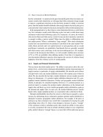
4.6.1.1 Decision Making under the HMT
Decision making when using the HMT can be represented by the algorithm
represented in figure 4.12.
We start with the narrowest product or geographic market definition which is

usually called the “focal product” and actually usually also the focal product of
the investigation. We then need to evaluate whether a monopolist of this product
could profitably raise prices by 5–10% for a year. If so, that single product will then
33
A nice treatment ofthe SSNIP test is provided in the paper by the previous chairman of the U.K. Com-
petition Commission, Professor Paul Geroski, and his coauthor, Professor Rachel Griffith (see Geroski
and Griffith 2003).
34
This “tradition” in the competition policy world is potentially a dangerous one in the sense that in
some markets a 5% price rise would correspond to an absolutely enormous increase in profitability. For
example, in markets where volumes are high and margins are thin (e.g., 1%), a 5% increase in prices
may correspond to a 500% increase in profitability. Relatedly, the consumer welfare losses associated
with a 5% increase in prices may in some circumstances (particularly in very large markets) be huge. In
such cases, it may be appropriate to worry about monopolization of markets even where monopolization
only leads to an ability to increase prices by say 1% or 2%. As always, the key is for the analyst to think
seriously about whether there are sufficient grounds for moving away from the normal practice of using
5–10% price increases for this exercise.
4.6. Measuring Pricing Constraints 203
Start with the narrowest product
or geographic market definition.
Is it profitable for a monopoly producer of
that product to increase prices in a small but
significant and nontransitory way (SSNIP)?
There must be at least one good substitute
excluded from the current market definition.
Expand the market to include it.
Now have a multiproduct monopolist.
Could he/she profitably raise prices?
Stop.
Market definition

is wide enough.
No
Yes
No
Yes
Figure 4.12. The HMT decision tree.
constitute our antitrust market. If not, we must include the “closest” substitute, that
product which provides the best alternative to consumers facing the price increase.
We then assume again a hypothetical monopolist, this time of each of the products
in our newly expanded set of products in our candidate market and we repeat our
question, will a 5–10% price increase for a year be profitable? This process continues
as long as the answer to the question is “no.” A “no” indicates that we are missing
at least one good substitute from our current candidate market definition and the
omitted product is constraining the profitability of raising prices for our monopolist.
We stop the process of adding products when we have a set of products that does
indeed allow the hypothetical monopolist to profitably raise prices without losing
customers to outside products. We define our antitrust market as the final set of
products, the set of products which it is “worth monopolizing.”
To illustrate further, suppose we face a situation in which three firms produce
three products called, somewhat uninspiringly, products 1, 2, and 3. Each of these
products is in fact a very good substitute; for the sake of argument, suppose they
are perfect substitutes. Suppose also that there are two other products, products 4
and 5, which are rather poorer substitutes. Product 1 is the focal product. Table 4.7
demonstrates the step-by-step application of the HMT to this case.
204 4. Market Definition
Table 4.7. Steps in a hypothetical monopolist test. PMD is proposed market definition.
Step 1 Step 2 Step 3
PMD f1gf1; 2gf1; 2; 3g
Q Does monopolization
of product 1 give

pricing power?
Does a (hypothetical)
monopolist of
products 1 and 2 have
pricing power?
Does a (hypothetical)
monopolist of products 1,
2, and 3 have pricing
power?
A No, because there
are two perfect
substitutes omitted
from the proposed
market. No ability
to raise price of
good 1.
No, because there is
still a perfect substitute
omitted from the
proposed market
(product 3) that
constrains the ability of
our hypothetical
monopolist of goods 1
and 2 to raise their
prices.
Yes, if products 4 and 5
are not good enough
substitutes. If so, then
the market definition of

f1; 2; 3g is accepted. No,
if either product 4 or 5 is
a good enough substitute
to constrain profitability
of price increase. In that
case, continue the test.
Suppose we did not use the HMT at step 3 but just looked at the pricing power
of three independent firms. Those firms would have no pricing power because of
constraints that come from within the proposed market definition. For example, the
firm producing 3 will have no market power because of the presence of producers of
goods 1 and 2. Thus the HMT works by explicitly putting the focus on the constraints
on pricing power that come from outside the proposed market definition.
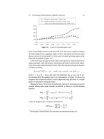
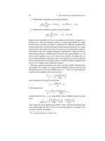
4.6.1.2 Implementation of the SSNIP Test
The SSNIP test consists of evaluating whether a 5–10% price increase for all the
products in the candidate market will produce a profit. Consider the single-product
candidate market. Recall that the firm’s profits are the total revenues minus the total
variable and fixed costs:
˘.p
t
/ D .p
t
 c/D.p
t
/  F;
where, for simplicity, we have assumed a constant marginal cost. The change in
profits due to an increase in prices from p
0
to p
1
can then be expressed as

˘.p
1
/  ˘.p
0
/ D .p
1
 p
0
/D.p
1
/  .p
0
 c/.D.p
0
/  D.p
1
//;
where the first term of the equality is the gain in revenues from the increase in prices
on the sales at p
1
and the second term is the loss of margins due to the decrease in
sales after the price hike. The core question is whether the drop in volume of sales at
the new price, and consequent loss in variable profit, is big enough to outweigh the
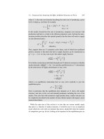
increased revenues obtained on goods still sold. This trade-off is shown graphically
in figure 4.13.
4.6. Measuring Pricing Constraints 205
P
1
P
0

D
c
Q
1
Q
0
Gained revenue from
higher price on
goods still sold
Lost margins on goods
no longer sold
+
−
Q
P
Figure 4.13. The trade-off when evaluating the profitability of a price increase.
Evidently, the crucial assumption of the SSNIP test is that the fall in demand will
be large when there are good substitutes available. In fact, we can show that it will
be profitable for the monopolist to raise its prices as long as its margin is lower than
the inverse of its own-price elasticity of demand.
In our benchmark model, a hypothetical monopolist of a single product in
a potentially differentiated product market will solve the profit-maximization
problem:
max
p
1
˘.p
1
Ip
2

;:::;p
J
/ D max
p
1
.p
1
 c/D.p
1
;p
2
;:::;p
J
/:
A monopolist of product 1 will increase price as long as it raises their profits, i.e.,
as long as
@˘.p
1
;p
2
;:::;p
J
/
@p
1
D .p
1
 c/
@D.p
1

;p
2
;:::;p
J
/
@p
1
C D.p
1
;p
2
;:::;p
J
/
> 0:
We can rearrange the expression to obtain
p
1
 c
p
1
6 
D.p
1
;p
2
;:::;p
J
/
p

1
Â
@D.p
1
;p
2
;:::;p
J
/
@p
1
Ã
1
D
1
Á
11
.p
1
;p
2
;:::;p
J
/
:
We will want to evaluate whether this inequality holds for all prices between p
Comp
1
and p
5%

1
D 1:05p
Comp
1
or p
10%
1
D 1:10p
Comp
1
respectively depending on whether we
use a 5% or 10% price increase. In this model, the data we need to perform the single-
product variant of the SSNIP test are therefore (i) the firms’ margin information
under competitive conditions and (ii) the product’s (candidate market’s) own-price
206 4. Market Definition
elasticity of demand (again in the range Œp
Comp
1
;p
5%
1
 or Œp
Comp
1
;p
10%
1
).
35
For imple-

mentation, the important aspect of this single-product variant of the test is that we do
not need a full set of cross-price elasticities of demand. The pricing theory analysis
of substitutability (usually associated with measuring cross-elasticities) turns into
a problem which only involves an evaluation of the own-price elasticity of demand
and a comparison of it with variable profit margins. (We will say more shortly.)
A common shortcut for the SSNIP test in geographical market definition is to
consider the cost of transporting goods from outside areas intothe candidate markets.
This relies on the assumption that goods are homogeneous and buyers are indifferent
as to the origin of the good. If transport costs are low enough that a price increase by
up to 10% by the hypothetical monopolist is likely to be met by an inflow of cheaper
product from elsewhere, the candidate market needs to be widened to include the area
where the shipped goods are coming from. Evidence on existing shipping activity
and transportation costs are therefore often used in practice to determine geographic
market definitions.
The purpose of the SSNIP test is to check whether the hypothetical monopolist
would find it profitable to increase prices from the competitive level by a material
amount (perhaps 5–10%) for a material amount of time (perhaps one year). Note that
the reference price for this evaluation is usually described as the “competitive price.”
This benchmark element of the test is crucial and sometimes it proves problematic
as we will illustrate in the next section.
In a formal application of SSNIP we may have an estimate of the marginal cost
and also an estimate of a demand curve. This in turn gives us a description of the
determinants of profitability so that we can directly evaluate whether
˘.1:05p
Comp
1
Ip
2
;:::;p
J

/  ˘.p
Comp
1
Ip
2
;:::;p
J
/
D .1:05p
Comp
1
 c/D.1:05p
Comp
1
;p
2
;:::;p
J
/
 .p
Comp
1
 c/D.p
Comp
1
;p
2
;:::;p
J
/

> 0:
At this point, we present a brief aside, aiming to note that there is a theoretical
underpinning to the observation that the own-price elasticity of demand is informa-
tive about substitution opportunities. In fact, we only need for income effects to be
small enough to interpret own-price elasticities as the substitution effect. In most
fast-moving consumer goods, the income effect will be relatively small, so when we
look at the own-price elasticity of demand we are mostly talking about the sum of all
the cross-price effects. Looking at own-price elasticity is appropriate when trying
to assess the constraint of substitutes as long as we can be confident, as is generally
the case, that the income effect is not playing a major role in the decision making.
35
It will often be very difficult to tell whether the own-price elasticity varies materially in the range,
and it is usual to only report a single number estimated using the predicted change in quantity following
a 5 or 10% change in prices. Such an elasticity estimated between two given points is also known as an
arc-elasticity.
4.6. Measuring Pricing Constraints 207
When a function is homogeneous of degree zero, as is the case for an individual’s
demand function for a product j , we can apply Euler’s theorem
36
J
X
kD1
p
k
@q
j
.p; y/
@p
k
C y

@q
j
.p; y/
@y
D 0:
We then obtain
1
q
j
.p; y/
Ä
@q
j
.p; y/
@ ln p
j
C
X
k¤j
@q
j
.p; y/
@ ln p
k
C
@q
j
.p; y/
@ ln y


D 0;
which in turn can be written as
Á
jj
C
X
k¤j
Á
jk
C Á
jy
D 0 or  Á
jj
D
X
k¤j
Á
jk
C Á
jy
:
This relationship suggests that the own-price elasticity of demand will be large when
either substitution effects are large or the income effect is large. The latter is caused
by the fact that the increase in price reduces the customer’s real income and their
income elasticity is high.
Finally, note that the homogeneity property relies on us doubling the prices of
all possible goods in the economy as well as income. In practice, we may treat
one good as a composite good consisting of “everything outside the set of goods
explicitly considered as potentially within the market,” or more simply the “outside
good.” There will often not be any price data for the outside good, although we

could use general price indices as an approximation. Substitution effects can occur
to the outside good, so that if we doubled all inside good prices and income we will
see that demand for the set of inside goods will fall. If so, then the own-price effects
will be larger in magnitude than the sum of the substitution effects (to inside good
products) plus the income effect.
More generally, of course, we will want to evaluate whether a price increase for a
collection of products is profitable.We discuss this case further in section 4.6.3. First,
we consider a particular type of difficulty that often arises—even in a single-product
context—when we apply the SSNIP test in practice.
4.6.1.3 The Cellophane and Reverse-Cellophane Fallacies and Other Difficulties
The Cellophane Fallacy. In the U.S. v. DuPont case in 1956
37
it was crucial to
determine whether cellophane (“plastic wrap”) represented a market. At that time
36
Assume a function homogeneous of degree r. By definition we have
q
j
.p
1
;p
2
;:::;p
J
;y/D 
r
q
j
.p
1

;p
2
;:::;p
J
;y/:
We obtain Euler’s results by differentiating both sides with respect to .
37
United States v. E. I. DuPont de Nemours & Co., 351 US 377 (1956).
208 4. Market Definition
DuPont sold 75% of all cellophane paper but only 20% of all “flexible packaging
material,” a potential alternative market definition. The U.S. Supreme Court ruled in
favor of DuPont accepting the appropriate market definition as “flexible packaging
material” and clearing the company of attempting to monopolize that market. The
reason was that at the prevailing price levels, the court found substantial evidence
of demand substitution between cellophane and other packaging materials, such as
greaseproof paper.
This case has given rise to the term “cellophane fallacy.” The idea is simple. If
the Court were looking at evidence from a market which was already monopolized,
then the price would already be raised to the point where a number of consumers
would already have looked around for imperfect substitutes and indeed switched to
them. Furthermore, the remaining customers may substitute away in large numbers
if prices were further increased by small amounts since monopolists will always
increase prices up to a level where their demand becomes elastic. As long as the
demand elasticity is below 1, it is profitable to raise prices and a monopolist would
already have done so. This provides a substantive difficulty when defining markets
in cartel, monopolization, and sector inquiries using evidence on observed levels
of substitution. We will find lots of substitution at monopoly prices and so we will
always find markets to be larger than we would if competitive prices were used as
the benchmark since prices will have been raised to the point where consumers are
considering switching (or quitting). Because this was not understood, the court may

have incorrectly determined that greaseproof paper constrained the pricing power
of DuPont when selling cellophane (plastic wrap).
The lesson is that it is crucial for the hypothetical monopoly test that we evaluate
the profitability of a price increase starting from competitive conditions, i.e., starting
with competitive prices and margins. The difficulty is that we may not know what
competitive conditions are—and assumptions about the competitive price level will
determine the answer for market definition. Specifically, if we determine that actual
prices are more than 5% above the unobserved competitive market prices, then we
will conclude that our market definition is sufficient and our player is a monopolist.
Unfortunately, such an approach would be entirely circular—our assumption would
determine our conclusion. There are no easy solutions to this difficulty, but we will
describe a range of tools to help determine when observed prices are competitive in
chapter 6.
The cellophane fallacy emerges as a central issue only infrequently in merger
cases, but nonetheless can arise in at least one guise. Specifically, if in truth the firms
are actually monopolists, but there is little substitutability between the products at
high prices, then in applying the SSNIP test we may begin the process of looking
for other relevant substitutes since raising prices beyond current (monopoly) levels
is evaluated to be unprofitable. Fortunately, we will not typically emerge from such
a process with a wrong decision even if we end up with a wider market since the
competitive effects analysis will usually generate a clearance result—that increasing
4.6. Measuring Pricing Constraints 209
prices further is unprofitable and hence the merger would be approved under a
standard evaluating whether a particular merger will “significantly impede effective
competition” (EC (Merger) Regulation no. 139/2004) or result in a “substantial
lessening of competition” test (the U.K. Enterprise Act 2003 or Section 7 of the
U.S. Clayton Act 1914).
38
The Reverse Cellophane Fallacy. Froeb and Werden (1992) point out that closely
related difficulties can arise when observed prices are below competitive prices. At

prices below competitive prices consumers may think the choice between two prod-
ucts is particularly obvious and we may observe little switching between products
in response to small variations in relative prices. If so, then we will conclude that
markets are narrowly drawn even if, in truth, pricing constraints are severe. Preda-
tory pricing investigations are the most obvious candidates for this difficulty, but it
can also arise as an issue in other contexts. For example, observed prices can be “too
low” when there are important “menu costs” faced by companies in changing their
prices. In the anticipated acquisition of Vernons by Sportech considered by the U.K.
Competition Commission in 2007, Sportech had last changed their price in 1999, at
which point they had increased their nominal prices by 25%.
39
The evidence sug-
gested that the reason for these infrequent but large price increases was that price
changes “disturbed” the customer base and led to consumers switching away from
playing the particular gambling product being sold (the football pools). If consumers
react to new information by making an explicit evaluation about whether to continue
with a particular activity (reoptimizing), whereas in the absence of change they will
continue playing, then, as with more traditional menu costs, it may be optimal for
the firm to introduce price changes in large discrete amounts infrequently rather
than small amounts frequently. The result may be that observed pries are below the
competitive level so that firms will appear to have a clear incentive to increase them.
The implication for market definition may be that markets are drawn too narrowly
in such situations.
The Counterfactual. In merger investigations the central question is often whether
the merger will result in an increased ability to raise prices. Often this means we can
38
Note that, more precisely, Section 7 of the Clayton Act 1914 describes that mergers and acquisitions
are prohibited where “the effect of such acquisition may be substantially to lessen competition, or tend
to create a monopoly.” In fact, one of the most important legal words in this sentence is “may,” which
has meant that the courts have decided that “Section 7 does not require proof that a merger or other

acquisition has caused higher prices in the affected market. All that is necessary is that the merger
create an appreciable danger of such consequence in the future. A predictive judgement, necessarily
probabilistic and judgmental rather than demonstrable, is called for.” Hospital Corp of America v. Federal
Trade Commission, 807 F. 2d 1281, 1389 (7th Cir. 1986). See also U.S. v. Philadelphia National Bank,
374 U.S. 321, 362 (1963). In Europe, Article 2(3) of Council Regulation (EC) no. 139/2004 provides
that the Commission must assess whether a merger or acquisition “would significantly impede effective
competition, in the common market or in a substantial part of it, in particular as a result of the creation
or strengthening of a dominant position.”
39
www.mmc.gov.uk/rep_pub/reports/2007/533sportech.htm. See the final report at paragraph 5.6.
210 4. Market Definition
use existing pre-merger prices even if some market power is being exercised, since
in many jurisdictions the statutory test is whether a merger substantially lessens
competition. There are, however, occasions where parties debate the right price to
use. For example, in the Sportech/Vernons merger inquiry the parties raised prices
by 25% during the inquiry (beginning the process of rolling out the price increases
in August 2007) and argued that the SSNIP test should be applied at the new higher
price level. Their reasoning was that the price increase was (i) proposed before
the acquisition and moreover (ii) was not in any event contingent on the merger
being approved. For each reason they argued the relevant benchmark from which
to perform the SSNIP test should involve prices after the 25% increase. The first
argument implies the relevant pre-merger price includes the 25% increase. The
second argument implies that competitive prices should be considered not as pre-
merger prices but rather as those prices that would prevail in the future, absent
the merger. Obviously, such arguments need to be treated with great caution by
competition authorities. In this case documentary evidence traced the proposal to
the price increase back to August 2006, but even this was not clearly before the
acquisition was under serious contemplation so that the evidence did not clearly
support this view. On the second point, in August 2007, Sportech actively began
rolling out the 25% price increase to their customers (who may sign up to play the

football pools once a week for say eight or ten weeks so that price increases bind
only on the renewal of a multiweek contract) potentially indicating that it would go
ahead irrespective of the merger. Even so, in this case, the CC did not consider this
evidence as entirely convincing as, for example, a price increase could be reversed
if the merger were in fact blocked.
To summarize, if competitive conditions are not observed, then competitive prices
and margins will sometimes need to be chosen or estimated. In cartel cases or
sector/market investigations a simple analysis which, for instance, considered that
competitive prices are 5% below the current level would automatically imply a
market definition (increasing prices by 5% would be profitable). In chapter 6, we
will consider how this problem can be addressed so that we can predict what prices
would look like under competition even if the data were generated under a monopoly.
Doing so will involve building a model either explicitly or implicitly of price-setting
behavior in the industry and in particular how it would change if we changed market
structure. Less formally, the tools we discuss in chapter 5 may well also be helpful
for this purpose.
4.6.2 Critical Loss Analysis
Critical loss analysis
40
is conceptually closely related to the hypothetical monopolist
test. It also uses information about demand and in particular the own-price elastic-
40
This section draws on Harris and Simons (1989) and also the working papers by O’Brien and
Wickelgren (2003) and by Katz and Shapiro (2003).
4.6. Measuring Pricing Constraints 211
ity of demand to make inferences about the price constraint exerted by substitute
products. The question asked in critical loss analysis is the following: How much
do sales need to drop in order to render an x% price increase unprofitable? In the
context of a benchmark homogeneous product model, this question is answered by
the following formula:

% Critical loss D 100 
%Prices
%Prices C % Initial margin
:
To derive this critical loss formula, one needs to calculate the demand after the price
increase D.p
1
/ such that given the original demand D.p
0
/, the original price p
0
,
and the higher price p
1
we have
˘.p
1
/  ˘.p
0
/ D .p
1
 p
0
/D.p
1
/  .p
0
 c/.D.p
0
/  D.p

1
// D 0:
Rearranging we obtain
.p
1
 p
0
/ŒD.p
1
/  D.p
0
/ C D.p
0
/  .p
0
 c/.D.p
0
/  D.p
1
// D 0;
.p
1
 p
0
C .p
0
 c//.D.p
1
/  D.p
0

// C D.p
0
/.p
1
 p
0
/ D 0;
D.p
1
/  D.p
0
/
D.p
0
/
D
p
1
 p
0
p
0
Â
p
1
 p
0
p
0
C

p
0
 c
p
0
Ã
:
This is equivalent to
% Critical loss D
100  %Prices
%Prices C % Initial margin
:
To illustrate the use of this formula, consider a 5% increase in prices in a market
where the margin at current prices is 60%:
% Critical loss D
100  %Prices
%Prices C % Initial margin
D
100  5%
5% C 60%
D 7:7%:
If the quantity demanded falls by more than 7.7% following the 5% price increase,
the price increase is not profitable and our candidate market must be expanded.
At least three issues commonly emerge in applying a critical loss test. First, the
fact that a 5% price increase is not profitable does not mean that a 50% price increase
is not profitable. Yet, we are interested in market power and would clearly wish to
draw narrow market boundaries if we found that a hypothetical monopolist could
raise prices by 50%.
Second, parties will often argue that the critical loss is likely to be far smaller
than the drop in sales that would actually be experienced by a 5% price increase

212 4. Market Definition
Table 4.8. Critical loss calculations for various margins using a 5% price increase.
Margin 40% 75% 90%
Critical loss 11.1% 6.3% 5.3%
and therefore a 5% price increase would be unprofitable. When accepting evidence
of actual sales declines following price increases, agencies need to be careful about
the potential endogeneity of price and sales changes.
Third, when considering critical loss calculations, it is very important to bear in
mind that if pre-merger margins are high, i.e., if .p
0
 c/=p
0
is big, each unit less
of sales is associated with a large fall in profits and so we will get a critical loss in
sales that is small. To illustrate, in the case of a 5% price increase we obtain the
values for the critical loss shown in table 4.8.
This issue is related to the cellophane fallacy because if the margin is high, it
means market power is probably already being exercised and so one must be careful
to rely on the effect of price changes on an already supra-competitive price level
when drawing conclusions about substitutability and market definition. If the firm
has market power, it will increase price up to the point where margins are high and
therefore the critical loss appears small.
The “fallacy” in this analysis is to treat the elasticity and the margin as if they
were independent from each other. In fact, according to the benchmark model,
margins tell us about the own-price elasticity before the price increase. If margins
are high, it implies a low price elasticity and that in turn suggests perhaps even
strongly there will be low actual losses due to a price increase. Firms sometimes
argue that because their critical loss is small, their actual loss is probably bigger and
the market should be large. Such arguments should not be accepted uncritically, but
rather parties should be pressed to explain why they would have a low elasticity of

demand evidenced by the high margins and relatively large actual losses of demand
following a price increase.
More generally, this is one example of a tension between the pieces of “data” (the
margin and the likely actual loss resulting from a price rise) and the model—which
states the Lerner index is inversely related to the own-price elasticity of demand.
Whenever a model and our pieces of data are difficult to reconcile, we will want
to question each. The apparent tensions may be reconciled by the finding that one
or more pieces of data are “wrong,” or alternatively that the data are right but the
benchmark model is not the correct one for this industry. It is very important to note
that the exact form of the critical loss formula depends explicitly on the monopoly
model being used to characterize the industry. Thus, table 4.8 captures the results
only of one particular type of critical loss exercise.
Finally, we note that itis possible, and sometimes appropriate, to undertake critical
loss analysis in terms of product characteristics other than price. For example, in
the Sportech/Vernons merger, Sportech’s advisors presented a critical loss analysis
4.6. Measuring Pricing Constraints 213
evaluating whether it would be profitable to reduce the quality of the gambling
product being sold, in particular the size of the jackpot paid out to the winner and,
relatedly, the fraction of the total “pool” of bets paid out as prizes.
41
4.6.3 SSNIP Test with Differentiated Products
The SSNIP test discussed above, as well as the critical loss analysis, was presented
for a single-product candidate market. In practice, we will often need to undertake,
formally or informally, a SSNIP test in a multiproduct context.
To do so we must make a number of decisions. For instance, we must consider
whether a hypothetical monopolist of our candidate collection of products has an
incentive to materially increase prices, and we usually assume we mean a 5% price
increase of all the prices within the candidate market. On the other hand, it may not
be appropriate to always increase all the product’s prices by 5% since the central ele-
ment of the SSNIP test is to consider whether material price increases are profitable

given a monopoly over a set of candidate products and it will not always, or even
usually in fact, be profit maximizing to apply an equal percentage price increase to
all products. A merger authority may decide that a material price increase is in fact
only 1% when investigating the impact of a particular inquiry or that price increases
may occur unevenly.
In a multiproduct context, the simplest approach is to assume that all goods inside
the market are effectively perfect substitutes. In that case, there is just one relevant
price so that the SSNIP test boils down to evaluating whether or not the candi-
date market’s own-price elasticity is sufficiently high to render a 5% price increase
unprofitable. For example, when considering whether the right market for eggs is
“free-range” or should be expanded to include “organic,” a reasonable approach is to
examine the own-price elasticity of (candidate market) demand faced by a hypothet-
ical monopolist for free-range eggs. Doing so would of course be far simpler than
worrying about a monopoly price for all the many different variants of free-range
eggs, even though there is in fact some modest amount of branding of eggs. If such
an approximation is not appropriate in the context being investigated, then SSNIP
can be applied more formally in a variety of ways.
Denoting the candidate market demand elasticity as Á
M
1
.p
1
Ip
2
;:::;p
J
/ we
evaluate whether
p
1

 c
p
1
6
1
Á
M
1
.p
1
;p
2
;:::;p
J
/
in the range between p
Comp
1
and p
5%
1
D 1:05p
Comp
1
(or, in practice, usually just at
p
5%
1
) holding the prices of all products outside the candidate market .p
2

;:::;p
J
/
41
See the U.K. Competition Commission’s report Sportech/Vernons (2007) and in particular Appen-
dix F to the final report, paragraphs 32–38 and Annex 1, where the analogous formulas are derived, given
a set of assumptions about the ways in which jackpots were related to profits. The report is available at
www.competition-commission.org.uk/rep
pub/reports/2007/fulltext/533af.pdf.
214 4. Market Definition
as fixed:
p
1
 c
p
1
6
1
Á
M
1
.p
1
;p
2
;:::;p
J
/
:
As always, if the elasticity is very low, there will be an incentive to increase prices. In

such a case, our approximationassumes that products within the candidate marketare
homogeneous so that there is a single price and candidate market demand function
and corresponding elasticity so that
Á
M
1
.p
1
;p
2
;:::;p
J
/ D
@ ln D
M
1
.p
1
;p
2
;:::;p
J
/
@ ln p
1
:
In fact, many markets will include differentiated products and given enough data
we will perhaps be able to pay attention (formally or informally) to the pattern of
substitution within the candidate group of products when determining whether a
general price increase for the group is profitable for the hypothetical monopolist.

A formal approach to this problem in a multiproduct context involves more data
and takes us some way toward a full merger simulation model. We will show that
for market definition purposes we will not normally need to undertake a full merger
simulation, but even so it is very useful to understand the deep interconnections
between the SSNIP test in a multiproduct context and a full merger simulation
model. Merger simulation is a large topic in itself and we discuss it extensively in
chapter 8 while this section provides an introduction to that chapter. In section 4.6.4
we outline the full equilibrium relevant market test (FERM) proposed in the 1984
U.S. guidelines and recently implemented by Ivaldi and Lorincz (2009), which is
far closer to undertaking a full merger simulation exercise and then “backing out” a
market definition. Finally, in section 4.6.5 we discuss the use of “residual” demand
functions (following Baker and Bresnahan (1985, 1988)) for market definition in
multiproduct contexts.
4.6.3.1 Multiproduct Profit Maximization
Consider a candidate market has been proposed which includes several differentiated
products. We will consider whether a hypothetical monopolist will have an incentive
to increase the prices of all products in the defined market. To begin with we consider
the candidate market consisting of the two products and look at the profitability of
a price increase in one of the products. We assume our hypothetical monopolist
chooses prices to maximize profits holding fixed the prices of those goods outside
the candidate market:
max
.p
1
;p
2
/
˘.p
1
;p

2
Ip
3
;:::;p
J
/;
where
˘.p
1
;p
2
Ip
3
;:::;p
J
/
D .p
1
 c
1
/D
1
.p
1
;p
2
;p
3
;:::;p
J

/
C .p
2
 c
2
/D
2
.p
1
;p
2
;p
3
;:::;p
J
/:
4.6. Measuring Pricing Constraints 215
The hypothetical monopolist will find increasing the price of good 1 profitable
whenever
@˘.p
1
;p
2
Ip
3
;:::;p
J
/
@p
1

> 0;
i.e.,
.p
1
 c
1
/
@D
1
.p
1
;p
2
;:::;p
J
/
@p
1
C D
1
.p
1
;p
2
;:::;p
J
/
C .p
2
 c

2
/
@D
2
.p
1
;p
2
;:::;p
J
/
@p
1
> 0:
The last term of the inequality represents the reinforcing effect of the increase of
the price p
1
on the demand for good 2. While independent producers of products 1
and 2 would ignore these cross-product effects, a multiproduct firm (or here our
hypothetical monopolist) would recognize the loss of sales of product 1, but treat
those customers that depart completely rather differently from those who were only
lost to product 2. In particular, she would take into account the revenue that arises
from consumers switching from good 1 to become purchasers of good 2. If goods
1 and 2 are substitutes, the derivative in this last term is positive. For that reason,
our hypothetical monopolist will want to increase price p
1
compared with the price
that would be set by a firm who only owned product 1.
If goods 1 and 2 are demand substitutes, a hypothetical monopolist will also have
an incentive to increase p

2
when p
1
increases.
In chapter 1 we established the general result that the slope of a firm’s reaction func-
tion (i.e., the profit-maximizing choice of action given the action(s) of rival firm(s))
depends on the sign of the cross-partial derivative of the firm’s profit function. For-
mally, that means the profit-maximizing choice of p
2
will increase as p
1
increases
if
@
2
˘.p
1
;p
2
Ip
3
;:::;p
J
/
@p
2
@p
1
D
@

@p
2
Â
@˘.p
1
;p
2
Ip
3
;:::;p
J
/
@p
1
Ã
> 0:
This in turn will give a boost to the profitability of increasing p
1
if
@
2
˘.p
1
;p
2
Ip
3
;:::;p
J
/

@p
1
@p
2
D
@
@p
1
Â
@˘.p
1
;p
2
Ip
3
;:::;p
J
/
@p
2
Ã
> 0:
Since the cross derivatives do notdependon the order of differentiation, either both of
these derivatives will be positive or neither will be. We showed that in differentiated
product pricing games, these cross derivatives depended crucially on whether goods
were substitutes or complements. Specifically, when goods 1 and 2 are substitutes,
a price increase of good 1 will result in firm 2 having an incentive to increase the
price of good 2 and this in turn will generate an incentive for a further price increase
for 1. These mutually reinforcing effects continue but in ever smaller amounts until
we find the new higher prices for both goods.

216 4. Market Definition
In practice, assessing the profitability of an increase in the price of each of the
products in the market will require information on the own-price elasticity, the
diversion ratios (DRs), relative prices, and the margins on both products. In fact, the
first-order conditions for profit maximization suggest that increasing prices will be
profitable if
p
1
 c
1
p
1
6
1
Á
11
.p
1
;p
2
;:::;p
J
/
C
p
2
 c
2
p
1

DR
12
and analogously the price increase for product 2 will be profitable if
p
2
 c
2
p
2
6
1
Á
22
.p
1
;p
2
;:::;p
J
/
C
p
2
 c
2
p
1
DR
21
:

Merger guidance in most jurisdictions suggests it will often be appropriate to apply
these formulas using the prices
p
1
D p
5%
1
Á 1:05p
Comp
1
and p
2
D p
5%
2
Á 1:05p
Comp
2
in order to examine whether it is profitable to increase p
1
and p
2
by 5% above
the competitive levels (or more precisely, since these are first-order conditions, to
evaluate whether it is profitable to undertake a further (tiny) price increase when
prices are 5% above the competitive level). Note that terms like .p
2
 c
2
/=p

1
can
be written as the product of a margin times relative prices,
p
2
 c
2
p
1
D
p
2
 c
2
p
2
p
2
p
1
:
For completeness we note that above formula is derived as follows. Denote p D
.p
1
;:::;p
J
/, then the first-order condition for profit maximization when setting the
price of good 1 states that p
1
should be increased when

.p
1
 c
1
/
@D
1
.p/
@p
1
C D
1
.p/ C .p
2
 c
2
/
@D
2
.p/
@p
1
> 0:
Rearranging:
.p
1
 c
1
/ C
D

1
.p/
@D
1
.p/=@p
1
C .p
2
 c
2
/
@D
2
.p/=@p
1
@D
1
.p/=@p
1
6 0;
where the inequality changes direction because
@D
1
.p/
@p
1
<0:
Dividing through by p
1
and using the definition of the diversion ratio gives

p
1
 c
1
p
1
C
1
@ ln D
1
.p/=@ ln p
1

p
2
 c
2
p
1
DR
12
6 0;
where the analogous formula can easily be written down for good 2.
4.6. Measuring Pricing Constraints 217
Table 4.9. Example calculation for multiproduct application of the SSNIP test.
Product 1 Product 2
Margin 10% 20%
Diversion ratio 0.29 0.5
|Own-price elasticity of demand| 2 4
Ratio of prices p

2
=p
1
11
Profitability calculation:
p
1
 c
1
p1
‹
6
1
Á
11
.p
1
;p
2
;:::;p
J
/
C
p
2
 c
2
p
2
p

2
p
1
DR
12
; 0:1 6
1
2
C 0:2  1  0:29 D 0:56
p
2
 c
2
p1
‹
6
1
Á
22
.p
1
;p
2
;:::;p
J
/
C
p
1
 c

1
p
1
p
1
p
2
DR
21
; 0:2 6
1
4
C 0:1  1  0:5 D 0:30
Note that this test in a two-product candidate market requires estimates of margins,
price elasticities and diversion ratios. While precise estimates of such information
are always difficult to obtain, it is not always impossible—so that this formula can
actively be applied in practical settings in order to help understand the incentives of
multiproduct hypothetical monopolists. An example of such application is given in
table 4.9.
4.6.3.2 Implementation of the Test with More than Two Products
(Merger Simulation)
The SSNIP can formally be applied in a general multiproduct context.
42
To do so,
we wish to evaluate whether monopolistic profits could be derived from goods in a
candidate market by a hypothetical monopolist. That is, we must effectively attempt
to evaluate profitability under competitive prices and then compare it with the profits
that would be generated if prices of all goods in the inside markets were increased
by a SSNIP amount, which generally means between 5 and 10% for a period of
about a year. If the price increase is profitable, the candidate market is declared a

relevant competition policy market.
Formally, suppose we define . Np
1
;:::; Np
M
/ are the competitive prices of goods in
a candidate market, consisting of the set of products, =
M
. A SSNIP test considers
whether a price increase to 1 C Ä/ Np
1
;:::;.1CÄ/ Np
M
/, where .1 CÄ/ D 1:05 or
1.10 would be profitable for a hypothetical monopolist of those goods. Given the
42
This section draws upon the mathematical formalization of the SSNIP test presented in Ivaldi and
Lorincz (2005). A modified version of the paper is found in Ivaldi and Lorincz (2009). We discuss this
interesting paper further in a section below. For now we note that not all practitioners would agree
that this definition is the right definition of a SSNIP test. For example, as we discuss below, in some
circumstances it may be appropriate to allow price increases which are not uniformly all 5% above the
competitive price.
218 4. Market Definition
profit function for the hypothetical monopolist of that set of products,
. Np
1
;:::; Np
J
/ D
X

j 2=
J
. Np
j
 c/D. Np
1
;:::; Np
M
;:::; Np
J
/;
it is easy to evaluate whether the change in prices is profitable by asking whether
 D  1 C Ä/ Np
1
;:::;.1C Ä/ Np
M
; Np
M C1
;:::; Np
J
/  . Np
1
;:::; Np
J
/
> 0:
The SSNIP market will be the smallest set of products, =
M
, such that a price increase
is profitable.

Analytically, we can evaluate whether the directional derivative is positive, i.e.,
whether
@ 1 C Ä/ Np
1
;:::;.1C Ä/ Np
M
; Np
M C1
;:::; Np
J
/
@Ä
> 0:
Implementing the hypothetical monopolist test with multiple products involves hav-
ing knowledge of pre-merger marginal costs and prices of goods inside and outside
the hypothetical monopoly. This exercise can be undertaken using merger simulation
models, which will be discussed in chapter 8. A nice example of the kinds of issues
which emerge when doing so is provided by Brenkers and Verboven (2005). In that
paper, the authors used a multiple-product SSNIP test to define market in the retail
automobile industry. They find that the markets that are defined using the SSNIP
test do not correspond to those described by the Standard Industry Classification
(SIC).
The SSNIP test assumes that the prices of the goods outside of the hypotheti-
cal monopoly stay constant following the price increase. In fact, if the goods are
related they are likely to react to the change in prices. The next section examines
the implications of relaxing this assumption.
4.6.4 The Full Equilibrium Relevant Market Test
The full equilibrium relevant market test (FERM), as proposed by the 1984 U.S.
Horizontal Merger Guidelines, is an alternative implementation of the hypotheti-
cal monopolist test (HMT) to the traditional SSNIP test. The idea is based on the

observation that the SSNIP test is not an equilibrium test in the sense that it does
not compare two situations in equilibrium and therefore it does not compare two
situations that would actually be found in the real world. To see why, note that the
SSNIP test supposes that a monopolist of a candidate market considers the prof-
itability of a unilateral price increase assuming no reaction to the price increase by
producers of goods outside the candidate market. In contrast, the FERM allows the
goods outside the candidate market to respond by changing their prices so we move
4.6. Measuring Pricing Constraints 219
to a new “equilibrium” set of prices for all products being sold, but where prices
inside the candidate market are set by the hypothetical monopolist.
43
Under FERM there will be a tendency to get narrower markets than under SSNIP
because price increases by the hypothetical monopolist will generally be followed
by price increases of substitutes outside the candidate market. These in turn will
tend to reinforce the profitability of the initial price increase and hence push us
toward narrower market definitions. Notice that the question of whether to hold
fixed competitive variables, such as price or quantity of those goods which are
outside the candidate market, is related to the question of whether to account for
supply substitution in market definition. When considering the constraint imposed
by supply substitution parties often argue that expansion of output by firms outside
the candidate market will defeat an attempted price increase. Parties argue that
the implication is that the market definition should be expanded to include other
products. In contrast, in a pricing game reactions by firms outside the market will
tend to reinforce price increases by the hypothetical monopolist because firms tend
to react to price increases by increasing their own prices, i.e., by restricting their
supply.
The example below from Ivaldi and Lorincz (2009) illustrates the effect of allow-
ing producers inside and outside the candidate market definition to react to a price
increase by the hypothetical monopolist consisting of all products sold inside the
candidate market using data from the market for computer servers. The mechanics

of applying the test are identical to the tools used in merger simulation, a topic
we discuss extensively in chapter 8. Consequently, here, we restrict ourselves to
reporting Ivaldi and Lorincz’s results.
Table 4.10 reports the results from applying the traditional SSNIP test to a model
estimated using data on computer servers from Europe. It applies the test using a 10%
price increase. Under the SSNIP test, a market for computer servers in the range of
€0–€2,000 is rejected because an attempt to increase prices by 10% in that segment
alone is estimated to be unprofitable. On the other hand, the SSNIP applied to all
servers priced between €0 and €4,000 does find it profitable to increase all prices
by 10%. Hence the SSNIP test suggests that there is a competition policy market for
relatively low-end computers, specifically the set of servers priced between €0 and
€4,000. In addition the results alsosuggest there is a mid-range market for computers
between €4,000 and €10,000 servers and a high-end market for computers above
€10,000.
Table 4.11 reports the analogous results applying the FERM test for market def-
inition. In doing so, Ivaldi and Lorincz obtain the same results for the competition
policy market definition for low-end computer servers but the mid range market is
43
For a detailed description of this method, see Ivaldi and Lorincz (2005) and the revised version Ivaldi
and Lorincz (2009). The former paper introduces the nicely descriptive name FERM. The latter drops
that name in favor of US84. We adopt the more descriptive term FERM.
220 4. Market Definition
Table 4.10. SSNIP test in the market for servers.
Lower price Upper price Number of % Change in
limit ($) limit ($) products profits (
SSNIP
M
)
0 2,000 27 1.2
0 3,000 55 1.5

0 4,000 123 1.7
4,000 5,000 58 5.6
4,000 6,000 112 2.1
4,000 7,000 134 2.0
4,000 8,000 166 1.2
4,000 9,000 191 0.3
4,000 10,000 229 2.6
10,000 12,000 21 24.7
:
:
:
:
:
:
:
:
:
:
:
:
10,000 1,000,000 272 10.1
Source: Ivaldi and Lorincz (2009).
split in two. Specifically they obtain one market for the €4,000–€6,000 range and
one for the €6,000–€10,000 range.
In a conventional application of the SSNIP test all prices are increased propor-
tionately. In contrast in a FERM test the hypothetical monopolist sets prices of the
subset of goods in the candidate market to maximize profits. That means that all
prices may increase by differing amounts. The SSNIP test may be applied similarly,
but alternatively, to address this concern, the authors propose basing their market
definition choice on the average percentage change in prices within the candidate set

of products when that set of products switches from competitive (initial equilibrium)
to the partially collusive equilibrium in which all prices are reset by the hypothetical
monopolist. Their application of the test then defines the set of products as being a
market when the average percentage change in prices is above 10%.
4.6.5 The Residual Demand Function Approach (To Market Power)
A related approach is that proposed by Scheffman and Spiller (1987) for homoge-
neous product markets and Baker and Bresnahan (1985, 1988) for differentiated
product markets. The approach is known as the residual demand function approach
and can be useful for evaluating the extent of market power or market definition
in some particular circumstances. However, these models are explicitly not imple-
menting a standard SSNIP test so that the results need not correspond to conclusions
that would be drawn from SSNIP tests even if the assumptions on which they rely
are correct. On the other hand, since these methods can be useful for evaluating
4.6. Measuring Pricing Constraints 221
Table 4.11. FERM test in the market of servers.
Lower price Upper price Number of % Average price
limit ($) limit ($) products change (p
M
)
0 2,000 27 4.3
0 3,000 55 7.6
0 4,000 123 2.1
4,000 5,000 58 5.1
4,000 6,000 112 11.0
6,000 7,000 22 0.2
:
:
:
:
:

:
:
:
:
:
:
:
6,000 300,000 357 9.8
6,000 400,000 365 10.4
400,000 500,000 9 0.004
:
:
:
:
:
:
:
:
:
:
:
:
400,000 1,000,000 24 0.2
Source: Ivaldi and Lorincz (2009).
the market power of firms, the residual demand approach can be used for market
definition in a fashion not unrelated to the FERM test. To see why, we first recall
the notion of a residual demand curve.
First, following Landes and Posner (1981) and Scheffman and Spiller (1987)
consider the dominant-firm model. In that model, the dominant firm faced a mar-
ket demand D

Market
.p/ and also a competitive fringe, acting as price-takers, who
are willing to supply an amount based on the price being offered in the market,
S
Fringe
.p/. The residual demand is then that which is left to the dominant firm after
the fringe has supplied any units they are willing to supply at that price,
D
Dominant
.p/ D D
Market
.p/  S
Fringe
.p/:
We showed in chapter 1, that the dominant firm’s price elasticity of demand is
Á
Dominant
Demand
D
1
Share
Dom
.Á
Market
Demand
 Share
Fringe
 Á
Fringe
Supply

/:
This is the residual elasticity of demand, which begins with the market elasticity
of demand and then adjusts it to take into account any supply adjustment from the
competitive fringe. Note that the residual elasticity of demand typically increases
in magnitude with the elasticity of market demand since Á
Market
Demand
<0and also
the elasticity of supply from the fringe since Á
Fringe
Supply
>0.
44
Having subsumed the
44
Note that when examining residual demand in this way we are incorporating supply substitution
from the fringe into our analysis.
222 4. Market Definition
supply response of the competitive fringe into a careful definition of the firm’s
demand function (as distinct from the market demand function), we can then use
our standard monopoly pricing formula to conclude that a dominant firm would want
to raise price so long as her margins are smaller than the inverse of the elasticity of
this “residual” demand elasticity.
The insight of the residual demand function approach is that the residual demand
function captures all of the relevant information about the constraint implied by
other firms and expresses it in terms of the residual demand elasticity. Specifically,
in considering the profitability of price rises for any firm (which for this example
and without loss of generality we shall call firm 1) we can substitute the prices
.p
2

;:::;p
J
/ with their equilibrium formula so that the calculation is effectively
about the partial residual demand curve elasticity. Firm 1 has an ability to raise
prices as long as
p
1
 mc
1
p
1
6
1
Á
Resid
11
:
Notice this is a starkly different calculation from using the SSNIP test for a single-
product candidate market definition which would evaluate the candidate market of
a single product by considering instead whether
p
1
 mc
1
p
1
6
1
Á
11

holding the prices of other goods fixed. For a derivation of the residual elasticity
and a more technical presentation, see section 4.6.6 below.
Such an analysis clearly provides us with information regarding the actual mar-
ket power of our dominant firm and, in particular, would suggest that those dom-
inant firms facing a competitive fringe with a high supply elasticity are unlikely
to have much pricing power. On the other hand, this analysis does not apply a
SSNIP to any candidate market (or at least not one as conventionally applied).
To see why, note that a SSNIP applied to the candidate market, “the dominant
firm,” would ordinarily hold constant the price being charged by rival suppliers,
whereas by definition here we have assumed a single price to derive the domi-
nant firm’s demand curve and in particular we have assumed that if the dominant
firm raises its price, then the competitive suppliers also face a raised price so that
the prices of firms “outside” the candidate market (dominant firm) are not held
fixed. Similarly, the analysis does not correspond to a SSNIP test on the candidate
market consisting of the dominant firm plus the competitive fringe since in that
case we would use the (market) demand curve, D
Market
.p/. On the other hand, the
approach is far closer to that suggested by the authors of the FERM approach to
market definition. That approach explicitly takes into account reactions by com-
petitors outside the candidate market. One could use the residual demand curve
approach for market definition testing a candidate market consisting of a domi-
nant firm alone against the alternative hypothesis of the dominant firm plus the