Geoscience and Remote Sensing, New Achievements Part 10 pot
Bạn đang xem bản rút gọn của tài liệu. Xem và tải ngay bản đầy đủ của tài liệu tại đây (2.24 MB, 35 trang )
GeoscienceandRemoteSensing,NewAchievements308
A.2 Discretization
Next, concerning the implementation and in order to describe the upward and downward
diffuses radiance hemispherical distribution, Verhoef (1998) proposes a discretization of hemi-
spheres: zenithal and azimuthal angles into N segments. In this case, L
−
and L
+
are replaced
by sub-fluxes defined over the hemisphere segments forming together vectors called E
−
and
E
+
, respectively. The operators of Eq. (72) are discretized accordingly, in particular, s, s
become vectors called s and s
, respectively, A, B becomes square matrices called A and B,
respectively, and v and v
become vectors called v and v
, respectively. Eqs. (72) (73) (74) (75)
(76) become (Verhoef, 1998):
d
dz
E
s
E
−
E
+
E
+
o
E
−
o
=
k 0 0 0 0
−s
A −B 0 0
s B
−A 0 0
w v v
−K 0
−w
−v
−v 0 K
E
s
E
−
E
+
E
+
o
E
−
o
, (85)
Note that, as in the continuous case [cf. Eq. (80)], A could be written as
A
= κ
κ
κ − B
. (86)
with κ
κ
κ and B
the discrete scattering matrices corresponding to k and B
, respectively.
The final solution linking the layer output fluxes to the input ones is (Verhoef, 1998)
E
s
(L)
E
−
(L)
E
+
(t)
E
+
o
(t)
E
−
o
(L)
=
τ
ss
0 0 0 0
τ
τ
τ
sd
T R 0 0
ρ
ρ
ρ
sd
R T 0 0
ρ
so
ρ
ρ
ρ
T
do
τ
τ
τ
T
do
τ
oo
0
τ
so
τ
τ
τ
T
do
ρ
ρ
ρ
T
do
0 τ
oo
E
s
(t)
E
−
(t)
E
+
(L)
E
+
o
(t)
E
−
o
(L)
, (87)
where
(L) and (t) refer to the bottom and top of the layer, respectively.
Now, let us consider the case when the source changes. This change includes both the direc-
tion and the way that the direct flux is scattered under the vegetation. Since the scattering
properties depend only on the vegetation parameters and the source solid angle, the latter
possibility of change does not have a physical meaning. However, it is needed in our case
to define the scattering parameter when an effective vegetation density is considered. The
variation has an impact over the scattering parameters of Eq. (85) as follows. The terms k,
s
, s and w change and the other matrix terms remain constant. The consequences over the
boundary condition matrix concern elements that depend on the source, and are: τ
ss
, τ
τ
τ
sd
, ρ
ρ
ρ
sd
,
ρ
so
and τ
so
. Thus, to allow their estimation, an explicit dependency of the boundary terms on
the scattering ones has to be accomplished:
{τ
ss
⇒ τ
ss
(k),τ
τ
τ
sd
⇒ τ
τ
τ
sd
(k,s
,s),ρ
ρ
ρ
sd
⇒ ρ
ρ
ρ
sd
(k,s
,s),ρ
so
⇒ ρ
so
(k,s
,s, w),τ
so
⇒ τ
so
(k,s
,s,w
)}.
(88)
Moreover, in the discrete leaf case, the hot spot effect is taken into account in the computation
of ρ
so
, in this case it will be noted as ρ
HS
so
(Verhoef, 1998).
To distinguish SAIL++ boundary matrix terms from our model terms,
++ will be added to
SAIL++ terms as upperscript.
A.3 SAIL++ equation reformulation
In our study, we need to separate the upward diffuse fluxes created by the first collision with
leaves of direct flux from the upward fluxes created by multiple collisions, the corresponding
radiances are called L
1
+
and L
∞
+
, respectively. Indeed, a specific processing for L
1
+
is proposed
in this paper in order to take into account the hot spot effect as well as to conserve energy.
As defined, L
1
+
depends on E
s
and can be extended when traveling under the vegetation.
Compared to L
+
[cf. Eq. (74)], L
1
+
does not increases by L
−
and L
1
+
itself scattering. Thus its
variation is governed by [cf. Eq. (80)]
dL
1
+
(z,Ω
+
)
dz
= [s ◦ E
s
(z,Ω
s
)](Ω
+
) −[k ◦ L
1
+
(z)](Ω
+
). (89)
Now, concerning L
∞
+
, it does not depend any more on E
s
. However it increases by L
1
+
, L
−
and
L
∞
+
itself scattering and decreases, as usual, by extinction. It is given by
dL
∞
+
(z,Ω
+
)
dz
= [B
◦ L
1
+
(z)](Ω
+
) + [B ◦ L
−
(z)](Ω
+
) −[A ◦ L
∞
+
(z)](Ω
+
), (90)
According to this decomposition, the reformulation of SAIL++ equation set is as follows. Eq.
(74) has to be replaced by Eqs. (89) and (90). In Eqs (73), (75) and (76), L
+
has to be replaced
by L
1
+
+ L
∞
+
. One obtains
dL
−
(z,Ω
−
)
dz
= −[s
◦E
s
(z,Ω
s
)](Ω
−
) + [A ◦L
−
(z)](Ω
−
) −[B ◦L
1
+
(z)](Ω
−
) −[B ◦L
∞
+
(z)](Ω
−
),
(91)
dE
+
o
(z,Ω
o
)
dz
= wE
s
(z,Ω
s
) + [v ◦ L
−
(z)] + [v
◦ L
1
+
(z)] + [v
◦ L
∞
+
(z)] − KE
+
o
(z,Ω
o
), (92)
dE
−
o
(z,Ω
o
)
dz
= −w
E
s
(z,Ω
s
) −[v
◦ L
−
(z)] − [v ◦ L
1
+
(z)] − [v ◦ L
∞
+
(z)] + KE
−
o
(z,Ω
o
). (93)
The reformulated SAIL++ equation set is composed by Eqs. (72), (91), (89), (90) (92) and (93).
B. Vegetation local density
To define a realization of a vegetation distribution within the canopy in the discrete leaf case,
Knyazikhin et al. (1998) propose the definition of an indicator function:
χ
(
r) =
1, if
r ∈ vegetation,
0, otherwise,
(94)
where
r = (x,y,z) is a point within the canopy. Then, they define a fine spatial mesh by
dividing the layer into non-overlapping fine cells
(e(
r)) with volume V[e(
r)]. Thus, the foliage
area volume density (FAVD) could be defined as follows:
u
L
(
r) =
1
V
[e(
r)]
t∈e(
r)
χ(
t)d
t. (95)
By defining the average density of leaf area per unit volume, called d
L
(depends only on leaf
shape and orientation distribution), u
L
is written simply as follows
u
L
(
r) = d
L
χ(
r). (96)
OpticalandInfraredModeling 309
A.2 Discretization
Next, concerning the implementation and in order to describe the upward and downward
diffuses radiance hemispherical distribution, Verhoef (1998) proposes a discretization of hemi-
spheres: zenithal and azimuthal angles into N segments. In this case, L
−
and L
+
are replaced
by sub-fluxes defined over the hemisphere segments forming together vectors called E
−
and
E
+
, respectively. The operators of Eq. (72) are discretized accordingly, in particular, s, s
become vectors called s and s
, respectively, A, B becomes square matrices called A and B,
respectively, and v and v
become vectors called v and v
, respectively. Eqs. (72) (73) (74) (75)
(76) become (Verhoef, 1998):
d
dz
E
s
E
−
E
+
E
+
o
E
−
o
=
k 0 0 0 0
−s
A −B 0 0
s B
−A 0 0
w v v
−K 0
−w
−v
−v 0 K
E
s
E
−
E
+
E
+
o
E
−
o
, (85)
Note that, as in the continuous case [cf. Eq. (80)], A could be written as
A
= κ
κ
κ − B
. (86)
with κ
κ
κ and B
the discrete scattering matrices corresponding to k and B
, respectively.
The final solution linking the layer output fluxes to the input ones is (Verhoef, 1998)
E
s
(L)
E
−
(L)
E
+
(t)
E
+
o
(t)
E
−
o
(L)
=
τ
ss
0 0 0 0
τ
τ
τ
sd
T R 0 0
ρ
ρ
ρ
sd
R T 0 0
ρ
so
ρ
ρ
ρ
T
do
τ
τ
τ
T
do
τ
oo
0
τ
so
τ
τ
τ
T
do
ρ
ρ
ρ
T
do
0 τ
oo
E
s
(t)
E
−
(t)
E
+
(L)
E
+
o
(t)
E
−
o
(L)
, (87)
where
(L) and (t) refer to the bottom and top of the layer, respectively.
Now, let us consider the case when the source changes. This change includes both the direc-
tion and the way that the direct flux is scattered under the vegetation. Since the scattering
properties depend only on the vegetation parameters and the source solid angle, the latter
possibility of change does not have a physical meaning. However, it is needed in our case
to define the scattering parameter when an effective vegetation density is considered. The
variation has an impact over the scattering parameters of Eq. (85) as follows. The terms k ,
s
, s and w change and the other matrix terms remain constant. The consequences over the
boundary condition matrix concern elements that depend on the source, and are: τ
ss
, τ
τ
τ
sd
, ρ
ρ
ρ
sd
,
ρ
so
and τ
so
. Thus, to allow their estimation, an explicit dependency of the boundary terms on
the scattering ones has to be accomplished:
{τ
ss
⇒ τ
ss
(k),τ
τ
τ
sd
⇒ τ
τ
τ
sd
(k,s
,s),ρ
ρ
ρ
sd
⇒ ρ
ρ
ρ
sd
(k,s
,s),ρ
so
⇒ ρ
so
(k,s
,s, w),τ
so
⇒ τ
so
(k,s
,s,w
)}.
(88)
Moreover, in the discrete leaf case, the hot spot effect is taken into account in the computation
of ρ
so
, in this case it will be noted as ρ
HS
so
(Verhoef, 1998).
To distinguish SAIL++ boundary matrix terms from our model terms,
++ will be added to
SAIL++ terms as upperscript.
A.3 SAIL++ equation reformulation
In our study, we need to separate the upward diffuse fluxes created by the first collision with
leaves of direct flux from the upward fluxes created by multiple collisions, the corresponding
radiances are called L
1
+
and L
∞
+
, respectively. Indeed, a specific processing for L
1
+
is proposed
in this paper in order to take into account the hot spot effect as well as to conserve energy.
As defined, L
1
+
depends on E
s
and can be extended when traveling under the vegetation.
Compared to L
+
[cf. Eq. (74)], L
1
+
does not increases by L
−
and L
1
+
itself scattering. Thus its
variation is governed by [cf. Eq. (80)]
dL
1
+
(z,Ω
+
)
dz
= [s ◦ E
s
(z,Ω
s
)](Ω
+
) −[k ◦ L
1
+
(z)](Ω
+
). (89)
Now, concerning L
∞
+
, it does not depend any more on E
s
. However it increases by L
1
+
, L
−
and
L
∞
+
itself scattering and decreases, as usual, by extinction. It is given by
dL
∞
+
(z,Ω
+
)
dz
= [B
◦ L
1
+
(z)](Ω
+
) + [B ◦ L
−
(z)](Ω
+
) −[A ◦ L
∞
+
(z)](Ω
+
), (90)
According to this decomposition, the reformulation of SAIL++ equation set is as follows. Eq.
(74) has to be replaced by Eqs. (89) and (90). In Eqs (73), (75) and (76), L
+
has to be replaced
by L
1
+
+ L
∞
+
. One obtains
dL
−
(z,Ω
−
)
dz
= −[s
◦E
s
(z,Ω
s
)](Ω
−
) + [A ◦L
−
(z)](Ω
−
) −[B ◦L
1
+
(z)](Ω
−
) −[B ◦L
∞
+
(z)](Ω
−
),
(91)
dE
+
o
(z,Ω
o
)
dz
= wE
s
(z,Ω
s
) + [v ◦ L
−
(z)] + [v
◦ L
1
+
(z)] + [v
◦ L
∞
+
(z)] − KE
+
o
(z,Ω
o
), (92)
dE
−
o
(z,Ω
o
)
dz
= −w
E
s
(z,Ω
s
) −[v
◦ L
−
(z)] − [v ◦ L
1
+
(z)] − [v ◦ L
∞
+
(z)] + KE
−
o
(z,Ω
o
). (93)
The reformulated SAIL++ equation set is composed by Eqs. (72), (91), (89), (90) (92) and (93).
B. Vegetation local density
To define a realization of a vegetation distribution within the canopy in the discrete leaf case,
Knyazikhin et al. (1998) propose the definition of an indicator function:
χ
(
r) =
1, if
r ∈ vegetation,
0, otherwise,
(94)
where
r = (x,y,z) is a point within the canopy. Then, they define a fine spatial mesh by
dividing the layer into non-overlapping fine cells
(e(
r)) with volume V[e(
r)]. Thus, the foliage
area volume density (FAVD) could be defined as follows:
u
L
(
r) =
1
V[e(
r)]
t∈e(
r)
χ(
t)d
t. (95)
By defining the average density of leaf area per unit volume, called d
L
(depends only on leaf
shape and orientation distribution), u
L
is written simply as follows
u
L
(
r) = d
L
χ(
r). (96)
GeoscienceandRemoteSensing,NewAchievements310
In a 1-D RT model, we always need an averaged value of u
L
, called
¯
u
L
, rather than a unique
realization. Assuming that we have a number, N
c
, of canopy realizations, then
¯
u
L
(
r) ≈
N
c
∑
n= 1
u
(n)
L
(
r)
N
c
, (97)
with u
(n)
L
the value of FAVD for the realization number n. Similarly, we can define the proba-
bility of finding foliage in e
(
r) called P
χ
as follows
P
χ
(
r) =
N
c
∑
n= 1
χ
(n)
(
r)
N
c
, (98)
with χ
(n)
the indicator function for the realization n. Finally, we obtain
¯
u
L
(
r) = d
L
P
χ
(
r). (99)
C. Virtual flux decomposition validation
In this appendix, we will answer the following questions: why ∀n ∈ N, L
n
1
[cf. Eq. (17)] can be
considered a radiance distribution and why the expression of P
χ,n
[cf. Eq. (21)] is valid. The
validity can be proved if we can show that the derived radiance hemispherical distributions
L
−
and L
∞
+
, and radiances in observation direction E
+
o
and E
−
o
, are correct. Since the proofs
are similar, we will show only the validity of E
+
o
expression. As validation reference, we will
adopt the AddingSD approach.
Recall that the upward elementary diffuse flux, d
3
E
1
+
, in an elementary solid angle dΩ, created
by the first collision with the vegetation in an elementary volume at point N with thickness
dt is given by [cf. Figure 1 and Eq. (14)]
d
3
E
1
+
(N → M,Ω) = dL
1
+
(N → M,Ω) cos(θ)dΩ,
= E
s
(0) exp[(k + K)(t − z)]exp
√
kK
b
1
−exp[−b(z − t)]
×exp(kz)π
−1
w(N,Ω
s
→ Ω)dt cos(θ)dΩ.
(100)
As defined in Section 2.1.3, the a posteriori extinction, K
HS
, of a flux present on M collided
only one time at N and initially coming from a source solid angle Ω
s
is (cf. Figure 1)
K
HS
(Ω|Ω
s
,0,t − z) = K + lim
u→z
1
b
√
kK
exp[b(t − u)] − exp[b(t − z)]
u −z
,
= K −
√
kKexp[−b(z −t)].
(101)
This decrease of extinction value means a decrease in the collision probability locally around
M. Thus, in turn, means a decrease in the probability of finding foliage at M, P
χ
(cf. Appendix
B). Now, according to Eq. (99)
K
= d
L
P
χ
K
0
K
HS
= d
L
P
χ,HS
(Ω|Ω
s
,0,t − z)K
0
⇒ P
χ,HS
(Ω|Ω
s
,0,t − z) =
K
HS
K
P
χ
, (102)
were K
0
is the normalized extinction parameter corresponding to K [cf. Eq. (77)],
P
χ,HS
(Ω|Ω
s
,0,t −z) is the ‘a posteriori’ probability of finding vegetation at M. To be sim-
pler, it will be noted P
χ,HS
(Ω|Ω
s
,t − z).
The angular differentiation of E
+
o
(d
3
E
+
o
(z,Ω → Ω
o
)) that depends only on d
3
E
1
+
is
d
[d
3
E
+
o
(t →z,Ω → Ω
o
)]
dz
= w
HS
(t →z,Ω → Ω
o
)d
3
E
1
+
(N → M,Ω),
= w
HS
(Ω|Ω
s
,t − z)L
1
+
(t →z,Ω)dtcos(θ)dΩ,
(103)
where
w
HS
(Ω|Ω
s
,t − z) = d
L
P
χ,HS
(Ω|Ω
s
,t − z)w
0
(Ω →Ω
o
). (104)
Now,
L
1
+
(z,Ω) = E
s
(0) exp(kz)π
−1
w(Ω
s
→ Ω)
×
z
−H
exp[(k + K)(t − z)]exp
√
kK
b
1
−exp[−b(z − t)]
dt.
(105)
Therefore,
d
[d
2
E
+
o
(z,Ω → Ω
o
)]
dz
= E
s
(0) exp(kz)π
−1
w(Ω
s
→ Ω)cos(θ)dΩd
L
w
0
(Ω →Ω
o
)
×
z
−H
P
χ,HS
(Ω|Ω
s
,t − z) exp[(k + K)(t − z)]
×
exp
√
kK
b
1
−exp[−b(z − t)]
dt.
(106)
Now, it is straightforward to show that
P
χ,HS
(Ω|Ω
s
,t − z) exp[(k + K)(t − z)]exp
√
kK
b
(
1 − exp[−b(z −t)]
)
=
+∞
∑
n= 0
P
χ,n
A
n
(−1)
n
exp[(k + K + nb)(t − z)].
(107)
Then, Eq. (106) becomes
d
[d
2
E
+
o
(z,Ω → Ω
o
)]
dz
= E
s
(0) exp(kz)π
−1
w(Ω
s
→ Ω)cos(θ)dΩd
L
w
0
(Ω →Ω
o
)
×
z
−H
+∞
∑
n= 0
P
χ,n
A
n
(−1)
n
exp[(k + K + nb)(t − z)]dt,
=
+∞
∑
n= 0
A
n
(−1)
n
E
s
(0) exp(kz)π
−1
w(Ω
s
→ Ω)cos(θ)dΩ
×
z
−H
w
n
(Ω →Ω
o
)exp[(k + K + nb)(t −z)]dt,
=
+∞
∑
n= 0
A
n
(−1)
n
w
n
(Ω →Ω
o
)L
1,n
+
(z,Ω) cos(θ)dΩ.
(108)
Equations (30) and (108) are the same which implies the validity of our approach.
OpticalandInfraredModeling 311
In a 1-D RT model, we always need an averaged value of u
L
, called
¯
u
L
, rather than a unique
realization. Assuming that we have a number, N
c
, of canopy realizations, then
¯
u
L
(
r) ≈
N
c
∑
n= 1
u
(n)
L
(
r)
N
c
, (97)
with u
(n)
L
the value of FAVD for the realization number n. Similarly, we can define the proba-
bility of finding foliage in e
(
r) called P
χ
as follows
P
χ
(
r) =
N
c
∑
n= 1
χ
(n)
(
r)
N
c
, (98)
with χ
(n)
the indicator function for the realization n. Finally, we obtain
¯
u
L
(
r) = d
L
P
χ
(
r). (99)
C. Virtual flux decomposition validation
In this appendix, we will answer the following questions: why ∀n ∈ N, L
n
1
[cf. Eq. (17)] can be
considered a radiance distribution and why the expression of P
χ,n
[cf. Eq. (21)] is valid. The
validity can be proved if we can show that the derived radiance hemispherical distributions
L
−
and L
∞
+
, and radiances in observation direction E
+
o
and E
−
o
, are correct. Since the proofs
are similar, we will show only the validity of E
+
o
expression. As validation reference, we will
adopt the AddingSD approach.
Recall that the upward elementary diffuse flux, d
3
E
1
+
, in an elementary solid angle dΩ, created
by the first collision with the vegetation in an elementary volume at point N with thickness
dt is given by [cf. Figure 1 and Eq. (14)]
d
3
E
1
+
(N → M,Ω) = dL
1
+
(N → M,Ω) cos(θ)dΩ,
= E
s
(0) exp[(k + K)(t − z)]exp
√
kK
b
1
−exp[−b(z − t)]
×exp(kz)π
−1
w(N,Ω
s
→ Ω)dt cos(θ)dΩ.
(100)
As defined in Section 2.1.3, the a posteriori extinction, K
HS
, of a flux present on M collided
only one time at N and initially coming from a source solid angle Ω
s
is (cf. Figure 1)
K
HS
(Ω|Ω
s
,0,t − z) = K + lim
u→z
1
b
√
kK
exp[b(t − u)] − exp[b(t − z)]
u
−z
,
= K −
√
kKexp[−b(z −t)].
(101)
This decrease of extinction value means a decrease in the collision probability locally around
M. Thus, in turn, means a decrease in the probability of finding foliage at M, P
χ
(cf. Appendix
B). Now, according to Eq. (99)
K
= d
L
P
χ
K
0
K
HS
= d
L
P
χ,HS
(Ω|Ω
s
,0,t − z)K
0
⇒ P
χ,HS
(Ω|Ω
s
,0,t − z) =
K
HS
K
P
χ
, (102)
were K
0
is the normalized extinction parameter corresponding to K [cf. Eq. (77)],
P
χ,HS
(Ω|Ω
s
,0,t −z) is the ‘a posteriori’ probability of finding vegetation at M. To be sim-
pler, it will be noted P
χ,HS
(Ω|Ω
s
,t − z).
The angular differentiation of E
+
o
(d
3
E
+
o
(z,Ω → Ω
o
)) that depends only on d
3
E
1
+
is
d
[d
3
E
+
o
(t →z,Ω → Ω
o
)]
dz
= w
HS
(t →z,Ω → Ω
o
)d
3
E
1
+
(N → M,Ω),
= w
HS
(Ω|Ω
s
,t − z)L
1
+
(t →z,Ω)dtcos(θ)dΩ,
(103)
where
w
HS
(Ω|Ω
s
,t − z) = d
L
P
χ,HS
(Ω|Ω
s
,t − z)w
0
(Ω →Ω
o
). (104)
Now,
L
1
+
(z,Ω) = E
s
(0) exp(kz)π
−1
w(Ω
s
→ Ω)
×
z
−H
exp[(k + K)(t − z)]exp
√
kK
b
1
−exp[−b(z − t)]
dt.
(105)
Therefore,
d
[d
2
E
+
o
(z,Ω → Ω
o
)]
dz
= E
s
(0) exp(kz)π
−1
w(Ω
s
→ Ω)cos(θ)dΩd
L
w
0
(Ω →Ω
o
)
×
z
−H
P
χ,HS
(Ω|Ω
s
,t − z) exp[(k + K)(t − z)]
×
exp
√
kK
b
1
−exp[−b(z − t)]
dt.
(106)
Now, it is straightforward to show that
P
χ,HS
(Ω|Ω
s
,t − z) exp[(k + K)(t − z)]exp
√
kK
b
(
1 − exp[−b(z −t)]
)
=
+∞
∑
n= 0
P
χ,n
A
n
(−1)
n
exp[(k + K + nb)(t − z)].
(107)
Then, Eq. (106) becomes
d
[d
2
E
+
o
(z,Ω → Ω
o
)]
dz
= E
s
(0) exp(kz)π
−1
w(Ω
s
→ Ω)cos(θ)dΩd
L
w
0
(Ω →Ω
o
)
×
z
−H
+∞
∑
n= 0
P
χ,n
A
n
(−1)
n
exp[(k + K + nb)(t − z)]dt,
=
+∞
∑
n= 0
A
n
(−1)
n
E
s
(0) exp(kz)π
−1
w(Ω
s
→ Ω)cos(θ)dΩ
×
z
−H
w
n
(Ω →Ω
o
)exp[(k + K + nb)(t −z)]dt,
=
+∞
∑
n= 0
A
n
(−1)
n
w
n
(Ω →Ω
o
)L
1,n
+
(z,Ω) cos(θ)dΩ.
(108)
Equations (30) and (108) are the same which implies the validity of our approach.
GeoscienceandRemoteSensing,NewAchievements312
D. References
Bunnik, N. (1978). The multispectral reflectance of shortwave radiation of agricultural crops in
relation with their morphological and optical properties, Technical report, Mededelin-
gen Landbouwhogeschool, Wageningen, the Netherlands.
Campbell, G. S. (1990). Derivation of an angle density function for canopies with ellipsoidal
leaf angle distribution, Agricultural and Forest Meteorology 49: 173–176.
Chandrasekhar, S. (1950). Radiative Transfer, Dover, New-York.
Cooper, K., Smith, J. A. & Pitts, D. (1982). Reflectance of a vegetation canopy using the adding
method, Applied Optics 21(22): 4112–4118.
Gastellu-Etchegorry, J., Demarez, V., Pinel, V. & Zagolski, F. (1996). Modeling radiative trans-
fer in heterogeneous 3-d vegetation canopies, Rem. Sens. Env. 58: 131–156.
Gobron, N., Pinty, B., Verstraete, M. & Govaerts, Y. (1997). A semidiscrete model for the
scattering of light by vegetation, Journal of Geophysical Research 102: 9431–9446.
Govaerts, Y. & Verstraete, M. M. (1998). Raytran: A monte carlo ray tracing model to com-
pute light scattering in three-dimensional heterogeneous media, IEEE Transactions on
Geoscience and Remote Sensing 36: 493–505.
Kallel, A. (2007). Inversion d’images satellites ‘haute r´esolution’ visible/infrarouge pour le suivi de la
couverture v´eg´etale des sols en hiver par mod´elisation du transfert radiatif, fusion de donnes
et classification, PhD thesis, Orsay University, France.
Kallel, A., Le H
´
egarat-Mascle, S., Ottl
´
e, C. & Hubert-Moy, L. (2007). Determination of
vegetation cover fraction by inversion of a four-parameter model based on isoline
parametrization, Rem. Sens. Env. 111(4): 553–566.
Kallel, A., Verhoef, W., Le H
´
egarat-Mascle, S., Ottl
´
e, C. & Hubert-Moy, L. (2008). Canopy
bidirectional reflectance calculation based on adding method and sail formalism:
Addings/addingsd, Rem. Sens. Env. 112(9): 3639–3655.
Knyazikhin, Y., Kranigk, J., Myneni, R. B., Panfyorov, O. & Gravenhorst, G. (1998). Influence of
small-scale structure on radiative transfer and photosynthesis in vegetation canopies,
Journal of Geophysical Research 103(D6): 6133–6144.
Kuusk, A. (1985). The hot spot effect of a uniform vegetative cover, Sovietic Jornal of Remote
Sensing 3(4): 645–658.
Kuusk, A., Kuusk, J. & Lang, M. (2008). A dataset for the validation of reflectance models, The
4S Symposium - Small Satellites Systems and Services, Rhodes, Greece, p. 10.
Kuusk, A. & Nilson, T. (2000). A directional multispectral forest reflectance model, Rem. Sens.
Env. 72(2): 244–252.
Lewis, P. (1999). Three-dimensional plant modelling for remote sensing simulation studies
using the botanical plant modelling system, Agronomie-Agriculture and Environment
19: 185–210.
North, P. (1996). Three-dimensional forest light interaction model using a monte carlo method,
IEEE Transactions on Geoscience and Remote Sensing 34(946–956).
Pinty, B., Gobron, N., Widlowski, J., Gerstl, S., Verstraete, M., Antunes, M., Bacour, C., Gascon,
F., Gastellu, J., Goel, N., Jacquemoud, S., North, P., Qin, W. & Richard, T. (2001). The
RAdiation transfer Model Intercomparison (RAMI) exercise, Journal of Geophysical Re-
search 106: 11937–11956.
Pinty, B., Widlowski, J., Taberner, M., Gobron, N., Verstraete, M., Disney, M., Gascon, F.,
Gastellu, J., Jiang, L., Kuusk, A., Lewis, P., Li, X., Ni-Meister, W., Nilson, T., North,
P., Qin, W., Su, L., Tang, R., Thompson, R., Verhoef, W., Wang, H., Wang, J., Yan, G.
& Zang, H. (2004). The RAdiation transfer Model Intercomparison (RAMI) exercise:
Results from the second phase, Journal of Geophysical Research 109.
Qin, W. & Sig, A. (2000). 3-d scene modeling of semi-desert vegetation cover and its radiation
regime, Rem. Sens. Env. 74: 145–162.
Suits, G. H. (1972). The calculation of the directional reflectance of a vegetative canopy, Rem.
Sens. Env. 2: 117–125.
Thompson, R. & Goel, N. S. (1998). Two models for rapidly calculating bidirectional re-
flectance: Photon spread (ps) model and statistical photon spread (sps) model, Re-
mote Sensing Reviews 16: 157–207.
Van de Hulst, H. C. (1980). Multiple Light Scattering: Tables, Formulas, and Applications, Aca-
demic press, Inc., New York.
Verhoef, W. (1984). Light scattering by leaf layers with application to canopy reflectance mod-
elling : the sail model, Rem. Sens. Env. 16: 125–141.
Verhoef, W. (1985). Earth observation modeling based on layer scattering matrices, Rem. Sens.
Env. 17: 165–178.
Verhoef, W. (1998). Theory of Radiative Transfer Models Applied to Optical Remote Sensing of Vege-
tation Canopies, PhD thesis, Agricultural University, Wageningen, The Netherlands.
OpticalandInfraredModeling 313
D. References
Bunnik, N. (1978). The multispectral reflectance of shortwave radiation of agricultural crops in
relation with their morphological and optical properties, Technical report, Mededelin-
gen Landbouwhogeschool, Wageningen, the Netherlands.
Campbell, G. S. (1990). Derivation of an angle density function for canopies with ellipsoidal
leaf angle distribution, Agricultural and Forest Meteorology 49: 173–176.
Chandrasekhar, S. (1950). Radiative Transfer, Dover, New-York.
Cooper, K., Smith, J. A. & Pitts, D. (1982). Reflectance of a vegetation canopy using the adding
method, Applied Optics 21(22): 4112–4118.
Gastellu-Etchegorry, J., Demarez, V., Pinel, V. & Zagolski, F. (1996). Modeling radiative trans-
fer in heterogeneous 3-d vegetation canopies, Rem. Sens. Env. 58: 131–156.
Gobron, N., Pinty, B., Verstraete, M. & Govaerts, Y. (1997). A semidiscrete model for the
scattering of light by vegetation, Journal of Geophysical Research 102: 9431–9446.
Govaerts, Y. & Verstraete, M. M. (1998). Raytran: A monte carlo ray tracing model to com-
pute light scattering in three-dimensional heterogeneous media, IEEE Transactions on
Geoscience and Remote Sensing 36: 493–505.
Kallel, A. (2007). Inversion d’images satellites ‘haute r´esolution’ visible/infrarouge pour le suivi de la
couverture v´eg´etale des sols en hiver par mod´elisation du transfert radiatif, fusion de donnes
et classification, PhD thesis, Orsay University, France.
Kallel, A., Le H
´
egarat-Mascle, S., Ottl
´
e, C. & Hubert-Moy, L. (2007). Determination of
vegetation cover fraction by inversion of a four-parameter model based on isoline
parametrization, Rem. Sens. Env. 111(4): 553–566.
Kallel, A., Verhoef, W., Le H
´
egarat-Mascle, S., Ottl
´
e, C. & Hubert-Moy, L. (2008). Canopy
bidirectional reflectance calculation based on adding method and sail formalism:
Addings/addingsd, Rem. Sens. Env. 112(9): 3639–3655.
Knyazikhin, Y., Kranigk, J., Myneni, R. B., Panfyorov, O. & Gravenhorst, G. (1998). Influence of
small-scale structure on radiative transfer and photosynthesis in vegetation canopies,
Journal of Geophysical Research 103(D6): 6133–6144.
Kuusk, A. (1985). The hot spot effect of a uniform vegetative cover, Sovietic Jornal of Remote
Sensing 3(4): 645–658.
Kuusk, A., Kuusk, J. & Lang, M. (2008). A dataset for the validation of reflectance models, The
4S Symposium - Small Satellites Systems and Services, Rhodes, Greece, p. 10.
Kuusk, A. & Nilson, T. (2000). A directional multispectral forest reflectance model, Rem. Sens.
Env. 72(2): 244–252.
Lewis, P. (1999). Three-dimensional plant modelling for remote sensing simulation studies
using the botanical plant modelling system, Agronomie-Agriculture and Environment
19: 185–210.
North, P. (1996). Three-dimensional forest light interaction model using a monte carlo method,
IEEE Transactions on Geoscience and Remote Sensing 34(946–956).
Pinty, B., Gobron, N., Widlowski, J., Gerstl, S., Verstraete, M., Antunes, M., Bacour, C., Gascon,
F., Gastellu, J., Goel, N., Jacquemoud, S., North, P., Qin, W. & Richard, T. (2001). The
RAdiation transfer Model Intercomparison (RAMI) exercise, Journal of Geophysical Re-
search 106: 11937–11956.
Pinty, B., Widlowski, J., Taberner, M., Gobron, N., Verstraete, M., Disney, M., Gascon, F.,
Gastellu, J., Jiang, L., Kuusk, A., Lewis, P., Li, X., Ni-Meister, W., Nilson, T., North,
P., Qin, W., Su, L., Tang, R., Thompson, R., Verhoef, W., Wang, H., Wang, J., Yan, G.
& Zang, H. (2004). The RAdiation transfer Model Intercomparison (RAMI) exercise:
Results from the second phase, Journal of Geophysical Research 109.
Qin, W. & Sig, A. (2000). 3-d scene modeling of semi-desert vegetation cover and its radiation
regime, Rem. Sens. Env. 74: 145–162.
Suits, G. H. (1972). The calculation of the directional reflectance of a vegetative canopy, Rem.
Sens. Env. 2: 117–125.
Thompson, R. & Goel, N. S. (1998). Two models for rapidly calculating bidirectional re-
flectance: Photon spread (ps) model and statistical photon spread (sps) model, Re-
mote Sensing Reviews 16: 157–207.
Van de Hulst, H. C. (1980). Multiple Light Scattering: Tables, Formulas, and Applications, Aca-
demic press, Inc., New York.
Verhoef, W. (1984). Light scattering by leaf layers with application to canopy reflectance mod-
elling : the sail model, Rem. Sens. Env. 16: 125–141.
Verhoef, W. (1985). Earth observation modeling based on layer scattering matrices, Rem. Sens.
Env. 17: 165–178.
Verhoef, W. (1998). Theory of Radiative Transfer Models Applied to Optical Remote Sensing of Vege-
tation Canopies, PhD thesis, Agricultural University, Wageningen, The Netherlands.
GeoscienceandRemoteSensing,NewAchievements314
Remotesensingofaerosolovervegetation
coverbasedonpixellevelmulti-wavelengthpolarizedmeasurements 315
Remotesensingofaerosolovervegetationcoverbasedonpixellevel
multi-wavelengthpolarizedmeasurements
XinliHu,XingfaGuandTaoYu
X
Remote Sensing of Aerosol Over Vegetation
Cover Based on Pixel Level Multi-Wavelength
Polarized Measurements
Xinli Hu
*abc
, Xingfa Gu
ac
and Tao Yu
ac
a
State Key Laboratory of Remote Sensing Science, Jointly Sponsored by the Institute of
Remote Sensing Applications, Chinese Academy of Sciences, Beijing 100101, China;
b
Graduate University of Chinese Academy of Sciences, Beijing 100049, China;
c
The Center for National Space-borne Demonstration, Beijing 100101,China
Abstract
Often the aerosol contribution is small compared to the surface covered vegetation. while,
atmospheric scattering is much more polarized than the surface reflection. In essence, the
polarized light is much more sensitive to atmospheric scattering than to reflection by
vegetative cover surface. Using polarized information could solve the inverse problem of
separating the surface and atmospheric scattering contributions. This paper presents
retrieval of aerosols properties from multi-wavelength polarized measurements. The results
suggest that it is feasible and possibility for discriminating the aerosol contribution from the
surface in the aerosol retrieval procedure using multidirectional and multi-wavelength
polarization measurements.
Keywords: Aerosol, remote sensing, polarized measurements, short wave infrared
1. Introduction
Atmospheric aerosol forcing is one of the greatest uncertainties in our understanding of the
climate system. To address this issue, many scientists are using Earth observations from
satellites because the information provided is both timely and global in coverage [2], [4].
Aerosol properties over land have mainly been retrieved using passive optical satellite
techniques, but it is well known that this is a very complex task [1]. Often the aerosol
contribution is small compared to the surface scattering, particularly over bright surfaces
[5]. On the other hand, atmospheric scattering is much more polarized than ground surface
reflection [3]. This paper presents a set of spectral and directional signature of the polarized
*Xinli Hu (1978- ), Male, in 2005 graduated from Northeast Normal University Geographic
Information System, obtained his master's degree. Now, working for a doctorate at the
Institute of Remote Sensing Applications, Chinese Academy of Sciences, mainly quantitative
remote sensing, virtual
17
GeoscienceandRemoteSensing,NewAchievements316
reflectance acquired over various vegetative cover. We found that the polarization
characteristics of the surface concerned with the physical and chemical properties,
wavelength and the geometric structure factors. Moreover, we also found that under the
same observation geometric conditions, the Change of polarization characteristics caused by
the surface geometric structure could be effectively removed by computing the ratio
between the short wave infrared bands (SWIR) polarized reflectance with those in the
visible channels, especially over crop canopies surface. For this crop canopies studied, our
results suggest that using this kind of the correlation between the SWIR polarized
reflectance with those in the visible can precisely eliminate the effect of surface polarized
characteristic which caused by the vegetative surface geometric structure. The algorithm of
computing the ratio of polarization bands have been applied to satellite polarization
datasets to solve the inverse problem of separating the surface and atmospheric scattering
contributions over land surface covered vegetation. The results suggest that compared to
using a typically based on theoretical modeling to represent complex ground surface, the
method does not require the ground polarized reflectance and minimizes the effect of land
surface. This makes it possible to accurately discriminating the aerosol contribution from the
ground surface in the retrieval procedure.
2. Theory and backgrand
Polarization (Brit. polarisation) is a property of waves that describes the orientation of their
oscillations. The polarization is described by specifying the direction of the wave's electric
field. According to the Maxwell equations, the direction of the magnetic field is uniquely
determined for a specific electric field distribution and polarization. The simplest
manifestation of polarization to visualize is that of a plane wave, which is a good
approximation of most light waves. For plane waves the transverse condition requires that
the electric and magnetic field be perpendicular to the direction of propagation and to each
other. Conventionally, when considering polarization, the electric field vector is described
and the magnetic field is ignored since it is perpendicular to the electric field and
proportional to it. The electric field vector of a plane wave may be arbitrarily divided into
two perpendicular components labeled x (0
0
) and y (90
0
) (with z indicating the direction of
travel). The two components have exactly the same frequency. However, these components
have two other defining characteristics that can differ. First, the two components may not
have the same amplitude. Second, the two components may not have the same phase. That
is they may not reach their maxima and minima at the same time.
Although direct, unscattered sunlight is unpolarized, sunlight reflected by the Earth’s
atmosphere is generally polarized because of scattering by atmospheric gaseous molecules
and aerosol particles. Linearly polarized light can be described by the Stokes parameters
(The Stokes parameters are a set of values that describe the polarization state of
electromagnetic radiation (including visible light). They were defined by George Gabriel
Stokes in 1852) I, Q, and U, which are defined, relative to any reference plane, as follows:
I=I0°+ I90° (1)
Q=I0°-I90°
(2)
U=I45°-135° (3)
where I is the total intensity and Q and U fully represent the linear polarization. In Eqs.(1)–
(3) the angles denote the direction of the transmission axis of a linear polarizer relative to the
reference plane. The degree of linear polarization P is given by
2 2
Q U
P
I
(4)
and the direction of polarization
x
relative to the reference plane is given by
ta n 2
U
x
Q
(5)
For the unique definition of
x
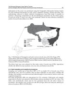
, see Figure 1.
Fig. 1. Geometry of scattering by an atmospheric volume element. The volume element is
located in the origin
In Figure 1 the local zenith and the incident and scattered light rays define three points on
the unit circle. Applying the sine rule to this spherical triangle (thicker curves in the figure)
yields.
sin sin( )
cos
sin
i i
x
sin( )
sin( )
2
sin sin
i
i
x
(6)
Therefore polarization angle
x
, i.e., the angle between the polarization plane and the local
meridian plane, is given by
Remotesensingofaerosolovervegetation
coverbasedonpixellevelmulti-wavelengthpolarizedmeasurements 317
reflectance acquired over various vegetative cover. We found that the polarization
characteristics of the surface concerned with the physical and chemical properties,
wavelength and the geometric structure factors. Moreover, we also found that under the
same observation geometric conditions, the Change of polarization characteristics caused by
the surface geometric structure could be effectively removed by computing the ratio
between the short wave infrared bands (SWIR) polarized reflectance with those in the
visible channels, especially over crop canopies surface. For this crop canopies studied, our
results suggest that using this kind of the correlation between the SWIR polarized
reflectance with those in the visible can precisely eliminate the effect of surface polarized
characteristic which caused by the vegetative surface geometric structure. The algorithm of
computing the ratio of polarization bands have been applied to satellite polarization
datasets to solve the inverse problem of separating the surface and atmospheric scattering
contributions over land surface covered vegetation. The results suggest that compared to
using a typically based on theoretical modeling to represent complex ground surface, the
method does not require the ground polarized reflectance and minimizes the effect of land
surface. This makes it possible to accurately discriminating the aerosol contribution from the
ground surface in the retrieval procedure.
2. Theory and backgrand
Polarization (Brit. polarisation) is a property of waves that describes the orientation of their
oscillations. The polarization is described by specifying the direction of the wave's electric
field. According to the Maxwell equations, the direction of the magnetic field is uniquely
determined for a specific electric field distribution and polarization. The simplest
manifestation of polarization to visualize is that of a plane wave, which is a good
approximation of most light waves. For plane waves the transverse condition requires that
the electric and magnetic field be perpendicular to the direction of propagation and to each
other. Conventionally, when considering polarization, the electric field vector is described
and the magnetic field is ignored since it is perpendicular to the electric field and
proportional to it. The electric field vector of a plane wave may be arbitrarily divided into
two perpendicular components labeled x (0
0
) and y (90
0
) (with z indicating the direction of
travel). The two components have exactly the same frequency. However, these components
have two other defining characteristics that can differ. First, the two components may not
have the same amplitude. Second, the two components may not have the same phase. That
is they may not reach their maxima and minima at the same time.
Although direct, unscattered sunlight is unpolarized, sunlight reflected by the Earth’s
atmosphere is generally polarized because of scattering by atmospheric gaseous molecules
and aerosol particles. Linearly polarized light can be described by the Stokes parameters
(The Stokes parameters are a set of values that describe the polarization state of
electromagnetic radiation (including visible light). They were defined by George Gabriel
Stokes in 1852) I, Q, and U, which are defined, relative to any reference plane, as follows:
I=I0°+ I90° (1)
Q=I0°-I90°
(2)
U=I45°-135° (3)
where I is the total intensity and Q and U fully represent the linear polarization. In Eqs.(1)–
(3) the angles denote the direction of the transmission axis of a linear polarizer relative to the
reference plane. The degree of linear polarization P is given by
2 2
Q U
P
I
(4)
and the direction of polarization
x
relative to the reference plane is given by
ta n 2
U
x
Q
(5)
For the unique definition of
x
, see Figure 1.
Fig. 1. Geometry of scattering by an atmospheric volume element. The volume element is
located in the origin
In Figure 1 the local zenith and the incident and scattered light rays define three points on
the unit circle. Applying the sine rule to this spherical triangle (thicker curves in the figure)
yields.
sin sin( )
cos
sin
i i
x
sin( )
sin( )
2
sin sin
i
i
x
(6)
Therefore polarization angle
x
, i.e., the angle between the polarization plane and the local
meridian plane, is given by
GeoscienceandRemoteSensing,NewAchievements318
sin sin( )
cos
sin
i i
x
(7)
The zenith and azimuth angles of the incident sunlight are
( , )
i i
, and the zenith and
azimuth angles of the scattered light ray (the observer) are
( , )
. The solar zenith angle
is
0 i
. With these definitions, scattering angle
is given by
cos cos cos sin sin cos( )
i i i
,
0
(8)
3. Aerosol Polarization
From Mie calculation of the light scattered by spherical particles with dimensions
representative of terrestrial aerosols, one can guess that polarization should be very
informative about the particle size distribution and refractive index. Inversely, because
polarization is very sensitive to the particle properties, this information is nearly untractable
without a priori knowledge of the particle shape (Mishchenko and Travis, 1994). Over the
past decades, considerable effort has been devoted to the study of aerosol polarization
properties. One uses appropriate radiative transfer calculations to evaluate the contribution
of aerosol polarization scattering. The aerosol’s size distribution and refractive index are
derived simultaneously from their scattering properties.
The simulations are performed by a successive order of scattering (SOS) code. We assume a
plane-parallel atmosphere on top of a Lambertian ground surface with uniform
reflectance
0.3
and a bi-direction reflectance with BPDF model, a typical and bi-direction
reflectance value of ground reflectance at the near-infrared wavelength considered. The
aerosols are mixed uniformly with the molecules. The code accounts for multiple scattering
by molecules and aerosols and reflection on the surface. Polarization ellipticity is neglected.
The results are expressed in terms of polarized radiance Lp, defined by
2 2
L
p Q U
(9)
3.1 Relationship between aerosol polarization phase function
and particle physical properties
Aerosol polarization phase function is known to be highly sensitive to aerosol optical
properties, especially aerosol absorption properties, as was shown by Vermeulen et al [6]
and Li et al [7]. Polarization phase function provided important information for aerosol
scattering properties. Figure 2(a) [Li et al]shows the calculated polarization phase function
in the principal plane as a function of the scattering angle. The calculations correspond to
those for aerosol with four types of refractive index and the size distribution given by the
bimodal log-normal model for sensitivity of polarization phase function to the aerosol real
(scattering ) and imaginary (absorption) part of refractive index. It can be seen from
Figure 2(a) that the aerosol refractive index (including real and imaginary part) is highly
sensitive to polarized phase function. Typically, we consider that the difference among
polarized phase function curves of various aerosol refractive index at the range of scattering
angle 30
0
90
0
is quite significant, showing a characteristic of the sensitivity of aerosol
polarized phase function to refractive index. Moreover, the maximum value at the scattering
angle from 30
0
to 90
0
is more accessible in the principal-plane geometry.
For the size distribution model of aerosol particle, Figure 2(b) is the curve of polarized phase
function of three size distribution models with the same index of refractive. It can be seen
from Figure 2(b) that the aerosol size distribution models is also highly sensitive to
polarized phase function[7]. The aerosol size distribution models can significantly affect the
polarization function. That is to say, the polarization phase function of aerosol can be used
to be important information to retrieve the size distribution model of aerosol.
Fig. 2(a) Fig. 2(b)
3.2 Polarization radiance response to aerosol optical thickness and wave lengths
Aerosol polarization radiance is sensitive to aerosol optical thickness. For remote sensing of
aerosol, polarization radiance is nearly additive with respect to the contributions of
molecules, aerosols. Figure 2(c) shows the calculated aerosol polarization radiance in the
principal plane as a function of the observation zenith angle. The curves of the aerosol
polarized radiance are calculated at 865nm, for different aerosol optical thickness with the
size distribution given by the bimodal log-normal model for the sensitivity of aerosol
polarization radiance to the aerosol optical thickness. It can be seen from Figure 2(c) that the
aerosol polarization radiance is highly sensitive to aerosol optical thickness. Aerosol optical
thickness can be derived from aerosol polarization radiance measurements. Aerosol
polarization measurements can be used to retrieve the aerosol optical properties.
For the spectral wavelength, Figure 2(d) shows typical results for the sensitivity of aerosol
polarized radiance to the spectral wavelength. The different curves correspond to different
aerosol polarized radiance at 865nm, 670nm and 1640nm. It can be seen from Figure 2(d)
and 3(d) that polarization will allow to retrieve aerosol key parameters concerning spectral
wavelength.
Remotesensingofaerosolovervegetation
coverbasedonpixellevelmulti-wavelengthpolarizedmeasurements 319
sin sin( )
cos
sin
i i
x
(7)
The zenith and azimuth angles of the incident sunlight are
( , )
i i
, and the zenith and
azimuth angles of the scattered light ray (the observer) are
( , )
. The solar zenith angle
is
0 i
. With these definitions, scattering angle
is given by
cos cos cos sin sin cos( )
i i i
,
0
(8)
3. Aerosol Polarization
From Mie calculation of the light scattered by spherical particles with dimensions
representative of terrestrial aerosols, one can guess that polarization should be very
informative about the particle size distribution and refractive index. Inversely, because
polarization is very sensitive to the particle properties, this information is nearly untractable
without a priori knowledge of the particle shape (Mishchenko and Travis, 1994). Over the
past decades, considerable effort has been devoted to the study of aerosol polarization
properties. One uses appropriate radiative transfer calculations to evaluate the contribution
of aerosol polarization scattering. The aerosol’s size distribution and refractive index are
derived simultaneously from their scattering properties.
The simulations are performed by a successive order of scattering (SOS) code. We assume a
plane-parallel atmosphere on top of a Lambertian ground surface with uniform
reflectance
0.3
and a bi-direction reflectance with BPDF model, a typical and bi-direction
reflectance value of ground reflectance at the near-infrared wavelength considered. The
aerosols are mixed uniformly with the molecules. The code accounts for multiple scattering
by molecules and aerosols and reflection on the surface. Polarization ellipticity is neglected.
The results are expressed in terms of polarized radiance Lp, defined by
2 2
L
p Q U
(9)
3.1 Relationship between aerosol polarization phase function
and particle physical properties
Aerosol polarization phase function is known to be highly sensitive to aerosol optical
properties, especially aerosol absorption properties, as was shown by Vermeulen et al [6]
and Li et al [7]. Polarization phase function provided important information for aerosol
scattering properties. Figure 2(a) [Li et al]shows the calculated polarization phase function
in the principal plane as a function of the scattering angle. The calculations correspond to
those for aerosol with four types of refractive index and the size distribution given by the
bimodal log-normal model for sensitivity of polarization phase function to the aerosol real
(scattering ) and imaginary (absorption) part of refractive index. It can be seen from
Figure 2(a) that the aerosol refractive index (including real and imaginary part) is highly
sensitive to polarized phase function. Typically, we consider that the difference among
polarized phase function curves of various aerosol refractive index at the range of scattering
angle 30
0
90
0
is quite significant, showing a characteristic of the sensitivity of aerosol
polarized phase function to refractive index. Moreover, the maximum value at the scattering
angle from 30
0
to 90
0
is more accessible in the principal-plane geometry.
For the size distribution model of aerosol particle, Figure 2(b) is the curve of polarized phase
function of three size distribution models with the same index of refractive. It can be seen
from Figure 2(b) that the aerosol size distribution models is also highly sensitive to
polarized phase function[7]. The aerosol size distribution models can significantly affect the
polarization function. That is to say, the polarization phase function of aerosol can be used
to be important information to retrieve the size distribution model of aerosol.
Fig. 2(a) Fig. 2(b)
3.2 Polarization radiance response to aerosol optical thickness and wave lengths
Aerosol polarization radiance is sensitive to aerosol optical thickness. For remote sensing of
aerosol, polarization radiance is nearly additive with respect to the contributions of
molecules, aerosols. Figure 2(c) shows the calculated aerosol polarization radiance in the
principal plane as a function of the observation zenith angle. The curves of the aerosol
polarized radiance are calculated at 865nm, for different aerosol optical thickness with the
size distribution given by the bimodal log-normal model for the sensitivity of aerosol
polarization radiance to the aerosol optical thickness. It can be seen from Figure 2(c) that the
aerosol polarization radiance is highly sensitive to aerosol optical thickness. Aerosol optical
thickness can be derived from aerosol polarization radiance measurements. Aerosol
polarization measurements can be used to retrieve the aerosol optical properties.
For the spectral wavelength, Figure 2(d) shows typical results for the sensitivity of aerosol
polarized radiance to the spectral wavelength. The different curves correspond to different
aerosol polarized radiance at 865nm, 670nm and 1640nm. It can be seen from Figure 2(d)
and 3(d) that polarization will allow to retrieve aerosol key parameters concerning spectral
wavelength.
GeoscienceandRemoteSensing,NewAchievements320
Fig. 2(c) Fig. 2(d)
4. Vegetation Polarization model
In the remote sensing of aerosol over land surface, a parameterization of the surface
polarized reflectance is needed for the characterization of atmospheric aerosol over land
surface. Because the aerosols properties are efficient at polarizing scattered light. Whereas
the surface reflectance is little polarized, that is the reason why the polarization
measurements can be used to estimate the atmospheric aerosol properties over land surface
[2]. Although small, the surface contribution to the top of the atmosphere (TOA) polarized
reflectance cannot be neglected and some parameterization is required. In addition, the
parameter of the surface is used as a boundary condition for solving vector radiative
transfer (VRT) in both direct and inverse problems. In general, the bidirectional polarization
distribution functions (BPDF) is used to estimate the atmospheric contribution to the TOA
signal. The function will be used as a boundary condition for the estimate of atmospheric
aerosol from polarization remote sensing measurements over land surface.
In most cases, measurements of linear polarization of solar radiation reflected by a plant
canopy just provide a simple and relatively cheap way to obtain the characterization of a
plant canopy polarized reflectance. Although it demonstrates the relationships between
polarized light scattering properties and plant canopies properties, more research is needed
if the complexity and diversity inherent in plant canopies is to be modeled, especially more
practical BPDF model as a boundary condition for the estimate of atmospheric aerosol.
For remote sensing of aerosol over land surface including polarization information, the
vector radiative transfer equation accounting for radiation polarization provides the power
simulation of a satellite signal in the solar spectrum in a mixed molecular-aerosol
atmosphere and surface polarized reflectance. In order to present the characterization of the
TOA polarized reflectance of vegetated surface, some simulation accounting for radiation
polarization in atmosphere and surface were made. In what follows, we used the method of
successive orders of scattering (SOS) approximations to compute photons scattered one,
two, three times, and etc. Rondeaux’s , Breon’s and Nadal’s BPDF models were used to
calculate the contribution of the land surface covered plant canopies polarized reflectance as
a boundary condition to solve vector radiative transfer equation. It is noticed that:
4.1 The TOA polarized reflectance of vegetation cover depends
on zenith angle of sunlight.
Upward polarization radiation at the top of the atmosphere was computed by the successive
orders of scattering (SOS) approximations method for wavelengths (
) of 443 m
.
Polarization radiation at the TOA varies according to the angle of incidence. As shows in
Figure 3(a) and (b).
Fig. 3(a) Fig. 3(b)
4.2 Surface BPDF with different land cover types or model
Characterization of the polarizing properties of land surfaces raises probably a more
complicated problem than for the atmosphere, on account of the large diversity of ground
targets. Concerning the underlying polarizing mechanism, it is usually admitted that land
surfaces are partly composed of elementary specular reflectors (water facets, leaves, small
mineral surfaces) which, according to Fresnel’s law, reflect partially polarized light when
illuminated by the direct sunbeam. There is convincing evidence that it is correct in the
important case of vegetation cover [Vanderbilt and Grant, 1985; Vanderbilt et al., 1985;
Rondeaux and herman, 1991]. By assuming this hypothesis and restricting to singly reflected
light, we can anticipate that the main parameters governing the land surface bidirectional
polarization distribution function (BPDF), apart from the Fresnel coefficients for reflection,
should be the relative surface occupied by specular reflectors, the distribution function of
the orientation of these reflectors, and the shadowing effects resulting from the medium
structure [7]. Plant canopies structure is difficult to model with single BPDF.
As example of land surface canopy BPDF predicted within this context, we consider the
TOA polarized radiance contribution of the model for vegetative cover depends on canopy
structure, cellular pigments and refractive indices of vegetation, as the Figure 3(c) and (d)
shown. It can be seen in Figure 3(c) that the polarized radiance distribution in 2
space is
controlled by directions of both incidence and reflection, and by the main parameters
governing the vegetative structures. Comparison of Figure 3(c) and Figure 3(d) shows that
according to difference of the refractive indices, the reflective distribution of the polarized
radiance varies correspondingly.
Remotesensingofaerosolovervegetation
coverbasedonpixellevelmulti-wavelengthpolarizedmeasurements 321
Fig. 2(c) Fig. 2(d)
4. Vegetation Polarization model
In the remote sensing of aerosol over land surface, a parameterization of the surface
polarized reflectance is needed for the characterization of atmospheric aerosol over land
surface. Because the aerosols properties are efficient at polarizing scattered light. Whereas
the surface reflectance is little polarized, that is the reason why the polarization
measurements can be used to estimate the atmospheric aerosol properties over land surface
[2]. Although small, the surface contribution to the top of the atmosphere (TOA) polarized
reflectance cannot be neglected and some parameterization is required. In addition, the
parameter of the surface is used as a boundary condition for solving vector radiative
transfer (VRT) in both direct and inverse problems. In general, the bidirectional polarization
distribution functions (BPDF) is used to estimate the atmospheric contribution to the TOA
signal. The function will be used as a boundary condition for the estimate of atmospheric
aerosol from polarization remote sensing measurements over land surface.
In most cases, measurements of linear polarization of solar radiation reflected by a plant
canopy just provide a simple and relatively cheap way to obtain the characterization of a
plant canopy polarized reflectance. Although it demonstrates the relationships between
polarized light scattering properties and plant canopies properties, more research is needed
if the complexity and diversity inherent in plant canopies is to be modeled, especially more
practical BPDF model as a boundary condition for the estimate of atmospheric aerosol.
For remote sensing of aerosol over land surface including polarization information, the
vector radiative transfer equation accounting for radiation polarization provides the power
simulation of a satellite signal in the solar spectrum in a mixed molecular-aerosol
atmosphere and surface polarized reflectance. In order to present the characterization of the
TOA polarized reflectance of vegetated surface, some simulation accounting for radiation
polarization in atmosphere and surface were made. In what follows, we used the method of
successive orders of scattering (SOS) approximations to compute photons scattered one,
two, three times, and etc. Rondeaux’s , Breon’s and Nadal’s BPDF models were used to
calculate the contribution of the land surface covered plant canopies polarized reflectance as
a boundary condition to solve vector radiative transfer equation. It is noticed that:
4.1 The TOA polarized reflectance of vegetation cover depends
on zenith angle of sunlight.
Upward polarization radiation at the top of the atmosphere was computed by the successive
orders of scattering (SOS) approximations method for wavelengths (
) of 443 m
.
Polarization radiation at the TOA varies according to the angle of incidence. As shows in
Figure 3(a) and (b).
Fig. 3(a) Fig. 3(b)
4.2 Surface BPDF with different land cover types or model
Characterization of the polarizing properties of land surfaces raises probably a more
complicated problem than for the atmosphere, on account of the large diversity of ground
targets. Concerning the underlying polarizing mechanism, it is usually admitted that land
surfaces are partly composed of elementary specular reflectors (water facets, leaves, small
mineral surfaces) which, according to Fresnel’s law, reflect partially polarized light when
illuminated by the direct sunbeam. There is convincing evidence that it is correct in the
important case of vegetation cover [Vanderbilt and Grant, 1985; Vanderbilt et al., 1985;
Rondeaux and herman, 1991]. By assuming this hypothesis and restricting to singly reflected
light, we can anticipate that the main parameters governing the land surface bidirectional
polarization distribution function (BPDF), apart from the Fresnel coefficients for reflection,
should be the relative surface occupied by specular reflectors, the distribution function of
the orientation of these reflectors, and the shadowing effects resulting from the medium
structure [7]. Plant canopies structure is difficult to model with single BPDF.
As example of land surface canopy BPDF predicted within this context, we consider the
TOA polarized radiance contribution of the model for vegetative cover depends on canopy
structure, cellular pigments and refractive indices of vegetation, as the Figure 3(c) and (d)
shown. It can be seen in Figure 3(c) that the polarized radiance distribution in 2
space is
controlled by directions of both incidence and reflection, and by the main parameters
governing the vegetative structures. Comparison of Figure 3(c) and Figure 3(d) shows that
according to difference of the refractive indices, the reflective distribution of the polarized
radiance varies correspondingly.
GeoscienceandRemoteSensing,NewAchievements322
Fig. 3(c) Fig. 3(d)
4.3 Retrieval of TOA contribution of aerosol and land surface polarization
The TOA measured polarized radiance is the sum of 3 contributions: aerosol scattering,
Rayleigh scattering, and the reflection of sun light by the land surface, attenuated by the
atmospheric transmission on the down-welling and upwelling paths. In order to find out the
influence of aerosol and land surface polarization on the TOA polarized contribution, we
choose different aerosol model and aerosol optical thickness at a certain land surface BPDF
model condition as study parameters.
In this study, the contribution of land surface was calculated by BPDF derived from ground-
based measurements for vegetative cover [Rondeaux and herman, 1991], for the
atmospheric aerosol, an externally mixed model of these aerosol components is assumed
[15]. The size distribution for each aerosol model is expressed by the log-normal function,
2
2
(ln ln )
( ) 1
exp( )
ln 2 ln
2 ln
m
r r
dn r
d r
(10)
Where rm is the median radius and ln r is the standard deviation. The rm and r values are
0.3
m
and 2.51
m
for the OC model [5], the refractive indices at 443 m
is 1.38±i8.01 for
the OC model, and 1.53±i0.005 and 1.52±i0.012 for the WS model. The scattering matrices are
computed by the Mie scattering theory for radii ranging from 0.001 to 10.0
m
assuming the
shape of aerosol particles to be spherical. We can see from the experiment result that the
TOA polarized radiance in 2
space is obvious difference, varying according to the aerosol
optical thickness Figure 3(e) and 3(f). Comparison of Figure 3(g) and 3(h) also shows that
this difference in aerosol model implies influence on polarized radiance distribution in
2
space. Clearly, different assumptions about the aerosol model have large difference in
the TOA polarized radiance.
Fig. 3(e) aerosol optical depth is 0.2 Fig. 3(f) aerosol optical depth is 0.5
Fig. 3(g) Aerosol model is Jung model Fig. 3(h) aerosol model is WMO
4. Based on short-wave infrared band polarized model
Solar light reflected by natural surfaces is partly polarized. The degree of polarization, and
the polarization direction, may yield some information about the surface such as its
roughness, its water content, or the leaf inclination distribution. It is believed that polarized
light is generated at the surface by specular reflection on the leaf surfaces. This hypothesis
has been used to elaborate analytical models for the polarized reflectance of vegetation.
Because of this fact and because the refractive index of natural targets (e.g. leaf of
vegetation) varies little within the spectral domain of interest (visible and near IR), the
surface polarized reflectance is spectrally neutral, in contrast with the total reflectance.
Based on this polarization information and the requirement of the surface polarized
reflectance, we can choose to study space-borne polarized reflectance with multi-
wavelengths and multi-direction measurements.
The observations of the earth from space that have included polarization measurements are
those in an exploratory project aboard the space Shuttle (Coulson et at. ,1986). By the nature
Remotesensingofaerosolovervegetation
coverbasedonpixellevelmulti-wavelengthpolarizedmeasurements 323
Fig. 3(c) Fig. 3(d)
4.3 Retrieval of TOA contribution of aerosol and land surface polarization
The TOA measured polarized radiance is the sum of 3 contributions: aerosol scattering,
Rayleigh scattering, and the reflection of sun light by the land surface, attenuated by the
atmospheric transmission on the down-welling and upwelling paths. In order to find out the
influence of aerosol and land surface polarization on the TOA polarized contribution, we
choose different aerosol model and aerosol optical thickness at a certain land surface BPDF
model condition as study parameters.
In this study, the contribution of land surface was calculated by BPDF derived from ground-
based measurements for vegetative cover [Rondeaux and herman, 1991], for the
atmospheric aerosol, an externally mixed model of these aerosol components is assumed
[15]. The size distribution for each aerosol model is expressed by the log-normal function,
2
2
(ln ln )
( ) 1
exp( )
ln 2 ln
2 ln
m
r r
dn r
d r
(10)
Where rm is the median radius and ln r is the standard deviation. The rm and r values are
0.3
m
and 2.51
m
for the OC model [5], the refractive indices at 443 m
is 1.38±i8.01 for
the OC model, and 1.53±i0.005 and 1.52±i0.012 for the WS model. The scattering matrices are
computed by the Mie scattering theory for radii ranging from 0.001 to 10.0
m
assuming the
shape of aerosol particles to be spherical. We can see from the experiment result that the
TOA polarized radiance in 2
space is obvious difference, varying according to the aerosol
optical thickness Figure 3(e) and 3(f). Comparison of Figure 3(g) and 3(h) also shows that
this difference in aerosol model implies influence on polarized radiance distribution in
2
space. Clearly, different assumptions about the aerosol model have large difference in
the TOA polarized radiance.
Fig. 3(e) aerosol optical depth is 0.2 Fig. 3(f) aerosol optical depth is 0.5
Fig. 3(g) Aerosol model is Jung model Fig. 3(h) aerosol model is WMO
4. Based on short-wave infrared band polarized model
Solar light reflected by natural surfaces is partly polarized. The degree of polarization, and
the polarization direction, may yield some information about the surface such as its
roughness, its water content, or the leaf inclination distribution. It is believed that polarized
light is generated at the surface by specular reflection on the leaf surfaces. This hypothesis
has been used to elaborate analytical models for the polarized reflectance of vegetation.
Because of this fact and because the refractive index of natural targets (e.g. leaf of
vegetation) varies little within the spectral domain of interest (visible and near IR), the
surface polarized reflectance is spectrally neutral, in contrast with the total reflectance.
Based on this polarization information and the requirement of the surface polarized
reflectance, we can choose to study space-borne polarized reflectance with multi-
wavelengths and multi-direction measurements.
The observations of the earth from space that have included polarization measurements are
those in an exploratory project aboard the space Shuttle (Coulson et at. ,1986). By the nature
GeoscienceandRemoteSensing,NewAchievements324
of the problem, however, solar radiation directed to space at the level of the Shuttle and
other spacecraft contains a significant component due to scattering by the atmosphere,
meanwhile that due to surface reflection. For atmospheric characterization and
discrimination, however, such surface reflection contamination of the radiation field should
be minimized or corrected for by use of radiative transfer models applicable to the
conditions of observation. For maximum information content, of course, both intensity and
state of polarization of the scattering by the atmosphere should be included.
Light would consist of components
E
and
E
, normal and parallel, respectively, to the
principal plane. Fresnel’s laws of reflection give the reflected electric intensity components.
sin( )
sin( )
E E
(11)
( )
( )
tg
E
E
tg
(12)
Thus from the definition of the Fresnel degree of polarization, we have
2 2
2 2
2 2
2 2
2 2
2 2
2 2
2 2
sin ( ) ( )
sin ( ) ( )
sin ( ) ( )
sin ( ) ( )
tg
E E
E E
tg
P
tg
E E
E E
tg
(13)
Since Fresnel’s laws of refraction, in which case Eq. (11) and Eq. (12) reduces to
2 2
2 2
s i n c o s
s i n c o s
E N
E
N
(14)
2 2 2
2 2 2
c o s s in
c o s s in
E
N N
E
N N
(15)
Obviously, for unpolarized light
2
E
=
2
E
, for convenience, we summarize the relations
Eq.(13) and Eq. (14) as follows:
2
2 2
2
2 2 2
2 2 2 2
2 2
2 2
sin sin
2 cos 1 sin
2 sin sin
sin sin
sin sin
cos sin
tg N
N N
P
N
N tg
N N
(16)
Here N is the index of refraction of the medium, and
is the angle of incidence or
reflection. The index of refraction
N is related to the wavelength.
This shows that the degree of polarization is related to the wavelength and the angle of
incidence or reflection Figure 4(a). Furthermore, under the same observation geometric
conditions, this important relationship also shows that the degree of polarization of the
SWIR (short wave infrared band) is related to that of the visible rang Figure 4(b).
Fig. 4(a) Fig. 4(b)
Figure 4(a) shows the relationship between degree of polarization and wavelengths and the
angle of incidence or reflection and (b) between degree of polarization at long wavelengths
1640nm and that at short wavelengths
In Figure 4(b), we found that the SWIR is similar to the visible channels by polarized. That
is, the polarized reflectance in SWIR could be used similarly to quantify that in the visible
wavelength. This fact would find important applications in solving the inverse problem of
separating the surface and atmospheric scattering contributions.
With these and atmospheric conditions, we find, after some algebraic manipulation that
( ) /
( ) /
1 2
( ) /
( , ) * ( , )
( , ) * ( , )
*
s sw ir s
s vi s
u
p swir p swir
sw ir
u
vi p vi p vi
s
u
R e R
L
L R e R
e
(17)
Where
( , )
P
R
is given by
2 2
2 2 2 2 2
2 2 2 2 2
1
( , )
2
sin cos cos sin
sin cos cos sin
P
R
N N N
N N N
(18)
Where
s
wir
L
and
vi
L
are the polarized reflected radiance at long wavelengths and that at short
wavelengths, respectively,
is the scattering angle, and
is atmospheric optical thickness.
The principle of the algorithm can be seen in Eq. (17). The relationship of the degree of
polarization between two wavelengths (the visible rang and short wave infrared band) from
Remotesensingofaerosolovervegetation
coverbasedonpixellevelmulti-wavelengthpolarizedmeasurements 325
of the problem, however, solar radiation directed to space at the level of the Shuttle and
other spacecraft contains a significant component due to scattering by the atmosphere,
meanwhile that due to surface reflection. For atmospheric characterization and
discrimination, however, such surface reflection contamination of the radiation field should
be minimized or corrected for by use of radiative transfer models applicable to the
conditions of observation. For maximum information content, of course, both intensity and
state of polarization of the scattering by the atmosphere should be included.
Light would consist of components
E
and
E
, normal and parallel, respectively, to the
principal plane. Fresnel’s laws of reflection give the reflected electric intensity components.
sin( )
sin( )
E E
(11)
( )
( )
tg
E
E
tg
(12)
Thus from the definition of the Fresnel degree of polarization, we have
2 2
2 2
2 2
2 2
2 2
2 2
2 2
2 2
sin ( ) ( )
sin ( ) ( )
sin ( ) ( )
sin ( ) ( )
tg
E E
E E
tg
P
tg
E E
E E
tg
(13)
Since Fresnel’s laws of refraction, in which case Eq. (11) and Eq. (12) reduces to
2 2
2 2
s i n c o s
s i n c o s
E N
E
N
(14)
2 2 2
2 2 2
c o s s in
c o s s in
E
N N
E
N N
(15)
Obviously, for unpolarized light
2
E
=
2
E
, for convenience, we summarize the relations
Eq.(13) and Eq. (14) as follows:
2
2 2
2
2 2 2
2 2 2 2
2 2
2 2
sin sin
2 cos 1 sin
2 sin sin
sin sin
sin sin
cos sin
tg N
N N
P
N
N tg
N N
(16)
Here N is the index of refraction of the medium, and
is the angle of incidence or
reflection. The index of refraction
N is related to the wavelength.
This shows that the degree of polarization is related to the wavelength and the angle of
incidence or reflection Figure 4(a). Furthermore, under the same observation geometric
conditions, this important relationship also shows that the degree of polarization of the
SWIR (short wave infrared band) is related to that of the visible rang Figure 4(b).
Fig. 4(a) Fig. 4(b)
Figure 4(a) shows the relationship between degree of polarization and wavelengths and the
angle of incidence or reflection and (b) between degree of polarization at long wavelengths
1640nm and that at short wavelengths
In Figure 4(b), we found that the SWIR is similar to the visible channels by polarized. That
is, the polarized reflectance in SWIR could be used similarly to quantify that in the visible
wavelength. This fact would find important applications in solving the inverse problem of
separating the surface and atmospheric scattering contributions.
With these and atmospheric conditions, we find, after some algebraic manipulation that
( ) /
( ) /
1 2
( ) /
( , ) * ( , )
( , ) * ( , )
*
s sw ir s
s vi s
u
p swir p swir
sw ir
u
vi p vi p vi
s
u
R e R
L
L R e R
e
(17)
Where
( , )
P
R
is given by
2 2
2 2 2 2 2
2 2 2 2 2
1
( , )
2
sin cos cos sin
sin cos cos sin
P
R
N N N
N N N
(18)
Where
s
wir
L
and
vi
L
are the polarized reflected radiance at long wavelengths and that at short
wavelengths, respectively,
is the scattering angle, and
is atmospheric optical thickness.
The principle of the algorithm can be seen in Eq. (17). The relationship of the degree of
polarization between two wavelengths (the visible rang and short wave infrared band) from
GeoscienceandRemoteSensing,NewAchievements326
the radiative transfer calculation is shown as a function of the aerosol optical thickness at the
visible rang and the short wave infrared band.
5. Based on pixel-level multi-angle remote sensing of aerosol
The first space-based polarization measurements were undertaken by ADEOS/POLDER.
The POLDER has supplied the observed data not only in the multi-wavelength bands but
also at the multi-viewing angles. These directional measurements include significant
information of atmospheric aerosols. This work is a feasibility study of multi-directional
data for the retrieval of aerosols characteristics. The basic algorithm for aerosol retrieval is
based on light scattering simulations of polarization field, where the heterogeneous aerosol
model according to Maxwell-Garnett mixing rule is considered. It is shown that polarization
data observed at multi-angles is a powerful tool to retrieve aerosol characteristics.
The information provided polarization space-borne sensor permit the development of a new
approach to retrieving the aerosol loading at a global scale. The main contribution to the
TOA polarized radiance at short wavelengths is due to the aerosols and molecules of the
atmosphere, while the contribution of the surface is generally smaller than that of the
aerosols. The contribution of atmospheric molecules, although significant at short
wavelengths, is nearly invariant and can be easily modeled. That of the surface is more
variable but the Eq. (17) and Eq. (18) show that it can be modeled with the polarized
reflectance in SWIR, since the contribution of atmospheric aerosol at long wavelengths is
generally small and always possible to be negligible. The contribution of the surface at long
wavelengths could be used similarly to quantify that at short wavelength. Thus, the aerosol
contribution to the polarized radiance can in principle be extracted from the measurement
with computing the ratio between the SWIR ground polarized reflectance and those in the
visible channels.
The measured polarized radiance
p
ol
L
is modeled as
p
ol aer mol surf
L L L L
(19)
that is, the sum of 3 contributions :
aer
L
, generated by aerosol single scattering,
mol
L
, by
Rayleigh scattering, and
s
urf
L
, due to the reflection of sun light by the surface, attenuated by
the atmospheric transmission on the down-welling and upwelling paths. These terms are
expressed as:
( )
( , , , ) ( , , )
4 cos
a s
aer s v a
v
E
L
Q n
(20)
( )
( , , , ) ( , )
4 cos
m s
mol s v m
v
E
L Q
(21)
1 1
( , , , ) cos ( , ) * exp( ( )( ))
cos cos
s
surf s v s p m
v s
E
L R
(22)
Where
( )
a
and
( )
m
are the optical thickness of the aerosols and of the molecules,
respectively.
s
E
is the TOA solar irradiance.
( , )
m
Q
and
( , , )
a
Q n
are pre-calculated
functions, which depend on the geometric angles
s
,
v
,
only through the scattering
angle
. By performing some algebraic manipulation from Eq. (17)-(22), it is seen that the
contribution of the surface at short wavelengths could be quantified with that at long
wavelengths.
Inversions were performed with this important relationship. The TOA Polarized reflectance
measurements were screened for cloud contamination and corrected for gas absorption.
Based on lookup tables composed of optical contributions from mono-modal lognormal
aerosol size distributions with fixed standard deviations, but with several values of the
modal radius and refractive index, we made use of one week of space-borne POLDER
acquisition on from November 7 to 12 , 2007 Beijing China, (latitude 39
0
58’37’’, longitude
116
0
22’51’’). The retrieval method described above for AOD from POLDER yields the AOD
composite images of Figure 5a.
In order to analyze the accuracy of aerosol inversion, we interpolated the AERONET AOD
corresponding to time of the satellite overpass. We used the data provided by Beijing
AERONET stations to analyze the accuracy of aerosol inversion from POLDER. Figure 5b
shows the results. The validation shown in Figure 5b compares the AOD at 865nm derived
from POLDER and AERONET instruments. As the result shows (Figure 5b), the retrieval
method for the AOD from POLDER yields a nearly closer values compared with that from
AERONET.
6. Summary
In this paper, the accuracy of AOD retrieved from the POLDER multi-wavelengths-based
inversion scheme for the sample studied over Beijing remain relatively closer compared to
Fig. 6a the composite images of aerosol
optical thickness
Fig. 6b compared AOD derived
from POLDER and AERONET
Remotesensingofaerosolovervegetation
coverbasedonpixellevelmulti-wavelengthpolarizedmeasurements 327
the radiative transfer calculation is shown as a function of the aerosol optical thickness at the
visible rang and the short wave infrared band.
5. Based on pixel-level multi-angle remote sensing of aerosol
The first space-based polarization measurements were undertaken by ADEOS/POLDER.
The POLDER has supplied the observed data not only in the multi-wavelength bands but
also at the multi-viewing angles. These directional measurements include significant
information of atmospheric aerosols. This work is a feasibility study of multi-directional
data for the retrieval of aerosols characteristics. The basic algorithm for aerosol retrieval is
based on light scattering simulations of polarization field, where the heterogeneous aerosol
model according to Maxwell-Garnett mixing rule is considered. It is shown that polarization
data observed at multi-angles is a powerful tool to retrieve aerosol characteristics.
The information provided polarization space-borne sensor permit the development of a new
approach to retrieving the aerosol loading at a global scale. The main contribution to the
TOA polarized radiance at short wavelengths is due to the aerosols and molecules of the
atmosphere, while the contribution of the surface is generally smaller than that of the
aerosols. The contribution of atmospheric molecules, although significant at short
wavelengths, is nearly invariant and can be easily modeled. That of the surface is more
variable but the Eq. (17) and Eq. (18) show that it can be modeled with the polarized
reflectance in SWIR, since the contribution of atmospheric aerosol at long wavelengths is
generally small and always possible to be negligible. The contribution of the surface at long
wavelengths could be used similarly to quantify that at short wavelength. Thus, the aerosol
contribution to the polarized radiance can in principle be extracted from the measurement
with computing the ratio between the SWIR ground polarized reflectance and those in the
visible channels.
The measured polarized radiance
p
ol
L
is modeled as
p
ol aer mol surf
L L L L
(19)
that is, the sum of 3 contributions :
aer
L
, generated by aerosol single scattering,
mol
L
, by
Rayleigh scattering, and
s
urf
L
, due to the reflection of sun light by the surface, attenuated by
the atmospheric transmission on the down-welling and upwelling paths. These terms are
expressed as:
( )
( , , , ) ( , , )
4 cos
a s
aer s v a
v
E
L
Q n
(20)
( )
( , , , ) ( , )
4 cos
m s
mol s v m
v
E
L Q
(21)
1 1
( , , , ) cos ( , ) * exp( ( )( ))
cos cos
s
surf s v s p m
v s
E
L R
(22)
Where
( )
a
and
( )
m
are the optical thickness of the aerosols and of the molecules,
respectively.
s
E
is the TOA solar irradiance.
( , )
m
Q
and
( , , )
a
Q n
are pre-calculated
functions, which depend on the geometric angles
s
,
v
,
only through the scattering
angle
. By performing some algebraic manipulation from Eq. (17)-(22), it is seen that the
contribution of the surface at short wavelengths could be quantified with that at long
wavelengths.
Inversions were performed with this important relationship. The TOA Polarized reflectance
measurements were screened for cloud contamination and corrected for gas absorption.
Based on lookup tables composed of optical contributions from mono-modal lognormal
aerosol size distributions with fixed standard deviations, but with several values of the
modal radius and refractive index, we made use of one week of space-borne POLDER
acquisition on from November 7 to 12 , 2007 Beijing China, (latitude 39
0
58’37’’, longitude
116
0
22’51’’). The retrieval method described above for AOD from POLDER yields the AOD
composite images of Figure 5a.
In order to analyze the accuracy of aerosol inversion, we interpolated the AERONET AOD
corresponding to time of the satellite overpass. We used the data provided by Beijing
AERONET stations to analyze the accuracy of aerosol inversion from POLDER. Figure 5b
shows the results. The validation shown in Figure 5b compares the AOD at 865nm derived
from POLDER and AERONET instruments. As the result shows (Figure 5b), the retrieval
method for the AOD from POLDER yields a nearly closer values compared with that from
AERONET.
6. Summary
In this paper, the accuracy of AOD retrieved from the POLDER multi-wavelengths-based
inversion scheme for the sample studied over Beijing remain relatively closer compared to
Fig. 6a the composite images of aerosol
optical thickness
Fig. 6b compared AOD derived
from POLDER and AERONET
GeoscienceandRemoteSensing,NewAchievements328
ground-based sun-photometer measurements. The comparisons between the AERONET
AOD and the POLDER-derived AOD using the relations between the polarized reflectance
of the surface at long wavelengths and that at short wavelengths show an agreement in
most cases. The agreement is much better than when using the physical functions which
were derived for bare soils and vegetation. Some effect caused by the surface geometric
structure can precisely eliminate for dense vegetation cover or for bare soils at least.
The results suggest that the algorithm, the contribution of the surface at short wavelengths
could be quantified with that at long wavelengths in pixel level, can be used as an
alternative method in the aerosol retrieval procedure from Multi-wavelength polarization
space-borne sensors.
The POLDER results also provide convincing evidence that remote sensing of the terrestrial
aerosols over land surfaces by way of polarization measurements is feasible and possibility
for discriminating the aerosol contribution from the surface and show the potential of
measurements of polarized light scattered by aerosols to retrieve optical depth.
Acknowledgment
The paper is supported by Project supported by the Chinese Defence Advance Research
Program of Science and Technology, China (DPC, KJSX0601)
7. References
[1] A.A.Kokhanovsky, F M. Breon, A.Cacciari, et al, “Aerosol Remote Sensing over Land: A
Comparison of Satellite Retrievals using Different Algorithms and Instruments.”,
Atmospheric Research. 85, 372-394, 2007.
[2] F.Vachon, A. Royer, M. Aube, B.Toubbe, et al, “Remote Sensing of aerosols over North
American Land surfaces from POLDER and MODIS measurements”, Atmospheric
Environment Vol. 38, 3501-3515, 2004.
[3] K. Arai, Y. Iisasa, X. Liang, “Aerosol Parameter estimation with changing Observation
angle of ground based Polarization Radiometer”, Advances in Space Research. 39,
28-31, 2007.
[4] Florence Nadal and Francois-Marie Breon, “Parameterization of surface Polarized
Reflectance Derived from POLDER Space-borne measurements”, IEEE Transactions
On Geoscience and Remote Sensing. Vol. 37.NO. 3. MAY 1999.
[5] Von Hoyningen-Huene, W. Freitag, M. Burrows, J.B., et al, “Retrieval of Aerosol Optical
Thickness over Land Surface from top-of-atmosphere Radiance”, J. Geophys. Res.
108, 4260.doi:10, 1029/2001JD002018, 2003.
[6] Deuze, J.L, Breon, F.M, Devaux, C., et al, “Remote Sensing of Aerosols over Land Surface
from POLDER-ADEOS-1 Polarized Measurements”, J. Geophys. Res. 106, 4913-
4926, 2001.
[7] Li et al, “Retrieval of aerosol optical and physical properties from ground-based spectral,
multi-angular, and polarized sun-photometer measurements”, remote sensing of
environment , 101 (2006) 519-533.
Methodsandperformancesformulti-passSARInterferometry 329
Methodsandperformancesformulti-passSARInterferometry
StefanoTebaldiniandAndreaMontiGuarnieri
0
Methods and performances for
multi-pass SAR Interferometry
Stefano Tebaldini and Andrea Monti Guarnieri
Dipartimento di Elettronica e Informazione
Politecnico di Milano
Piazza Leonardo da Vinci, 32
20133 MILANO
1. Introduction
Thanks to the several space missions accomplished since ERS-1, the scientific community has
been provided with a huge amount of data suitable for interferometric processing. The in-
novation was the availability of multiple compatible images of the same areas. Such images,
achieved by looking from slightly different point of view different orbits, and/or by differ-
ent frequencies, and/or at different times, has largely extended the capabilities of InSAR with
respect to the traditional dual image case. The advantage granted by the possibility to form
multiple interferograms, instead than just one, is two folded. On the one hand, the estimation
of the parameters of interest, be them related to the DEM or the terrain deformations, is driven
by a larger data set, resulting in more accurate estimates. On the other hand, new parameters
may be added to the set of the unknowns, allowing to study complex phenomena, such as
the temporal evolution of the atmospheric and deformation fields. A major issue with multi-
image InSAR is that targets are, in general, affected by temporal and spatial decorrelation
phenomena, which hinders the exploitation of large spatial and/or temporal baselines. For
this reason, most of literature about multi-image InSAR has focused mainly on targets that stay
coherent in all the acquisitions, which has resulted in a substantial lack of a systemic approach
to deal with decorrelating targets in the field of InSAR.
The aim of this chapter is to propose a general approach to exploit all the available informa-
tion, that is the stack of interferometric SAR images, and that formally accounts for the impact
of target decorrelation. This approach is based on the optimal estimate of the data in a statis-
tical sense. The basic idea is to split the estimation process into two steps. In the first step,
a maximum likelihood (ML) estimator is used that jointly exploits all the N
× (N − 1)/2 in-
terferograms available with N acquisitions, in order to yield the best estimates of the N
− 1
phases that correspond to the optical path differences between the target and the sensors. Tar-
get decorrelation is accounted for by properly weighting each interferogram in dependence on
the target statistics. The estimated phases will be referred to as Linked Phases, to remind that
these terms are the result of the joint processing of all the N
(N − 1)/2 interferograms. Once
the first estimation step has yielded the estimates of the interferometric phases, the second
step is required to separate the contributions of the APSs and the decorrelation noise from the
parameters of interest, such as the Line of Sight Deformation Field (LDF) and the topography.
18
GeoscienceandRemoteSensing,NewAchievements330
The same two-step approach can be followed to derive the performances of the Multi-Baseline
Interferometry, in the frame of the Hybrid Cramér Rao Bound (HCRB) that we will discuss in
this same chapter.
2. A brief review of multi-image InSAR techniques
2.1 Permanent Scatterers Interferometry (PSI)
This approach, developed by Ferretti et al.(1), represents the first attempt to give a formal
framework to the problem of multi-baseline InSAR. The analysis is based on the selection of
a number of highly coherent, temporally stable, point-like targets within the imaged scene,
which may be identified by analyzing the amplitude time series extracted from the whole set
of images in correspondence with every pixel (2), (3), (4). Such targets, named Permanent
Scatterers (PS), are typically represented by man made objects, but also isolated trees or stable
rocks may serve as PSs. However, the highest density of PSs is expected to be found within
urban areas. For every selected PS the time series of the phase differences of every image
with respect to a reference one is extracted. Since the selected targets are by definition the
ones which remain coherent in all of the images, it can be assumed that no decorrelation phe-
nomena occur. Therefore, the phase difference time series may be effectively represented by
a linear model plus noise. At this point, an effective separation of the various contributions,
such as topography, displacement rate, and APSs, may be carried out by exploiting the time-
space statistical properties of each. In this sense, this approach is similar to Wiener filtering,
and could be in principle solved by such technique. However, because of the high computa-
tional burden and the non linearity due to the 2π ambiguity, Ferretti et al. proposed instead an
iterative algorithm, involving 2D frequency estimation, phase unwrapping and linear filtering
(5). The main limitation within this approach lies in the sparsity of the grid for the selected
PS. To overcome this limitation, a second step is performed, consisting in resampling the APSs
estimates on the uniform image grid, remove these terms, and look for a more dense set of PSs
basing on phase stability, rather than amplitude. This process, however, is likely to fail in ar-
eas where the initial PS selection, based on amplitude stability, does not suffice to cover the
whole imaged scene, as it may be the case of non urban areas, especially for data set suffering
from amplitude calibration problems. A first solution to this problem has been proposed by
Hooper et al. (6), who defined an iterative point selection algorithm basing directly on a phase
stability criterion. The selected point are called Persistent Scatterers. This method has been
shown to yield a more dense point grid on rock areas than the amplitude based algorithms
exploited in PSI.
2.2 Techniques based on interferogram selection
Several approaches have been presented in literature to perform SAR interferometric analysis
over scenes where the PS assumption may not be retained. A number of these works share
the idea to minimize the effect of target decorrelation by forming the interferograms from
properly selected pairs, rather than with respect to a fixed reference image, as done in PS
processing. Despite the good results achieved in the applications, however, there’s no clear
and formal assessment of the criteria which should drive the selection of the image pairs
to be used. As a result, the processing is heuristically based on the exploitation of a set of
interferograms taken with the shortest temporal and/or spatial baselines possible (7), (8), (6).
2.3 The Small Baseline Subsets (SBAS) approach
A more sophisticated approach is the one by Berardino et al., exploiting the concept of Small
Baseline Subsets (SBAS) (9), (10). This approach may be somehow considered as the comple-
ment of the PS approach. While the latter looks for targets which remain coherent throughout
the whole data set, the SBAS algorithm tries to extract information basing on every single
interferogram available. The algorithm accounts for spatial decorrelation phenomena by par-
titioning the data set into a number of subsets, each of which is constituted by images acquired
from orbits close to each other. In this way, interferograms corresponding to large baselines
are discarded. After unwrapping the phases of the interferograms within the subsets, the esti-
mation of the physical quantities of interest, such as the topographic profile and the deforma-
tion field, is carried out through singular value decomposition. The choice of this inversion
technique accounts for the rank deficiency caused by partitioning the data set into subsets,
resulting in the solution being chosen on the basis of a minimum norm criterion. Further pro-
cessing, similar to that indicated in (5), carries out the removal of the atmospheric artifacts.
2.4 Maximum Likelihood Estimation Techniques
The application of Maximum Likelihood Estimation techniques for InSAR processing has been
considered by Fornaro et al (11), De Zan (12), Rocca (13), and in two works by Tebaldini and
Monti Guarnieri (14), of which this chapter represents an extension. The rationale of ML tech-
niques, as applied to InSAR, is to exploit target statistics, represented by the ensemble of the
coherences of every available interferogram, to design a statistically optimal estimator for the
parameters of interest. An advantage granted by these techniques is that the criteria which
determine the role of each interferogram in the estimation process are directly derived from
the coherences, through a rigorous mathematical approach. Furthermore, by virtue of the
properties of the ML estimator (MLE), the estimates of the parameters of interest are asymp-
totically (we.e. large signal to noise ratio, large data space) unbiased an minimum variance.
On the other hand, a common drawback of these techniques is the need for a reliable informa-
tion about target statistics, required to drive the estimation algorithm. The main differences
among the works by De Zan, Rocca, and the one to be depicted in this chapter are relative to the
initial parametrization of the data statistics. The ML approach proposed by De Zan consists in
estimating residual topography and LOS subsidence rate directly from the data. Conversely,
in the work by Rocca (13), similarly to the approach within this chapter, the estimation process
is split into two steps, in that first N
(N − 1)/2 interferograms are formed out of N acquisi-
tions, and then the second order statistics of the interferograms are exploited to derive the
optimal linear estimator of the parameters of interest, under the small phase approximation.
After the Extended Invariance Principle (EXIP), it follows that the condition under which the
splitting of the MLE into two steps does not entail any loss of information about the original
parametrization of the problem, θ, is that the covariance of the estimate errors committed in
the first step actually approaches the CRB. Therefore, the estimation of topography and Line
Of Sight (LOS) subsidence rate directly from the data proposed by De Zan in (12), is intrinsi-
cally the most robust, since the estimation of the whole structure of the model is performed
in a single step. This approach, however, would result in an overwhelming computational
burden if applied to a large set of parameters. On the contrary, in the approach followed
by Rocca, (13), the first step may be interpreted as a totally unstructured estimation of the
model, since each of the N
(N − 1)/2 phases of all the available interferograms is estimated
separately. It follows that the computational burden is kept very low, but the performance of
the one step ML estimator may be approached only under the condition that the N
(N − 1)/2
Methodsandperformancesformulti-passSARInterferometry 331
The same two-step approach can be followed to derive the performances of the Multi-Baseline
Interferometry, in the frame of the Hybrid Cramér Rao Bound (HCRB) that we will discuss in
this same chapter.
2. A brief review of multi-image InSAR techniques
2.1 Permanent Scatterers Interferometry (PSI)
This approach, developed by Ferretti et al.(1), represents the first attempt to give a formal
framework to the problem of multi-baseline InSAR. The analysis is based on the selection of
a number of highly coherent, temporally stable, point-like targets within the imaged scene,
which may be identified by analyzing the amplitude time series extracted from the whole set
of images in correspondence with every pixel (2), (3), (4). Such targets, named Permanent
Scatterers (PS), are typically represented by man made objects, but also isolated trees or stable
rocks may serve as PSs. However, the highest density of PSs is expected to be found within
urban areas. For every selected PS the time series of the phase differences of every image
with respect to a reference one is extracted. Since the selected targets are by definition the
ones which remain coherent in all of the images, it can be assumed that no decorrelation phe-
nomena occur. Therefore, the phase difference time series may be effectively represented by
a linear model plus noise. At this point, an effective separation of the various contributions,
such as topography, displacement rate, and APSs, may be carried out by exploiting the time-
space statistical properties of each. In this sense, this approach is similar to Wiener filtering,
and could be in principle solved by such technique. However, because of the high computa-
tional burden and the non linearity due to the 2π ambiguity, Ferretti et al. proposed instead an
iterative algorithm, involving 2D frequency estimation, phase unwrapping and linear filtering
(5). The main limitation within this approach lies in the sparsity of the grid for the selected
PS. To overcome this limitation, a second step is performed, consisting in resampling the APSs
estimates on the uniform image grid, remove these terms, and look for a more dense set of PSs
basing on phase stability, rather than amplitude. This process, however, is likely to fail in ar-
eas where the initial PS selection, based on amplitude stability, does not suffice to cover the
whole imaged scene, as it may be the case of non urban areas, especially for data set suffering
from amplitude calibration problems. A first solution to this problem has been proposed by
Hooper et al. (6), who defined an iterative point selection algorithm basing directly on a phase
stability criterion. The selected point are called Persistent Scatterers. This method has been
shown to yield a more dense point grid on rock areas than the amplitude based algorithms
exploited in PSI.
2.2 Techniques based on interferogram selection
Several approaches have been presented in literature to perform SAR interferometric analysis
over scenes where the PS assumption may not be retained. A number of these works share
the idea to minimize the effect of target decorrelation by forming the interferograms from
properly selected pairs, rather than with respect to a fixed reference image, as done in PS
processing. Despite the good results achieved in the applications, however, there’s no clear
and formal assessment of the criteria which should drive the selection of the image pairs
to be used. As a result, the processing is heuristically based on the exploitation of a set of
interferograms taken with the shortest temporal and/or spatial baselines possible (7), (8), (6).
2.3 The Small Baseline Subsets (SBAS) approach
A more sophisticated approach is the one by Berardino et al., exploiting the concept of Small
Baseline Subsets (SBAS) (9), (10). This approach may be somehow considered as the comple-
ment of the PS approach. While the latter looks for targets which remain coherent throughout
the whole data set, the SBAS algorithm tries to extract information basing on every single
interferogram available. The algorithm accounts for spatial decorrelation phenomena by par-
titioning the data set into a number of subsets, each of which is constituted by images acquired
from orbits close to each other. In this way, interferograms corresponding to large baselines
are discarded. After unwrapping the phases of the interferograms within the subsets, the esti-
mation of the physical quantities of interest, such as the topographic profile and the deforma-
tion field, is carried out through singular value decomposition. The choice of this inversion
technique accounts for the rank deficiency caused by partitioning the data set into subsets,
resulting in the solution being chosen on the basis of a minimum norm criterion. Further pro-
cessing, similar to that indicated in (5), carries out the removal of the atmospheric artifacts.
2.4 Maximum Likelihood Estimation Techniques
The application of Maximum Likelihood Estimation techniques for InSAR processing has been
considered by Fornaro et al (11), De Zan (12), Rocca (13), and in two works by Tebaldini and
Monti Guarnieri (14), of which this chapter represents an extension. The rationale of ML tech-
niques, as applied to InSAR, is to exploit target statistics, represented by the ensemble of the
coherences of every available interferogram, to design a statistically optimal estimator for the
parameters of interest. An advantage granted by these techniques is that the criteria which
determine the role of each interferogram in the estimation process are directly derived from
the coherences, through a rigorous mathematical approach. Furthermore, by virtue of the
properties of the ML estimator (MLE), the estimates of the parameters of interest are asymp-
totically (we.e. large signal to noise ratio, large data space) unbiased an minimum variance.
On the other hand, a common drawback of these techniques is the need for a reliable informa-
tion about target statistics, required to drive the estimation algorithm. The main differences
among the works by De Zan, Rocca, and the one to be depicted in this chapter are relative to the
initial parametrization of the data statistics. The ML approach proposed by De Zan consists in
estimating residual topography and LOS subsidence rate directly from the data. Conversely,
in the work by Rocca (13), similarly to the approach within this chapter, the estimation process
is split into two steps, in that first N
(N − 1)/2 interferograms are formed out of N acquisi-
tions, and then the second order statistics of the interferograms are exploited to derive the
optimal linear estimator of the parameters of interest, under the small phase approximation.
After the Extended Invariance Principle (EXIP), it follows that the condition under which the
splitting of the MLE into two steps does not entail any loss of information about the original
parametrization of the problem, θ, is that the covariance of the estimate errors committed in
the first step actually approaches the CRB. Therefore, the estimation of topography and Line
Of Sight (LOS) subsidence rate directly from the data proposed by De Zan in (12), is intrinsi-
cally the most robust, since the estimation of the whole structure of the model is performed
in a single step. This approach, however, would result in an overwhelming computational
burden if applied to a large set of parameters. On the contrary, in the approach followed
by Rocca, (13), the first step may be interpreted as a totally unstructured estimation of the
model, since each of the N
(N − 1)/2 phases of all the available interferograms is estimated
separately. It follows that the computational burden is kept very low, but the performance of
the one step ML estimator may be approached only under the condition that the N
(N − 1)/2
GeoscienceandRemoteSensing,NewAchievements332
phases are estimated with sufficient accuracy, as it happens by exploiting a large estimation
window and/or at high SNR (Signal To Noise Ratio). Finally, the two step estimator to be de-
picted in this chapter may be placed in between the two solutions here exposed, the first step
being devoted to carrying out a joint estimation of N
− 1 phases from the data. This solution
corresponds to the estimation of a weak structured model, based on the hypothesis of phase
triangularity herewith discussed.
3. Model for the multi-pass observations of a single target
Let us consider the multibaseline geometry in Fig. 1: this geometry is fairly conventional, and
the reader is referred to like (15–17) for a general view of SAR interferometry, or (18) for a
tutorial. The same target P is observed by a set on N sensors in different parallel tracks or,
identically, by N repeated acquisitions of the same sensor. Each observation is focused getting
an high resolution image of the whole scene. Two complex focused images can be combined
to compute the interferogram, that their Hermitian. The interferogram phase, shown in Fig.
1 on the right, is proportional to the resultant of the travel phase difference between the two
acquisitions and the difference between the Atmospheric Phase Screen (APS) of the two ac-
quisitions:
ϕ
nm
= ϕ
n
− ϕ
m
(1)
=
4π
λ
R
n
(P) + α(n)
−
4π
λ
R
m
(P) + α(m)
,
R
n
(P) and R
m
(P) being respectively the slant range of the n-th and m-th antennas to the
target point P, and α
(n), α(m) the phase errors due to the propagation in the atmosphere in
the two acquisitions(19). In turn, the slant range can be thought of a fixed contribution, due to
topography, and a time-varying LOS displacement. As an example, for a linear deformation:
R
n
(P) = R
n0
+ v(P) · t
n
v(P) being the Linear Deformation Rate and t
n
the time of the n-th acquisition.
The interferogram phases keeps then information on both the geometry of the system, that
depends on the topography, hence the DEM, and the a possible Line Of Sight displacement of
the target in the time between the two acquisitions. In the following, we assume that all the
focused images are coregistered on the same range, azimuth reference of one image, that we
will define as the master image, so that the same target contributes in the same pixels of all
the N images in the stack (18).
3.1 Single target model
We assume that each pixel in the SAR images is described by a distributed target, i.e., the
contributions of many independent scatterers in the resolution cell. The result is a realization
of a stochastic process, whose pdf conditioned on the interferometric phases may be regarded
as being a zero-mean, multivariate circular normal distribution (15). Therefore, the ensemble
of the second order moments represents a sufficient statistics to infer information from the
data. With reference to a particular location in the slant range - azimuth plane, the expression
of the second order moment for the nm
− th interferometric pair may be expressed, under the
assumption of phase triangularity, as:
E
[
y
n
y
∗
m
]
=
γ
nm
exp
(
j
(
ϕ
n
− ϕ
m
))
(2)
where:
P
B
12
B
N2
S
1
S
N
S
2
P
Fig. 1. Interferometric SAR geometry: N sensors, at same azimuth position are shown on the
left. On the right, the interferogram’s phases obtained by combining two images are shown.
• y
n
represents a pixel in the n − th SLC SAR image at the considered slant range - az-
imuth location;
• γ
nm
is the coherence of the nm − th interferometric pair; γ
nn
= 1 for every n;
• ϕ
n
is the interferometric phase for the n − th acquisition.
Note that the images are supposed to be normalized such that E
|
y
n
|
2
= 1 ∀ n.
Following (1), the interferometric phases will be expressed in vectors as:
ϕ
= ψ
(
θ
)
+
α (3)
where:
• ϕ
=
ϕ
0
ϕ
N−1
T
is the vector of the interferometric phases, with respect to an
arbitrary reference;
• θ is the vector of the unknown parameters which describe the LDF and residual topog-
raphy to be estimated;
• ψ
(
θ
)
=
ψ
0
(
θ
)
ψ
N−1
(
θ
)
T
is a vector of known functions of θ;
• α
=
α
0
α
N−1
T
represent the atmospheric fields, or APS, affecting the N ac-
quisitions.
The APS may be modeled as a stochastic process, highly correlated over space and uncorre-
lated from one acquisition to the other, at least under the assumption that SAR images are
taken with a repeat interval longer than one day (19; 20). Furthermore, we will here force the