Advanced Microwave and Millimeter Wave technologies devices circuits and systems Part 12 pdf
Bạn đang xem bản rút gọn của tài liệu. Xem và tải ngay bản đầy đủ của tài liệu tại đây (2.45 MB, 40 trang )
AdvancedMicrowaveandMillimeterWave
Technologies:SemiconductorDevices,CircuitsandSystems432
Up to now the polarization of the incident wave has not be considered. However, the
induced current in the surface of the receiving antenna is determined by those incident
wave components “parallel“ to the polarization of the receiving antenna
1
. That is to say, the
wave field produced by the antenna 2 in the location of the antenna 1 can be expressed as:
1212
2
12
12
,
T
eEE
where
12
E is the actual value of the field and
T
e
2
is normalized vector indicating the
polarization of the wave transmitted by the antenna 2. When identifying the type of
polarization of the antenna 1 itself in reception for the normalized vector:
2121
2
,
R
e
, thus,
the effective value of the component of the incident field that matches the type of
polarization of the antenna 1 at the reception will be as (Márkov & Sazónov, 1978):
2121
1
1212
2
1212
,,
RT
R
eeEE
(6)
Note that for standard polarization vectors is satisfied that:
1,,;1,,
212122121
2
121221212
2
R
R
T
T
eeee
Therefore
12R
E (6) is the real value of electric involved in the process of reception. Note that
if the antennas 1 and 2 were equal and with identical directions of pointing(
2112
y
2112
), thus:
2121R12121
T1
1212R21212
T2
,e,e,e,e
where the maximum value will happen when:
2121R12121
T1
,e,e
, which the
polarization of the transmitting antenna and the receiving one are the same but with
opposite sense (seen from a common reference system), that is to say, an identical
polarization seen from transmitting point of view. Therefore, we can write the expression (6)
as:
212111212
2
12
12
,,
ee
E
E
R
(7)
1
Polarization of an antenna is defined from transmission point of view. However, although the
reception point of view is opposite to the transmission one, the polarization of an antenna is defined
equally.
without distinction in the polarization vectors whether it is an antenna transmission or
reception. Similarly we can write the actual value of the field incident at the antenna 2 from
the antenna 1:
1212221211
21
21
,,
ee
E
E
R
(8)
Given that the denominators of expressions (7) and (8) are equal, and substituting these in
(5), we obtain:
1212222
22
21
21
2121111
11
12
12
,,
CMaxRad
A
R
CMaxRad
A
R
FDR
ZZ
E
I
FDR
ZZ
E
I
(9)
Analysing both members; the relationship (
1212 R
EI
) depend only on the characteristics of
the antenna. The field incident on the antenna with the same polarization induced currents
on the antenna. On the other hand the factors of the left member of (9) depend exclusively
on the characteristics of the antenna 1. Similarly, it appears that all the factors of the right-
hand side of (9) depend exclusively on the characteristics of the antenna 2. Since the above
analysis there is anyone restriction on the type of antenna used (in general, antennas 1 and 2
are different), the obvious conclusion is:
C
FDR
ZZ
E
I
CMaxRad
A
R
2121111
11
12
12
,
(10)
where C is a constant that has the same value for all antennas. Therefore, C can be obtained
by replacing in (10) the values of the parameters of any antenna; in particular the Hertz’s
dipole. Figure 3 shows a dipole antenna formed by a thin conductor of length L, with an
impedance
R
Z connected at its terminals, impinging a wave of linear polarization parallel
to the dipole.
Fig. 3. Antenna type dipole in reception
ElectrodynamicAnalysisofAntennasinMultipathConditions 433
Up to now the polarization of the incident wave has not be considered. However, the
induced current in the surface of the receiving antenna is determined by those incident
wave components “parallel“ to the polarization of the receiving antenna
1
. That is to say, the
wave field produced by the antenna 2 in the location of the antenna 1 can be expressed as:
1212
2
12
12
,
T
eEE
where
12
E is the actual value of the field and
T
e
2
is normalized vector indicating the
polarization of the wave transmitted by the antenna 2. When identifying the type of
polarization of the antenna 1 itself in reception for the normalized vector:
2121
2
,
R
e
, thus,
the effective value of the component of the incident field that matches the type of
polarization of the antenna 1 at the reception will be as (Márkov & Sazónov, 1978):
2121
1
1212
2
1212
,,
RT
R
eeEE
(6)
Note that for standard polarization vectors is satisfied that:
1,,;1,,
212122121
2
121221212
2
R
R
T
T
eeee
Therefore
12R
E (6) is the real value of electric involved in the process of reception. Note that
if the antennas 1 and 2 were equal and with identical directions of pointing(
2112
y
2112
), thus:
2121R12121
T1
1212R21212
T2
,e,e,e,e
where the maximum value will happen when:
2121R12121
T1
,e,e
, which the
polarization of the transmitting antenna and the receiving one are the same but with
opposite sense (seen from a common reference system), that is to say, an identical
polarization seen from transmitting point of view. Therefore, we can write the expression (6)
as:
212111212
2
12
12
,,
ee
E
E
R
(7)
1
Polarization of an antenna is defined from transmission point of view. However, although the
reception point of view is opposite to the transmission one, the polarization of an antenna is defined
equally.
without distinction in the polarization vectors whether it is an antenna transmission or
reception. Similarly we can write the actual value of the field incident at the antenna 2 from
the antenna 1:
1212221211
21
21
,,
ee
E
E
R
(8)
Given that the denominators of expressions (7) and (8) are equal, and substituting these in
(5), we obtain:
1212222
22
21
21
2121111
11
12
12
,,
CMaxRad
A
R
CMaxRad
A
R
FDR
ZZ
E
I
FDR
ZZ
E
I
(9)
Analysing both members; the relationship (
1212 R
EI
) depend only on the characteristics of
the antenna. The field incident on the antenna with the same polarization induced currents
on the antenna. On the other hand the factors of the left member of (9) depend exclusively
on the characteristics of the antenna 1. Similarly, it appears that all the factors of the right-
hand side of (9) depend exclusively on the characteristics of the antenna 2. Since the above
analysis there is anyone restriction on the type of antenna used (in general, antennas 1 and 2
are different), the obvious conclusion is:
C
FDR
ZZ
E
I
CMaxRad
A
R
2121111
11
12
12
,
(10)
where C is a constant that has the same value for all antennas. Therefore, C can be obtained
by replacing in (10) the values of the parameters of any antenna; in particular the Hertz’s
dipole. Figure 3 shows a dipole antenna formed by a thin conductor of length L, with an
impedance
R
Z connected at its terminals, impinging a wave of linear polarization parallel
to the dipole.
Fig. 3. Antenna type dipole in reception
AdvancedMicrowaveandMillimeterWave
Technologies:SemiconductorDevices,CircuitsandSystems434
This will induce a current
zI
along the conductor. The e.m.f
de
, induced a small segment
of length
dz
will be:
dzsenEde
(11)
As for the conductor circulate the current
zI
, a power will be delivered to the antenna:
dzzIsenEzIdedP
The total power delivered to the antenna is:
L
dzzIsenEP
In the terminals (see Figure 1) is obtained:
2
In A R
P I Z Z
And thus:
2
In A R
L
I Z Z E sen I z dz
In the case of a Hertz dipole with length
l
we can presume the current uniform:
Ent
IzI
and, therefore:
2
In A R Ent
I Z Z E sen I l
Or what is the same:
RAR
Ent
ZZ
lsen
E
I
E
I
12
12
The radiation pattern of Hertz's dipole is known
senF
C
, its directivity is of:
5.1
Max
D . Moreover, the radiation resistance is of:
2
2
80
lR
Rad
; so, substituting
these data in (10):
120
C
where the value C obtained for the dipole Hertz is unique for all antennas, and it can be
replaced in (10) to obtain the expression of the current at the terminals of the any antenna
(
Ind
I ), induced by that component of the field of the incident wave (
R
E ) with a polarization
equal to the receiving antenna itself and arriving at the antenna in the direction defined by
angles
and
:
,
120
C
MaxRad
RA
RInd
F
DR
ZZ
EI
(12)
According to Figure 1 the induced e.m.f at the terminals of the antenna can be determined
by:
,
120
C
MaxRad
RRAIndInd
F
DR
EZZIe
(13)
Taking into account the expressions (12) and (13), the values of the current and the induced
e.m.f at the terminals of the antenna have a dependency on the direction of arrival of the
incident wave, expressed by
,
C
F , which is the radiation pattern of the antenna in
transmission. The expression (13) can be written like this:
,,
CMaxIndInd
Fee
Then
MaxInd
e expresses the value of induced e.m.f when the wave arrives from the direction
of maximum reception of the antenna, and
,
C
F represents the normalized radiation
pattern of the field of the antenna in reception mode, which is equal to that characteristic of
their antenna transmission. On the other hand, the coefficient of directivity is function of the
radiation pattern. Therefore, it confirms that its value is the same regardless of the antenna
works as transmitters or receivers. Similarly, in the case of linear antennas, the effective
length:
120
RadMax
Ef
RD
l
(14)
that depends on the coefficient of maximum directivity, the radiation resistance, and will
have the same value in transmission and reception. Substituting in expression (13), it
becomes:
),(
CEfRInd
FlEe
where the product:
MaxIndEfR
elE
is the maximum value of the induced e.m.f (when
1
C
F ). It is important to stress the significance of the effective length of the antenna; that is
to say, this is a length such, when multiplied with the incident field intensity (the
polarization equal to the antenna itself, incident in the direction of maximum reception),
ElectrodynamicAnalysisofAntennasinMultipathConditions 435
This will induce a current
zI
along the conductor. The e.m.f
de
, induced a small segment
of length
dz
will be:
dzsenEde
(11)
As for the conductor circulate the current
zI
, a power will be delivered to the antenna:
dzzIsenEzIdedP
The total power delivered to the antenna is:
L
dzzIsenEP
In the terminals (see Figure 1) is obtained:
2
In A R
P I Z Z
And thus:
2
In A R
L
I Z Z E sen I z dz
In the case of a Hertz dipole with length
l
we can presume the current uniform:
Ent
IzI
and, therefore:
2
In A R Ent
I Z Z E sen I l
Or what is the same:
RAR
Ent
ZZ
lsen
E
I
E
I
12
12
The radiation pattern of Hertz's dipole is known
senF
C
, its directivity is of:
5.1
Max
D . Moreover, the radiation resistance is of:
2
2
80
lR
Rad
; so, substituting
these data in (10):
120
C
where the value C obtained for the dipole Hertz is unique for all antennas, and it can be
replaced in (10) to obtain the expression of the current at the terminals of the any antenna
(
Ind
I ), induced by that component of the field of the incident wave (
R
E ) with a polarization
equal to the receiving antenna itself and arriving at the antenna in the direction defined by
angles
and
:
,
120
C
MaxRad
RA
RInd
F
DR
ZZ
EI
(12)
According to Figure 1 the induced e.m.f at the terminals of the antenna can be determined
by:
,
120
C
MaxRad
RRAIndInd
F
DR
EZZIe
(13)
Taking into account the expressions (12) and (13), the values of the current and the induced
e.m.f at the terminals of the antenna have a dependency on the direction of arrival of the
incident wave, expressed by
,
C
F , which is the radiation pattern of the antenna in
transmission. The expression (13) can be written like this:
,,
CMaxIndInd
Fee
Then
MaxInd
e expresses the value of induced e.m.f when the wave arrives from the direction
of maximum reception of the antenna, and
,
C
F represents the normalized radiation
pattern of the field of the antenna in reception mode, which is equal to that characteristic of
their antenna transmission. On the other hand, the coefficient of directivity is function of the
radiation pattern. Therefore, it confirms that its value is the same regardless of the antenna
works as transmitters or receivers. Similarly, in the case of linear antennas, the effective
length:
120
RadMax
Ef
RD
l
(14)
that depends on the coefficient of maximum directivity, the radiation resistance, and will
have the same value in transmission and reception. Substituting in expression (13), it
becomes:
),(
CEfRInd
FlEe
where the product:
MaxIndEfR
elE is the maximum value of the induced e.m.f (when
1
C
F ). It is important to stress the significance of the effective length of the antenna; that is
to say, this is a length such, when multiplied with the incident field intensity (the
polarization equal to the antenna itself, incident in the direction of maximum reception),
AdvancedMicrowaveandMillimeterWave
Technologies:SemiconductorDevices,CircuitsandSystems436
gives us the maximum value of the induced e.m.f . Known the induced e.m.f in the antenna,
with reference to Figure 1 we can determine the voltage at the input terminals of the
receiver, supposed this is connected directly to the antenna, by:
Ind
RA
R
R
e
ZZ
Z
V
(15)
Considering the presence of a transmission line (the characteristic impedance
0
Z ) between
the antenna (impedance
A
Z ) and receiver (impedance
R
Z ), it defines the reflection
coefficient at the antenna input (Pozar, 2004):
0
0
ZZ
ZZ
A
A
A
and at the receiver input:
0
0
ZZ
ZZ
R
R
R
; the expression (15) will transformed:
Ind
AR
AR
R
e
Lj
L
V
2exp12
exp11
(16)
where
j
is the propagation constant of the transmission line (which includes the
attenuation constant
and the phase constant
), and L is the length of the line. In case of
low frequency receivers ( MHzf 30 ) the condition:
AR
ZZ is usually applied; thus
(replacing in 15) is obtained:
IndR
eV ; so, maximum voltage to the receiver's input.
Moreover, matching the transmission line to the antenna (
0
A
) and
0
ZZ
R
, 1
R
and expression (16) also gives us the maximum input voltage of the receiver:
IndR
eLV
exp
, where the factor:
1exp L
takes into account transmission losses
along the line. On the other hand, in case of higher frequency it is more difficult to provide
high power amplifiers, so the purpose is to maximize the real power delivered by the
antenna to receiver. If the receiver is directly connected to the antenna, the power supplied
to the receiver is:
,
120
2
2
22
P
MaxRad
RA
R
RRIndR
F
DR
ZZ
R
ERIP
where
R
R
is the real part of the input impedance of the receiver. Maximum transmitting
power forces to an impedance matching between the receiver and antenna (
AR
ZZ
).
Applying this condition in the above expression and using the classical expression of the
efficiency of an antenna:
Rad A In
R R , we obtain (Balanis, 1982):
,
120
4
2
2
2
P
MaxA
RR
F
D
EP
When using a transmission line of low losses between the receiver and the antenna and
impedance matching between the receiver and the line, the power supplied by the antenna
to the line will be:
,
120
1
4
,
120
2
2
2
2
2
0
0
2
2
p
MaxA
Rp
MaxA
A
A
RL
F
D
EF
D
ZZ
RZ
EP
A part of power will flow to the receiver:
,
120
)2(exp1
4
)2(exp
2
2
2
2
p
MaxA
RLR
F
D
LELPP
(17)
and the other part:
LPP
LLCons
2exp1
.
, will be consumed by the line. In expression
(17) we can see that through the appropriate orientation of the antenna, by matching the
direction of maximum reception of the antenna with the direction of arrival of the wave we
get
1
P
F and the received power reaches its maximum value by adjusting the direction:
Max
R
AAMaxR
D
E
LP
4120
2exp1
2
2
2
(18)
Considering this expression; factor
120
2
R
E represents the module of the Poynting vector
of the incident wave to the antenna. If we multiply this factor by the physical area of the
antenna, the power incident on the antenna is obtained:
Geom
R
Inc
A
E
P
120
2
(19)
The antenna is not able to fully grasp the incident power that really is:
Ef
R
Max
R
Cap
A
E
D
E
P
1204120
22
(20)
where:
MaxEf
DA
4
2
(21)
ElectrodynamicAnalysisofAntennasinMultipathConditions 437
gives us the maximum value of the induced e.m.f . Known the induced e.m.f in the antenna,
with reference to Figure 1 we can determine the voltage at the input terminals of the
receiver, supposed this is connected directly to the antenna, by:
Ind
RA
R
R
e
ZZ
Z
V
(15)
Considering the presence of a transmission line (the characteristic impedance
0
Z ) between
the antenna (impedance
A
Z ) and receiver (impedance
R
Z ), it defines the reflection
coefficient at the antenna input (Pozar, 2004):
0
0
ZZ
ZZ
A
A
A
and at the receiver input:
0
0
ZZ
ZZ
R
R
R
; the expression (15) will transformed:
Ind
AR
AR
R
e
Lj
L
V
2exp12
exp11
(16)
where
j
is the propagation constant of the transmission line (which includes the
attenuation constant
and the phase constant
), and L is the length of the line. In case of
low frequency receivers ( MHzf 30
) the condition:
AR
ZZ is usually applied; thus
(replacing in 15) is obtained:
IndR
eV ; so, maximum voltage to the receiver's input.
Moreover, matching the transmission line to the antenna (
0
A
) and
0
ZZ
R
, 1
R
and expression (16) also gives us the maximum input voltage of the receiver:
IndR
eLV
exp
, where the factor:
1exp L
takes into account transmission losses
along the line. On the other hand, in case of higher frequency it is more difficult to provide
high power amplifiers, so the purpose is to maximize the real power delivered by the
antenna to receiver. If the receiver is directly connected to the antenna, the power supplied
to the receiver is:
,
120
2
2
22
P
MaxRad
RA
R
RRIndR
F
DR
ZZ
R
ERIP
where
R
R
is the real part of the input impedance of the receiver. Maximum transmitting
power forces to an impedance matching between the receiver and antenna (
AR
ZZ
).
Applying this condition in the above expression and using the classical expression of the
efficiency of an antenna:
Rad A In
R R , we obtain (Balanis, 1982):
,
120
4
2
2
2
P
MaxA
RR
F
D
EP
When using a transmission line of low losses between the receiver and the antenna and
impedance matching between the receiver and the line, the power supplied by the antenna
to the line will be:
,
120
1
4
,
120
2
2
2
2
2
0
0
2
2
p
MaxA
Rp
MaxA
A
A
RL
F
D
EF
D
ZZ
RZ
EP
A part of power will flow to the receiver:
,
120
)2(exp1
4
)2(exp
2
2
2
2
p
MaxA
RLR
F
D
LELPP
(17)
and the other part:
LPP
LLCons
2exp1
.
, will be consumed by the line. In expression
(17) we can see that through the appropriate orientation of the antenna, by matching the
direction of maximum reception of the antenna with the direction of arrival of the wave we
get
1
P
F and the received power reaches its maximum value by adjusting the direction:
Max
R
AAMaxR
D
E
LP
4120
2exp1
2
2
2
(18)
Considering this expression; factor
120
2
R
E represents the module of the Poynting vector
of the incident wave to the antenna. If we multiply this factor by the physical area of the
antenna, the power incident on the antenna is obtained:
Geom
R
Inc
A
E
P
120
2
(19)
The antenna is not able to fully grasp the incident power that really is:
Ef
R
Max
R
Cap
A
E
D
E
P
1204120
22
(20)
where:
MaxEf
DA
4
2
(21)
AdvancedMicrowaveandMillimeterWave
Technologies:SemiconductorDevices,CircuitsandSystems438
It will be called the effective area of the antenna; namely the area through which the antenna
fully captures the incident power density. The relationship:
Geom
Ef
Inc
CAP
A
A
A
P
P
(22)
is called the coefficient of the utilization of the surface of the antenna. The expression (18)
now we can write:
CapAAIncAAAMaxR
PLPLP
2exp12exp1
22
Note that the antenna does not use all the power captured, but a fraction called useful
captured power:
Ca
p
Use A Ca
p
P P
(23)
the other part:
CapA
P
1 is the power losses in the antenna as heat during the reception.
Between the antenna and the transmission line is not always met the condition of impedance
matching, therefore only part of the useful captured power useful is delivered to the line:
ÚtilCap
AL
PP
2
1
(24)
and, only the fraction given by (17) is delivered to the receiver. In Figure 4 shows
schematically the flow of power from the wave that propagates in free space and arrives to
the antenna, to the receiver. From the analysis we can summarize the conditions for optimal
reception: coincidence of the polarization itself of the antenna with the polarization of the
incident wave (This ensures
R
E
maximum); orientation the antenna to the direction of
arrival of the wave (
1
P
F ); effective area (or effective length) maximum of the antenna
(which depends on its physical characteristics); high efficiency (
1
A
); proper impedances
matching between the antenna and feed line (
0
A
); low losses of the feed line ( 0
L
).
In practice these conditions are met satisfactorily, so the power at the receiver is close to
optimal value:
2 2 2
120 120 4
R R
O
p
t A E
f
Max
E E
P A G
(25)
This expression clearly reveals the role of the maximum gain at the reception. The value of
Max
G of any antenna indicates either the number of times that the power delivered to the
receiver exceeds that delivered by an isotropic radiator (
1
Max
G ) under the same
conditions of external excitation, coupling and losses of the transmission line. In a similar
way we can say that the coefficient of directivity
Max
D of an antenna (as was noted earlier,
has the same value in transmission and reception), at the receiving antenna indicates the
number of times that the power captured by the antenna exceeds that delivered by an
isotropic radiator. Finally, keep in mind that the presence of induced current in the receiving
antenna also determines an effect known as secondary radiation. We must emphasize the
fact that, in general, the directional characteristic of the secondary radiation does not match
the directional characteristic for the transmitting antenna.
120
2
R
P
E
S
Geom
R
Inc
A
E
P
120
2
IncACap
PP
CapALoss
PP
)1(
CapAuseCap
PP
useCapAf
PP
2
Re
120
2
R
P
E
S
useCapAL
PP )1(
2
LLCons
PLP
)2exp(1
.
)2exp( LPP
LR
receive
r
to
Fig. 4. Power flow from the wave in free space to the receiver
This is explained by that shape of the induced current distribution on the elements of the
antenna is not equal to that found when the excitation takes place at the terminals of the
antenna. However, the total power of secondary radiation can be calculated from:
2
2
2 2
2
2
,
120
Rad Max
Sec Rad Ind Rad R p
A R
R D
P I P E F
Z Z
(26)
In this expression the factor:
,
P
F defines the directional pattern of the antenna during
the reception; while
Sec Rad
P is the total power of secondary radiation in all directions of
space. This phenomenon has a special interest in antennas that act as passive elements,
where generally
R
Z is the impedance of a ( 0
R
Z ) or a pure reactive element (
RR
jXZ ).
Particularly this treatment can be extended to objects that do not really fulfil the mission of
the antennas, that serving (intentionally or not) as reflectors of radio waves. In these cases,
as can be shown easily from (26), it is possible to reach a power of secondary radiation
which is 4 times larger than the optimum power of reception given by the formula (25). The
analysis of antennas in reception mode, leads to a set of conclusions of great importance.
First we establish that many of the properties of the antennas are the same as transmission
as reception, which simplifies its research, since it is not necessary to determine these
ElectrodynamicAnalysisofAntennasinMultipathConditions 439
It will be called the effective area of the antenna; namely the area through which the antenna
fully captures the incident power density. The relationship:
Geom
Ef
Inc
CAP
A
A
A
P
P
(22)
is called the coefficient of the utilization of the surface of the antenna. The expression (18)
now we can write:
CapAAIncAAAMaxR
PLPLP
2exp12exp1
22
Note that the antenna does not use all the power captured, but a fraction called useful
captured power:
Ca
p
Use A Ca
p
P P
(23)
the other part:
CapA
P
1 is the power losses in the antenna as heat during the reception.
Between the antenna and the transmission line is not always met the condition of impedance
matching, therefore only part of the useful captured power useful is delivered to the line:
ÚtilCap
AL
PP
2
1
(24)
and, only the fraction given by (17) is delivered to the receiver. In Figure 4 shows
schematically the flow of power from the wave that propagates in free space and arrives to
the antenna, to the receiver. From the analysis we can summarize the conditions for optimal
reception: coincidence of the polarization itself of the antenna with the polarization of the
incident wave (This ensures
R
E
maximum); orientation the antenna to the direction of
arrival of the wave (
1
P
F ); effective area (or effective length) maximum of the antenna
(which depends on its physical characteristics); high efficiency (
1
A
); proper impedances
matching between the antenna and feed line (
0
A
); low losses of the feed line ( 0
L
).
In practice these conditions are met satisfactorily, so the power at the receiver is close to
optimal value:
2 2 2
120 120 4
R R
O
p
t A E
f
Max
E E
P A G
(25)
This expression clearly reveals the role of the maximum gain at the reception. The value of
Max
G of any antenna indicates either the number of times that the power delivered to the
receiver exceeds that delivered by an isotropic radiator (
1
Max
G ) under the same
conditions of external excitation, coupling and losses of the transmission line. In a similar
way we can say that the coefficient of directivity
Max
D of an antenna (as was noted earlier,
has the same value in transmission and reception), at the receiving antenna indicates the
number of times that the power captured by the antenna exceeds that delivered by an
isotropic radiator. Finally, keep in mind that the presence of induced current in the receiving
antenna also determines an effect known as secondary radiation. We must emphasize the
fact that, in general, the directional characteristic of the secondary radiation does not match
the directional characteristic for the transmitting antenna.
120
2
R
P
E
S
Geom
R
Inc
A
E
P
120
2
IncACap
PP
CapALoss
PP )1(
CapAuseCap
PP
useCapAf
PP
2
Re
120
2
R
P
E
S
useCapAL
PP )1(
2
LLCons
PLP )2exp(1
.
)2exp( LPP
LR
receive
r
to
Fig. 4. Power flow from the wave in free space to the receiver
This is explained by that shape of the induced current distribution on the elements of the
antenna is not equal to that found when the excitation takes place at the terminals of the
antenna. However, the total power of secondary radiation can be calculated from:
2
2
2 2
2
2
,
120
Rad Max
Sec Rad Ind Rad R p
A R
R D
P I P E F
Z Z
(26)
In this expression the factor:
,
P
F defines the directional pattern of the antenna during
the reception; while
Sec Rad
P is the total power of secondary radiation in all directions of
space. This phenomenon has a special interest in antennas that act as passive elements,
where generally
R
Z is the impedance of a ( 0
R
Z ) or a pure reactive element (
RR
jXZ ).
Particularly this treatment can be extended to objects that do not really fulfil the mission of
the antennas, that serving (intentionally or not) as reflectors of radio waves. In these cases,
as can be shown easily from (26), it is possible to reach a power of secondary radiation
which is 4 times larger than the optimum power of reception given by the formula (25). The
analysis of antennas in reception mode, leads to a set of conclusions of great importance.
First we establish that many of the properties of the antennas are the same as transmission
as reception, which simplifies its research, since it is not necessary to determine these
AdvancedMicrowaveandMillimeterWave
Technologies:SemiconductorDevices,CircuitsandSystems440
properties in both regimes. Thus, the impedance of the antenna, its directional pattern, its
directivity, efficiency, and gain are the same in both schemes of work. The expressions
obtained (mainly induced e.m.f) in the receiving antenna (13), are useful in tasks of
calculation and design of antennas in general. There are two parameters that are used in the
study of the receiving antennas (aperture antennas mainly); the coefficient of utilization of
the surface of the antenna and the effective area.
3. Antennas receiving mode in multipath conditions
It is said that an antenna operates under multipath conditions when in it impinge radio
waves arriving from different directions. Figure 5 show the multipath phenomenon.
BS
MS
1
2
3
n
Fig. 5. Phenomenon of multipath propagation
In Figure 5 it can be seen: transmitter and receiver antennas, rays that define the different
propagation paths from transmitter to receiver antenna, and the scattering elements
(buildings and cars), which are called scatterer. Propagation environments, together with
the communications system can be divided into: indoor and outdoor. The theory of radio
channels is a rather broad topic not covered here, but from point of view of the antenna, we
will present (only from the point of view spatial) similar to the patterns that characterize the
radiation of the antennas (Rogier, 2006). This way, according to the angular distribution of
power that reaches the antenna, we can present them as omnidirectional, and with some
directionality. Then, the shape of the angular distribution of power that characterizes the
channel depends on the position of the antenna inside the environment of multipath
propagation. Figure 6 shows some examples.
0
0
0
60
0
120
0
90
0
180
0
210
0
270
0
330
0
0
0
60
0
120
0
90
0
180
0
210
0
270
0
330
0
0
0
60
0
120
0
90
0
180
0
210
0
270
0
330
0
0
0
60
0
120
0
90
0
180
0
210
0
270
0
330
)(a
)(b
)(c
)(d
Fig. 6. Angular distribution of the power reaching the antenna by multiple pathways, a)
omni directional channel, b) dead zone channel, c) directional channel, d) multidirectional
channel.
Figure 6 shows patterns corresponding to the measured power at the terminals of a high
directivity antenna used to sample the channel performance in time. The graphs that are
shown, they correspond themselves only to the azimuthal plane, often with higher
importance as in case of mobile communications Figure 6a shows some omni-directional
angular distribution, where the incoming waves reach the antenna with a similar intensity
from all directions from statistical point of view. Figure 6b presents a channel with an
angular distribution indicating some directional properties, in which the waves impinge the
antenna from all directions, except from one sector, normally called dead zone. Figure 6c
shows the case where the waves reach the antenna from a defined direction. Figure 6d is a
typical situation when waves reach the antenna from some well defined directions, (in this
case three), in most cases are caused by discrete clusters of scatterer, as in the mobile
communications enabling the use of smart antenna systems. In practice there may be all
kinds of Multipath described in Figure 6 on a single antenna. This is the true of the antenna
is in a mobile terminal that changes its spatial position over time. Induced e.m.f at the
antenna terminals, which has been described in terms of the angular power spectrum in the
plots of Figure 6, is the statistical average of the amplitude of the signal at the antenna
terminals. In fact, the resulting signal has a fading performance, due to the fasorial
summation of all the waves arriving to the antenna with different amplitudes and phases,
due to the difference in the delay associated with each propagation path (Blaunstein et al.,
2002. Under this situation induced e.m.f in the terminals of an antenna has a fading nature,
as it is shown in Figure 7.
0 200 400 600 800 1000 1200 1400 1600 1800 2000
-40
-30
-20
-10
0
10
t(ms)
dBm
Fig. 7. Signal at the antenna terminals under multipath
The fading performance of the signal can be, explained by the multipath phenomenon using
a ray model at the plane. In a first approximation, one considers
n waves coming through
n
L
different paths to a
Q
- point, in which there is no antenna. The spreading angle
associated with each beam is zero, so 0
n
, so it is valid to propose that the resulting
signal
tu
in
Q
point is given by (27):
n
L
n
nnn
tNtsatu
1
(27)
ElectrodynamicAnalysisofAntennasinMultipathConditions 441
properties in both regimes. Thus, the impedance of the antenna, its directional pattern, its
directivity, efficiency, and gain are the same in both schemes of work. The expressions
obtained (mainly induced e.m.f) in the receiving antenna (13), are useful in tasks of
calculation and design of antennas in general. There are two parameters that are used in the
study of the receiving antennas (aperture antennas mainly); the coefficient of utilization of
the surface of the antenna and the effective area.
3. Antennas receiving mode in multipath conditions
It is said that an antenna operates under multipath conditions when in it impinge radio
waves arriving from different directions. Figure 5 show the multipath phenomenon.
BS
MS
1
2
3
n
Fig. 5. Phenomenon of multipath propagation
In Figure 5 it can be seen: transmitter and receiver antennas, rays that define the different
propagation paths from transmitter to receiver antenna, and the scattering elements
(buildings and cars), which are called scatterer. Propagation environments, together with
the communications system can be divided into: indoor and outdoor. The theory of radio
channels is a rather broad topic not covered here, but from point of view of the antenna, we
will present (only from the point of view spatial) similar to the patterns that characterize the
radiation of the antennas (Rogier, 2006). This way, according to the angular distribution of
power that reaches the antenna, we can present them as omnidirectional, and with some
directionality. Then, the shape of the angular distribution of power that characterizes the
channel depends on the position of the antenna inside the environment of multipath
propagation. Figure 6 shows some examples.
0
0
0
60
0
120
0
90
0
180
0
210
0
270
0
330
0
0
0
60
0
120
0
90
0
180
0
210
0
270
0
330
0
0
0
60
0
120
0
90
0
180
0
210
0
270
0
330
0
0
0
60
0
120
0
90
0
180
0
210
0
270
0
330
)(a
)(b
)(c
)(d
Fig. 6. Angular distribution of the power reaching the antenna by multiple pathways, a)
omni directional channel, b) dead zone channel, c) directional channel, d) multidirectional
channel.
Figure 6 shows patterns corresponding to the measured power at the terminals of a high
directivity antenna used to sample the channel performance in time. The graphs that are
shown, they correspond themselves only to the azimuthal plane, often with higher
importance as in case of mobile communications Figure 6a shows some omni-directional
angular distribution, where the incoming waves reach the antenna with a similar intensity
from all directions from statistical point of view. Figure 6b presents a channel with an
angular distribution indicating some directional properties, in which the waves impinge the
antenna from all directions, except from one sector, normally called dead zone. Figure 6c
shows the case where the waves reach the antenna from a defined direction. Figure 6d is a
typical situation when waves reach the antenna from some well defined directions, (in this
case three), in most cases are caused by discrete clusters of scatterer, as in the mobile
communications enabling the use of smart antenna systems. In practice there may be all
kinds of Multipath described in Figure 6 on a single antenna. This is the true of the antenna
is in a mobile terminal that changes its spatial position over time. Induced e.m.f at the
antenna terminals, which has been described in terms of the angular power spectrum in the
plots of Figure 6, is the statistical average of the amplitude of the signal at the antenna
terminals. In fact, the resulting signal has a fading performance, due to the fasorial
summation of all the waves arriving to the antenna with different amplitudes and phases,
due to the difference in the delay associated with each propagation path (Blaunstein et al.,
2002. Under this situation induced e.m.f in the terminals of an antenna has a fading nature,
as it is shown in Figure 7.
0 200 400 600 800 1000 1200 1400 1600 1800 2000
-40
-30
-20
-10
0
10
t(ms)
dBm
Fig. 7. Signal at the antenna terminals under multipath
The fading performance of the signal can be, explained by the multipath phenomenon using
a ray model at the plane. In a first approximation, one considers
n waves coming through
n
L
different paths to a
Q
- point, in which there is no antenna. The spreading angle
associated with each beam is zero, so 0
n
, so it is valid to propose that the resulting
signal
tu
in
Q
point is given by (27):
n
L
n
nnn
tNtsatu
1
(27)
AdvancedMicrowaveandMillimeterWave
Technologies:SemiconductorDevices,CircuitsandSystems442
where
nn
Kja
cosexp , is the phase that comes the
n
signal to the
Q
point for the
n
direction,
2K is the constant propagation wave to the working frequency, whose
wavelength is
,
n
is the delay associated to
n
s
signal. It has also introduced additive
noise
tN
in the point. The expression (26) accurately describes the fading nature associated
to the multipath. However, the expression (26) does not include the antenna. A
computational procedure based on (26), that considers the presence of the antenna and its
parameters to obtain the fading signals at their terminals, when it does interact with virtual
radio channels is described out below (Molina & De Haro, 2007). The philosophy is based on
the creating an effect similar to that described by the equation (27), and simultaneously
introduce in the equation that describes the induced e.m.f in an antenna in the reception
mode (equation (13) of the previous section). Using as antenna a half wavelength dipole,
whose radiation pattern is as shown in Figure 8.
Fig. 8. Radiation pattern of half-wave dipole
The radiation pattern of dipole is displayed using a two dimensional plot of the directional
characteristics of amplitude, phase and polarization. The polarization follows the definitions
of the main polarization and cross polarization given by (Ludwig 1973 and Markov &
Sazonov, 1978). Figure 9 shows two-dimensional pattern of amplitude and phase in the
main and crossed polarizations of the dipole. This form of plot allows a faster execution due
to the use of matrices in the procedure.
Fig. 9. Radiation characteristics of the half-wave dipole in 2-D.
Moreover, one defines the multipath radio channel as a 360 x 180 matrix that represents all
possible directions of space from where can reach the waves to the antenna. It is generated
dynamically by the pseudo random number of waves, their amplitudes, their phases, and
the coordinates of its angular direction of arrival. In the same way you generate the angular
spread associated to each ray Figure 10 shows the results of a simulation of the virtual
channel multipath where the probability distribution associated with the generation of the
angles of arrival was uniform in the
4
radians of the sphere and the probability
distribution of the amplitude of the signals was uniform too
Fig. 10. Virtual multipath radio channel in 2-D.
Note in Figure 10, that as in the case of the antenna, the colour scale indicates the intensity
with which the signal arrives. The channel has been defined by analogy with the antennas:
amplitude and phase pattern in the main and cross polarization, corresponding to the
signals that incident in the antenna. Now, the
tH ,,
function, models the dynamic
performance of space time channel, which, by analogy with the antennas, are contained all
the characteristics of amplitude, phase and polarization of the channel:
itHitHtH ,,,,,,
(28)
where
H and
H are the functions in the principals planes of channel (in main and cross
polarization). They,
i ,
i are unit vectors indicating the orientation of the electric field
incident. Each one of the functions that are part of the right-hand side of (28) is defined as
follows:
iethtH
tj ,,
,,,,
(29a)
and
iethtH
tj ,,
,,,,
(29b)
ElectrodynamicAnalysisofAntennasinMultipathConditions 443
where
nn
Kja
cosexp
, is the phase that comes the
n
signal to the
Q
point for the
n
direction,
2K is the constant propagation wave to the working frequency, whose
wavelength is
,
n
is the delay associated to
n
s
signal. It has also introduced additive
noise
tN
in the point. The expression (26) accurately describes the fading nature associated
to the multipath. However, the expression (26) does not include the antenna. A
computational procedure based on (26), that considers the presence of the antenna and its
parameters to obtain the fading signals at their terminals, when it does interact with virtual
radio channels is described out below (Molina & De Haro, 2007). The philosophy is based on
the creating an effect similar to that described by the equation (27), and simultaneously
introduce in the equation that describes the induced e.m.f in an antenna in the reception
mode (equation (13) of the previous section). Using as antenna a half wavelength dipole,
whose radiation pattern is as shown in Figure 8.
Fig. 8. Radiation pattern of half-wave dipole
The radiation pattern of dipole is displayed using a two dimensional plot of the directional
characteristics of amplitude, phase and polarization. The polarization follows the definitions
of the main polarization and cross polarization given by (Ludwig 1973 and Markov &
Sazonov, 1978). Figure 9 shows two-dimensional pattern of amplitude and phase in the
main and crossed polarizations of the dipole. This form of plot allows a faster execution due
to the use of matrices in the procedure.
Fig. 9. Radiation characteristics of the half-wave dipole in 2-D.
Moreover, one defines the multipath radio channel as a 360 x 180 matrix that represents all
possible directions of space from where can reach the waves to the antenna. It is generated
dynamically by the pseudo random number of waves, their amplitudes, their phases, and
the coordinates of its angular direction of arrival. In the same way you generate the angular
spread associated to each ray Figure 10 shows the results of a simulation of the virtual
channel multipath where the probability distribution associated with the generation of the
angles of arrival was uniform in the
4
radians of the sphere and the probability
distribution of the amplitude of the signals was uniform too
Fig. 10. Virtual multipath radio channel in 2-D.
Note in Figure 10, that as in the case of the antenna, the colour scale indicates the intensity
with which the signal arrives. The channel has been defined by analogy with the antennas:
amplitude and phase pattern in the main and cross polarization, corresponding to the
signals that incident in the antenna. Now, the
tH ,,
function, models the dynamic
performance of space time channel, which, by analogy with the antennas, are contained all
the characteristics of amplitude, phase and polarization of the channel:
itHitHtH ,,,,,,
(28)
where
H and
H are the functions in the principals planes of channel (in main and cross
polarization). They,
i ,
i are unit vectors indicating the orientation of the electric field
incident. Each one of the functions that are part of the right-hand side of (28) is defined as
follows:
iethtH
tj ,,
,,,,
(29a)
and
iethtH
tj ,,
,,,,
(29b)
AdvancedMicrowaveandMillimeterWave
Technologies:SemiconductorDevices,CircuitsandSystems444
They,
h and
h are the directional pattern associated to the amplitude component of the
main and cross polarization in the channel.
and
are also the patterns of the phase
associated to the main and cross polarization components of the channel. With this
description, and adapting the equation (13) the previous section to the present situation;
induced e.m.f at the terminals of the dipole can be raised by the following expression in
scalar form:
2
0 0
,,, ddsenFtHltu
Ef
[V]
(30)
The components for the main and cross polarization, equation (30) are:
2
0 0
,,,
2
0 0
,,,
,,,
,,,
ddsenefethl
ddsenefethltu
jtj
Ef
jtj
Ef
[V]
(31)
where we recall that the functions
f and
f are the directional characteristics amplitude at
the main and cross polarization and the functions
and
are the phase patterns of the
antenna in these polarizations. The geometrical interaction between the antenna and the
multipath radio-channel can be shown in Figure 11.
Fig. 11. Geometry of the interaction between the antenna and the channel
Last expressions can be treated in a discrete way, tabulating the functions required by the
equation (31):
N M
jtj
Ef
N M
jtj
Ef
senefethl
senefethltu
0 0
,,,
0 0
,,,
,,,
,,,
[V]
(32)
In (32) equation,
N
y M
2
, represent the angular resolution step in
coordinates
and
respectively, with a value of one degree, so
180N
and
360M
. The
induced e.m.f obtained on the terminals of the dipole due to its interaction with the virtual
channel is shown below:
Fig. 12. Signal at the antenna terminals. a) Amplitude fading, b) phase fading.
As seen in Figure 12, the induced e.m.f. in the antenna terminals, obtained by the procedure
has a fading performance. Moreover, amplitude fading have a statistical distribution of
Rayleigh type and the phase is uniformly distributed in the range
20
, (Molina & De
Haro, 2008). Figure 13 shows the statistical adjustment of the amplitude and phase
fluctuations of this signal.
Fig. 13. Statistical adjustment of signal fading. a) Amplitude distribution of type
Rayleigh, b) phase uniform in the interval
20
.
ElectrodynamicAnalysisofAntennasinMultipathConditions 445
They,
h and
h are the directional pattern associated to the amplitude component of the
main and cross polarization in the channel.
and
are also the patterns of the phase
associated to the main and cross polarization components of the channel. With this
description, and adapting the equation (13) the previous section to the present situation;
induced e.m.f at the terminals of the dipole can be raised by the following expression in
scalar form:
2
0 0
,,, ddsenFtHltu
Ef
[V]
(30)
The components for the main and cross polarization, equation (30) are:
2
0 0
,,,
2
0 0
,,,
,,,
,,,
ddsenefethl
ddsenefethltu
jtj
Ef
jtj
Ef
[V]
(31)
where we recall that the functions
f and
f are the directional characteristics amplitude at
the main and cross polarization and the functions
and
are the phase patterns of the
antenna in these polarizations. The geometrical interaction between the antenna and the
multipath radio-channel can be shown in Figure 11.
Fig. 11. Geometry of the interaction between the antenna and the channel
Last expressions can be treated in a discrete way, tabulating the functions required by the
equation (31):
N M
jtj
Ef
N M
jtj
Ef
senefethl
senefethltu
0 0
,,,
0 0
,,,
,,,
,,,
[V]
(32)
In (32) equation,
N
y M
2 , represent the angular resolution step in
coordinates
and
respectively, with a value of one degree, so
180N
and
360M
. The
induced e.m.f obtained on the terminals of the dipole due to its interaction with the virtual
channel is shown below:
Fig. 12. Signal at the antenna terminals. a) Amplitude fading, b) phase fading.
As seen in Figure 12, the induced e.m.f. in the antenna terminals, obtained by the procedure
has a fading performance. Moreover, amplitude fading have a statistical distribution of
Rayleigh type and the phase is uniformly distributed in the range
20
, (Molina & De
Haro, 2008). Figure 13 shows the statistical adjustment of the amplitude and phase
fluctuations of this signal.
Fig. 13. Statistical adjustment of signal fading. a) Amplitude distribution of type
Rayleigh, b) phase uniform in the interval
20
.
AdvancedMicrowaveandMillimeterWave
Technologies:SemiconductorDevices,CircuitsandSystems446
An important outcome of the simulation is the fact that the signal statistics obtained
corresponds closely to real signal channels (Blaunstein et al., 2002). This also provides an
explanation of the operation of the receiving antennas under multipath environments, the
idea can be reused for practical purposes. So, it is possible the measurement of spatial
correlation in systems multi-antennas, as Kildal & Rosengren (2002) has proposed to
evaluate the performance of. The evaluation of multi-antennas systems from the point of
view of their spatial correlation is based on the implementation of the virtual radio channel
which interact between various antennas simultaneously. The correlation between the
envelopes of the induced e.m f. between the different antennas is calculated including the
interaction with the virtual radio channel. Measured of the radiation patterns of the different
antennas are obtained in an anechoic chamber, or they are simulated by means of
electromagnetic simulation. It’s important to emphasize that it takes into account the mutual
coupling between antennas, which are implicit in the tabulated measured of the radiation
characteristics (radiation patterns of antennas, directivity, and radiation resistance). The
equation of the correlation coefficient between the envelopes associated with the signal
terminals of any two antennas of the system is as follows (Hill, 2002):
22
tsts
tsts
BA
BA
[V]
(33)
Figure 14 shows the problem of evaluation is a system of two separate and parallel dipoles,
please note that both measures are related to the origin of the same coordinate system.
Fig. 14. Geometry of the problem with two antennas under test.
As an example the spatial correlation coefficient as a function of separation between the
electric dipoles has been computed and the obtained results are shown in Figure 15.
0 0.1 0.2 0.3 0.4 0.5 0.6 0.7 0.8 0.9 1
-0.4
-0.2
0
0.2
0.4
0.6
0.8
1
electrical spacing
Correlation
isotropic radiator
not coupled dipoles
coupled dipoles
Fig. 15. Correlation coefficients as a function of spatial separation between antenna
elements.
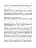
In this figure, there are three graphs. The first one shows the spatial correlation function
between two isotropic radiators, without mutual coupling; The second one presents two
dipoles without mutual coupling; and third plot shows the correlation between two real
dipoles taking into account mutual coupling. The first case of isotropic radiators, shows a
sinc shape, which corresponds to the well known theoretical studies. For dipole antennas,
which were not taken into account the mutual coupling, the plot is nearly a sinc. The
changes are due the radiation pattern of dipoles are not isotropic, but toroidal, with zones
with high radiation and zones where the radiation is entirely null. The plot does not reach
the minimum at zero or negative but the general shape of the graph is still approaching the
sinc. The third plot is linked to the situation of coupled dipoles, is the real case and the
explanation of how they are less defined exponentially decreasing is in two fundamental
reasons: The first is that the radiators are not isotropic, as explained in the previous
situation; the second is that when taking into account the mutual coupling, radiation
patterns of the two dipoles are changing because of the electromagnetic interaction between
them to vary the separation, so changing the directivity
Max
D , the radiation resistance
Rad
R
of both dipoles, and their effective lengths
Ef
l (14). The computations have been performed
using a sampled radiation pattern matrix of dimension of 360 x 180. This matrix can include
not only simulated values but measured patterns providing an early measurement of the
correlation coefficients. Moreover it can evaluate systems built without having to measure
them in a reverberation chamber with problems that this implies (time, complexity of the
measures, special tools, etc).
4. Radio channels classification
Experience has shown that information about their average values is not sufficient to ensure
the quality of performance of radio-communications systems, which takes into account a
ElectrodynamicAnalysisofAntennasinMultipathConditions 447
An important outcome of the simulation is the fact that the signal statistics obtained
corresponds closely to real signal channels (Blaunstein et al., 2002). This also provides an
explanation of the operation of the receiving antennas under multipath environments, the
idea can be reused for practical purposes. So, it is possible the measurement of spatial
correlation in systems multi-antennas, as Kildal & Rosengren (2002) has proposed to
evaluate the performance of. The evaluation of multi-antennas systems from the point of
view of their spatial correlation is based on the implementation of the virtual radio channel
which interact between various antennas simultaneously. The correlation between the
envelopes of the induced e.m f. between the different antennas is calculated including the
interaction with the virtual radio channel. Measured of the radiation patterns of the different
antennas are obtained in an anechoic chamber, or they are simulated by means of
electromagnetic simulation. It’s important to emphasize that it takes into account the mutual
coupling between antennas, which are implicit in the tabulated measured of the radiation
characteristics (radiation patterns of antennas, directivity, and radiation resistance). The
equation of the correlation coefficient between the envelopes associated with the signal
terminals of any two antennas of the system is as follows (Hill, 2002):
22
tsts
tsts
BA
BA
[V]
(33)
Figure 14 shows the problem of evaluation is a system of two separate and parallel dipoles,
please note that both measures are related to the origin of the same coordinate system.
Fig. 14. Geometry of the problem with two antennas under test.
As an example the spatial correlation coefficient as a function of separation between the
electric dipoles has been computed and the obtained results are shown in Figure 15.
0 0.1 0.2 0.3 0.4 0.5 0.6 0.7 0.8 0.9 1
-0.4
-0.2
0
0.2
0.4
0.6
0.8
1
electrical spacing
Correlation
isotropic radiator
not coupled dipoles
coupled dipoles
Fig. 15. Correlation coefficients as a function of spatial separation between antenna
elements.
In this figure, there are three graphs. The first one shows the spatial correlation function
between two isotropic radiators, without mutual coupling; The second one presents two
dipoles without mutual coupling; and third plot shows the correlation between two real
dipoles taking into account mutual coupling. The first case of isotropic radiators, shows a
sinc shape, which corresponds to the well known theoretical studies. For dipole antennas,
which were not taken into account the mutual coupling, the plot is nearly a sinc. The
changes are due the radiation pattern of dipoles are not isotropic, but toroidal, with zones
with high radiation and zones where the radiation is entirely null. The plot does not reach
the minimum at zero or negative but the general shape of the graph is still approaching the
sinc. The third plot is linked to the situation of coupled dipoles, is the real case and the
explanation of how they are less defined exponentially decreasing is in two fundamental
reasons: The first is that the radiators are not isotropic, as explained in the previous
situation; the second is that when taking into account the mutual coupling, radiation
patterns of the two dipoles are changing because of the electromagnetic interaction between
them to vary the separation, so changing the directivity
Max
D , the radiation resistance
Rad
R
of both dipoles, and their effective lengths
Ef
l (14). The computations have been performed
using a sampled radiation pattern matrix of dimension of 360 x 180. This matrix can include
not only simulated values but measured patterns providing an early measurement of the
correlation coefficients. Moreover it can evaluate systems built without having to measure
them in a reverberation chamber with problems that this implies (time, complexity of the
measures, special tools, etc).
4. Radio channels classification
Experience has shown that information about their average values is not sufficient to ensure
the quality of performance of radio-communications systems, which takes into account a
AdvancedMicrowaveandMillimeterWave
Technologies:SemiconductorDevices,CircuitsandSystems448
number of parameters of great importance to the design, operates and manage the radio
system. Moreover, some concepts have been used in the previous sections but they need
deep explanations :
Fading is the sudden variation and reduction of signal received power with respect to its
nominal value. This is due to the superposition of waves that arrive by different path. The
phenomenon has a basically spatial nature, but the spatial variations of the signal are
experienced as temporal variations when the receiver or transmitter they move through the
dispersive channel. Figure.16 shows the parameters of the interest for the signal
characterization, as: the nominal power received
dBmP
N
, the depth of the fading
dBmP
F
,
and the duration of the fading
.
Fig. 16. Fading parameters
Fading performances produces changes in the the spectral characteristics, probability
distributions of radio channel. Table 1 shows a classification according to the fading
parameters according to the mentioned parameters.
Characteristics Fading Type
Depth Deep Very Deep
Duration slow Fast
Spectral characteristics flat Selective
Generating mechanism k factor Multipath
Probability distribution Gaussian Rayleigh, Rice
Table 1. Fading classification
Table 1, provides various kinds of fading in two columns, within which there is some
relationships. Deep fade is usually selective and caused by multipath interference. A flat
fading plane appears normally in case of narrow bandwidth producing the same distortion
along the carrier spectrum. On the other hand, the selective fading produces different
distortions along the spectrum of the modulated signal. Time variation of the desired signal
and interference, plays a crucial role in the reliability analysis of a system imposing
requirements to the type of modulation, transmission power, protection ratio against
interference, diversity techniques, and coding method. That is why; output signal from a
radio channel is studied as a random process using statistical methods to characterize them.
The radio channels are classified taking the name of the statistical distribution function that
describes the signal obtained. In this way, some typical channels are: Normal, Gaussian,
Rayleigh, Rice, and Nakagami. In the case of the fading signals at the terminals of the antennas
that operate under multipath, Practice has shown that the probability distributions that best
fit are: Rayleigh, and Nakagami-Rice. Then will analyze these distributions (Rec. ITU-R P.
1057-1, 2001).
Rayleigh, when several multipath components with an angle of arrival that are uniformly
distributed in the in the range
20
, the Rayleigh distribution describes the fading fast of
the signal envelope, both spatial and temporal. Therefore, it can be obtained mathematically
as envelope limit of the sum of two noise signals in quadrature with Gaussians
distributions. The probability density function, PDF, is expressed as follows:
00
0
2
exp
2
2
2
x
x
xx
(34)
Equation (34),
x
is the random variable and
2
variance or average voltage of the envelope
of the received signal. Its maximum value is
/6065.05.0exp and it corresponds to
the random variable
x
. The cumulative distribution function CDF which is given by:
X
X
dxxPDFXxCDF
0
2
2
2
exp1Pr
(35)
The average value
mean
x of the Rayleigh distribution can be obtained from the condition:
0
253.1
2
dxxPDFxx
mean
(36)
while the variance or average power of the signal envelope of the Rayleigh distribution can
be determined as:
22
2
0
22
429.0
2
2
2
dxxPDFx
x
(37)
The
rms
value of the envelope signal is defined by the square root of
2
2
, is :
414.12rms
(38)
The median of the envelope of this signal is defined from the following condition:
median
x
dxxPDF
0
2
1
(39)
ElectrodynamicAnalysisofAntennasinMultipathConditions 449
number of parameters of great importance to the design, operates and manage the radio
system. Moreover, some concepts have been used in the previous sections but they need
deep explanations :
Fading is the sudden variation and reduction of signal received power with respect to its
nominal value. This is due to the superposition of waves that arrive by different path. The
phenomenon has a basically spatial nature, but the spatial variations of the signal are
experienced as temporal variations when the receiver or transmitter they move through the
dispersive channel. Figure.16 shows the parameters of the interest for the signal
characterization, as: the nominal power received
dBmP
N
, the depth of the fading
dBmP
F
,
and the duration of the fading
.
Fig. 16. Fading parameters
Fading performances produces changes in the the spectral characteristics, probability
distributions of radio channel. Table 1 shows a classification according to the fading
parameters according to the mentioned parameters.
Characteristics Fading Type
Depth Deep Very Deep
Duration slow Fast
Spectral characteristics flat Selective
Generating mechanism k factor Multipath
Probability distribution Gaussian Rayleigh, Rice
Table 1. Fading classification
Table 1, provides various kinds of fading in two columns, within which there is some
relationships. Deep fade is usually selective and caused by multipath interference. A flat
fading plane appears normally in case of narrow bandwidth producing the same distortion
along the carrier spectrum. On the other hand, the selective fading produces different
distortions along the spectrum of the modulated signal. Time variation of the desired signal
and interference, plays a crucial role in the reliability analysis of a system imposing
requirements to the type of modulation, transmission power, protection ratio against
interference, diversity techniques, and coding method. That is why; output signal from a
radio channel is studied as a random process using statistical methods to characterize them.
The radio channels are classified taking the name of the statistical distribution function that
describes the signal obtained. In this way, some typical channels are: Normal, Gaussian,
Rayleigh, Rice, and Nakagami. In the case of the fading signals at the terminals of the antennas
that operate under multipath, Practice has shown that the probability distributions that best
fit are: Rayleigh, and Nakagami-Rice. Then will analyze these distributions (Rec. ITU-R P.
1057-1, 2001).
Rayleigh, when several multipath components with an angle of arrival that are uniformly
distributed in the in the range
20
, the Rayleigh distribution describes the fading fast of
the signal envelope, both spatial and temporal. Therefore, it can be obtained mathematically
as envelope limit of the sum of two noise signals in quadrature with Gaussians
distributions. The probability density function, PDF, is expressed as follows:
00
0
2
exp
2
2
2
x
x
xx
(34)
Equation (34),
x
is the random variable and
2
variance or average voltage of the envelope
of the received signal. Its maximum value is
/6065.05.0exp and it corresponds to
the random variable
x
. The cumulative distribution function CDF which is given by:
X
X
dxxPDFXxCDF
0
2
2
2
exp1Pr
(35)
The average value
mean
x of the Rayleigh distribution can be obtained from the condition:
0
253.1
2
dxxPDFxx
mean
(36)
while the variance or average power of the signal envelope of the Rayleigh distribution can
be determined as:
22
2
0
22
429.0
2
2
2
dxxPDFx
x
(37)
The
rms
value of the envelope signal is defined by the square root of
2
2
, is :
414.12rms
(38)
The median of the envelope of this signal is defined from the following condition:
median
x
dxxPDF
0
2
1
(39)
AdvancedMicrowaveandMillimeterWave
Technologies:SemiconductorDevices,CircuitsandSystems450
and it is obtained:
177.1
median
x
(40)
All these parameters are presented in the x-axis of Figure 17.
Rice distribution appears when several multipath components and a line of sight component
are added between the antennas of the transmitter and receiver. A parameter, known as
K
factor, is introduced, which is the rate between the following components:
componentsmultipath theofPower
componentdominant theofPower
K
(41)
Usually, the PDF and CDF functions of this distribution are expressed in terms of the
K
factor, as shown:
K
x
IK
xx
xPDF 2exp
2
exp
0
2
2
2
(42)
and
0
2
2
2
2
2
exp1
m
m
m
K
x
I
x
Kx
KxCDF
(43)
The K factor is represented by the following ratio
22
2
AK , where
A
is the peak voltage
of the power or envelope of the dominant component,
o
I and
m
I are the modified
Bessel function of first kind and zero order and m respectively. Figure 17 shows the
Rayleigh PDF graph and some PDF graphs of the several
K
values. See in this graph (figure
17a) that is asymmetrical bell-shaped, and that with increasing the
K
value (figure 17b), the
graphics are changing so. In the case where
0K
, the Rice distribution becomes a Rayleigh
distribution, this is perfectly understandable, because for this value is not presence of
dominant component of signal, and is only in the presence of multipath components. When
K
is increasing the graphics are starting to be tighten and tend to a Gaussian distribution.
This is a result of the increase in signal level associated with the dominant component. This
is the real situation when exist the line-of-sight between the antennas of the transmitter and
receiver.
0 0.5 1 1.5 2 2.5 3
0
0.1
0.2
0.3
0.4
0.5
0.6
0.7
0.8
x
(a)
PDF(x)
0 0.5 1 1.5 2 2.5 3
0
0.5
1
1.5
2
2.5
3
3.5
V rms (V)
(b)
PDF(x)
K=0
K=4
K=16
K=32
Rayleigh
Rayleigh
Fig. 17. a) Rayleigh density function and b) Rayleigh PDF for the several
K
values
In practice usually identified mixed distributions. Identification of the type given channel
fluctuations at the terminals of an antenna probe is of great importance. Knowledge of the
channel parameters associated allows selecting the most suitable antenna system, both in the
transmitter as the receiver system, allows the configuration of the all signal processing.
Knowing the parameter of the channel allow to define the all the structure of the radio
system.
5. Conclusions
In this chapter an analysis on the behaviour of antennas in the reception system has been
performed. The conclusions are the basis for the approach to the problem of antennas in
receiving mode operating in multipath conditions. It was shown that many properties of the
antennas are the same in transmission and in reception, which simplifies its study, since it is
not necessary to determine these properties in both regimes. Thus, the impedance of the
antenna, directional properties, its directivity, efficiency, and gain are the same in both ways
of work. Several expressions (mainly the induced e.m.f), at the receiving antenna has been
obtained. An analysis of the flow of electromagnetic power from the wave travelling in free
space and incident at the antenna until you arrive to the receiver, several causes of loss that
can occur in this tract were shown, allowing to define conditions to be met to achieve
optimal reception: coincidence of the polarization of the antenna with of the incident wave,
orientation of the antenna with the direction of arrival of the wave, maximum effective area
antenna (length), which depends on its building characteristics, high efficiency, impedances
matching between the antenna and feed line. Once the theory and basis on the antenna in
reception mode has been stated, the operation under multipath conditions has been covered.
A computational procedure that allows see the behaviour an antenna when waves impinge
from all directions of space has been presented. The presented procedure has been proved to
be useful not only from an educational point of view, but also for assessment multi-antennas
system from the viewpoint of spatial correlation, which generalizes its range of applicability.
Finally, the importance of classification and identification of radio channels has been
explained through a statistical analysis of the fading signal at its terminals. Rice and Rayleigh
channels models were used that best describe the main essence of the multipath. It was
observed that when decreasing the signal level of the dominant path this one tends to
Rayleigh. Knowing the behaviour of antennas under multipath conditions is of significant
ElectrodynamicAnalysisofAntennasinMultipathConditions 451
and it is obtained:
177.1
median
x
(40)
All these parameters are presented in the x-axis of Figure 17.
Rice distribution appears when several multipath components and a line of sight component
are added between the antennas of the transmitter and receiver. A parameter, known as
K
factor, is introduced, which is the rate between the following components:
componentsmultipath theofPower
componentdominant theofPower
K
(41)
Usually, the PDF and CDF functions of this distribution are expressed in terms of the
K
factor, as shown:
K
x
IK
xx
xPDF 2exp
2
exp
0
2
2
2
(42)
and
0
2
2
2
2
2
exp1
m
m
m
K
x
I
x
Kx
KxCDF
(43)
The K factor is represented by the following ratio
22
2
AK , where
A
is the peak voltage
of the power or envelope of the dominant component,
o
I and
m
I are the modified
Bessel function of first kind and zero order and m respectively. Figure 17 shows the
Rayleigh PDF graph and some PDF graphs of the several
K
values. See in this graph (figure
17a) that is asymmetrical bell-shaped, and that with increasing the
K
value (figure 17b), the
graphics are changing so. In the case where
0K
, the Rice distribution becomes a Rayleigh
distribution, this is perfectly understandable, because for this value is not presence of
dominant component of signal, and is only in the presence of multipath components. When
K
is increasing the graphics are starting to be tighten and tend to a Gaussian distribution.
This is a result of the increase in signal level associated with the dominant component. This
is the real situation when exist the line-of-sight between the antennas of the transmitter and
receiver.
0 0.5 1 1.5 2 2.5 3
0
0.1
0.2
0.3
0.4
0.5
0.6
0.7
0.8
x
(a)
PDF(x)
0 0.5 1 1.5 2 2.5 3
0
0.5
1
1.5
2
2.5
3
3.5
V rms (V)
(b)
PDF(x)
K=0
K=4
K=16
K=32
Rayleigh
Rayleigh
Fig. 17. a) Rayleigh density function and b) Rayleigh PDF for the several
K
values
In practice usually identified mixed distributions. Identification of the type given channel
fluctuations at the terminals of an antenna probe is of great importance. Knowledge of the
channel parameters associated allows selecting the most suitable antenna system, both in the
transmitter as the receiver system, allows the configuration of the all signal processing.
Knowing the parameter of the channel allow to define the all the structure of the radio
system.
5. Conclusions
In this chapter an analysis on the behaviour of antennas in the reception system has been
performed. The conclusions are the basis for the approach to the problem of antennas in
receiving mode operating in multipath conditions. It was shown that many properties of the
antennas are the same in transmission and in reception, which simplifies its study, since it is
not necessary to determine these properties in both regimes. Thus, the impedance of the
antenna, directional properties, its directivity, efficiency, and gain are the same in both ways
of work. Several expressions (mainly the induced e.m.f), at the receiving antenna has been
obtained. An analysis of the flow of electromagnetic power from the wave travelling in free
space and incident at the antenna until you arrive to the receiver, several causes of loss that
can occur in this tract were shown, allowing to define conditions to be met to achieve
optimal reception: coincidence of the polarization of the antenna with of the incident wave,
orientation of the antenna with the direction of arrival of the wave, maximum effective area
antenna (length), which depends on its building characteristics, high efficiency, impedances
matching between the antenna and feed line. Once the theory and basis on the antenna in
reception mode has been stated, the operation under multipath conditions has been covered.
A computational procedure that allows see the behaviour an antenna when waves impinge
from all directions of space has been presented. The presented procedure has been proved to
be useful not only from an educational point of view, but also for assessment multi-antennas
system from the viewpoint of spatial correlation, which generalizes its range of applicability.
Finally, the importance of classification and identification of radio channels has been
explained through a statistical analysis of the fading signal at its terminals. Rice and Rayleigh
channels models were used that best describe the main essence of the multipath. It was
observed that when decreasing the signal level of the dominant path this one tends to
Rayleigh. Knowing the behaviour of antennas under multipath conditions is of significant
AdvancedMicrowaveandMillimeterWave
Technologies:SemiconductorDevices,CircuitsandSystems452
importance to the engineers who design, plan and operate radio systems, in order to
configure, optimize and select proper system elements, which are ultimately defined by the
set-antenna channel.
6. References
Balanis, C. A. (1982). Antennas Theory: analysis and design, Edit. Harper & Row, ISBN 0-471-
59268-4, New Jersey
Blaunstein, N & Andersen, J. B. (2002). Multipath Phenomena in Cellular Network, Edit.
Hartech House Inc, ISBN-158053-185-7, New York
Hill, D. A & Ladbury, J. M. (2003). Spatial-Correlation Functions of Fields and Energy
Density in a Reverberation Chamber, IEEE Transaction on electromagnetic
compatibility, Vol.44, No. 1. , February 2002. pp. 95-101, ISSN 0018-9375
Kildal, P-S & Rosengren, K. (2003). Electromagnetic analysis of effective and apparent
diversity gain of two parallel, IEEE Antennas and Wireless Propagation Letters, Vol. 2,
No. 1, pp 9-13, ISSN 1536-1225
Ludwig, A.C. (1973). The Definition of Cross Polarization. IEEE Transaction on Antennas and
Propagation, pp. 116-119, Jan 1973
Márkov, G.T. & Sazónov, D. M. (1978). Antenas. Edit. MIR, ISBN 9785884170797, URSS
Molina, E. L & De Haro, L. A. (2007). Antenna and Wireless Multipath Virtual Channel
Interaction, Proceedings of IEEE-MTT, pp. 1-3, ISBN 978-1-4244-0748-4, December
2007, Bangkok
Molina, E. L & De Haro, L. A. (2008). Statistical characterization of the antenna and wireless
multipath virtual channel interaction, Proceedings of IEEE-APS, pp. 1-4, ISBN 978-
1-4244-2041-4, September 2008, San Diego. CA
Monson, J.C. (1996). A new reciprocity theorem, IEEE Transaction on Antennas and
Propagation, Vol.44, No. 1. , February 1996. pp. 10-14, ISSN 0018-9480
Nikolski, V. V. (1976). Electrodinámica y propagación de las ondas de radio, Edit. URSS, ISBN-
9785884170551, Moscú
Rec. ITU-R P. 1057-1 (2001), Probability distributions relevant to radiowave propagation
modelling, Edit. ITU
Rogier, H. (2006). Phase-mode construction of a coupling matrix for uniform circular arrays
with a center element, Microwave Optical Technology Letters, Vol. 48, No. 2, February
2006. pp. 291-298, ISSN 0895-2477
FoamedNanocompositesforEMIShieldingApplications 453
FoamedNanocompositesforEMIShieldingApplications
IsabelMolenberg,IsabelleHuynen,Anne-ChristineBaudouin,ChristianBailly,Jean-Michel
ThomassinandChristopheDetrembleur
x
Foamed Nanocomposites for EMI
Shielding Applications
Isabel Molenberg, Isabelle Huynen, Anne-Christine Baudouin, Christian
Bailly, Jean-Michel Thomassin and Christophe Detrembleur
Université Catholique de Louvain, Université de Liège
Belgium
1. Introduction
The addition of nanoparticles having specific properties inside a matrix with different
properties creates a novel material that exhibits hybrid and even new properties. The
nanocomposites presented in this paper combine the properties of foamed polymers
(inexpensive, lightweight, easy to mould into any desired shape, etc.) with those of carbon
nanotubes (CNTs). The addition of any conductive nanoparticles to an otherwise insulating
matrix leads to a significant increase of the electrical conductivity. But CNTs have a very
high aspect ratio; a much lower content of CNTs is therefore required to get the same
conductivity increase as the one obtained with more compact nanoparticles.
This is especially interesting for EMI shielding materials since, as will be explained in
further details in this chapter, it is desirable for such materials to have a high conductivity
but a low dielectric constant, in order to minimize the electromagnetic power outside the
shield casing but also to minimize the power reflected back inside the casing, as is explained
in section 2. In particular, two parameters of interest when comparing shielding materials
are detailed and discussed.
The polymer/CNTs nanocomposites were fabricated and characterized using a two-step
diagnostic method. They were first characterized in their solid form, i.e. before the foaming
process and the most interesting polymer matrices (with embedded CNTs) could be
selected. This way, only the promising blends were foamed, therefore avoiding the
unnecessary fabrication of a number of foams. These selected blends were foamed and then
characterized. The samples, both solid and foamed, are described and their fabrication
processes are briefly explained in section 3 while the characterization methods are shown in
section 4.
A simple electrical model is given and explained in section 5 and an optimized topology for
the foams is also proposed in the second part of the same section.
The measurement results for the solids and for the mono-layered and multi-layered foams
are summarized and discussed in section 6. They are then compared to results obtained
using the electrical model presented in the previous section and they are also correlated to
rheological characterizations.
23
AdvancedMicrowaveandMillimeterWave
Technologies:SemiconductorDevices,CircuitsandSystems454
2. EMI shielding considerations
There are two main parameters that are used to characterize the quality of a shielding
material in terms of electromagnetic power; the Shielding Effectiveness (SE) and the
Reflectivity (R). The former relates the power that is transmitted through the material (P
out
),
cf. Fig. 1(left), to the incident power (P
in
): SE = 10 log (P
in
/P
out
). The latter relates the power
reflected back from the material (P
ref
) to the incident power (P
in
): R=10 log(P
ref
/P
in
).
The incident power is either reflected back, or transmitted through the material to the outer
world, or absorbed inside the material, P
in
= P
ref
+ P
out
+ A
2
, where A
2
is the power absorbed
inside the material. A is called the attenuation and increases as the conductivity of the
material increases. The power reflected at the interface air-material is higher when the
difference between the dielectric constants on both sides of the interface is more important.
Since air has a dielectric constant of 1, the Reflectivity increases with the dielectric constant
of the shielding material.
It must be noted that the above discussion does not take into account the reflection at the
second interface, material to air. To be exact we should consider this extra reflection but its
effect becomes negligible when the attenuation is sufficiently high, cf. (Huynen et al., 2008).
It is not always enough for a shielding material to exhibit a good SE, i.e. stopping power
transmission to the outside world. For example, metallic materials have a high SE at high
frequency but almost all the incident power is reflected back inside the shield casing (high
R), possibly interfering with other inner elements (or even with the emitter itself). Materials
that combine a high SE with a low R at microwave frequencies are called microwave
absorbers, because the power is absorbed inside the material, cf. Fig. 1(right). For a material
to have a high SE, it must exhibit a high conductivity and, in order to have a low R, it must
have a low dielectric constant.
Fig. 1. Schematic diagrams for a conventional metallic shielding material (left) and for a
microwave absorber (right).
Finding a material that combines a high electrical conductivity and a low dielectric constant
is not trivial. This is the idea behind the use of foamed nanocomposites. In theory, foaming a
material would decrease its dielectric constant (because of the porosity and because air has
dielectric constant of 1). On the other hand, the addition of conductive nanoparticles to a
material should theoretically increase its conductivity, cf. (Huynen et al., 2008), (Thomassin
et al., 2008).
Besides having a potentially low dielectric constant, polymer foams are inexpensive,
lightweight and easy to mould into any desirable shape. And, the addition of conductive
nanoparticles would also reinforce the polymer matrix, improving its electrical conductivity
but also its mechanical properties and its thermal conductivity, cf. (Saib et al. 2006). Carbon
nanotubes have a very high aspect-ratio (≥1000). They can therefore form extensive regular
conductive networks with a much lower content than other nanoparticles having a more
spherical or compact shape, cf. Fig. 2.
20 25 30 35 40
0
5
10
15
Attenuation[dB]
Frequency(GHz)
CNT0.5%
CB5%
Fig. 2. Influence of the type of nanoparticles, CBs or CNTs, on the attenuation of a
nanocomposite, from (Saib et al. 2006).
The applications of such foamed nanocomposites are numerous and varied, from electronics
packaging to bioneural matrices, in aeronautics, automotive, environmental applications,
and many more
But the most promising application at the moment is certainly as shielding materials, more
precisely as microwave absorbers. They could be made into thin, large, flexible, lightweight
panels to be used as EMI shielding materials anywhere, and for little cost. Those panels
could also have interesting fire retardancy or protection again electrostatic discharges
properties.
3. Nanocomposite samples description
The chemical processes involved in the fabrication of foamed samples are rather complex, cf.
section 3.2 for more details. It is therefore interesting to make a first selection on the
nanocomposite blends before they are actually foamed. A two-step diagnostic method was
developed; solid samples of polymer-CNTs blends were first characterized (the so-called
screening tests), the best candidate blends were then used to fabricate foams and finally the
foamed samples were also characterized.
3.1 Solid thin-film samples (screening tests)
The CNTs used for the fabrication of the nanocomposites are commercially available thin
MultiWalled NanoTubes (MWNTs), with an average outer diameter of 10 nm and a purity
over 95%. They were produced using Catalytic Carbon Vapour Deposition (CCVD) by
Nanocyl SA (Belgium).
FoamedNanocompositesforEMIShieldingApplications 455
2. EMI shielding considerations
There are two main parameters that are used to characterize the quality of a shielding
material in terms of electromagnetic power; the Shielding Effectiveness (SE) and the
Reflectivity (R). The former relates the power that is transmitted through the material (P
out
),
cf. Fig. 1(left), to the incident power (P
in
): SE = 10 log (P
in
/P
out
). The latter relates the power
reflected back from the material (P
ref
) to the incident power (P
in
): R=10 log(P
ref
/P
in
).
The incident power is either reflected back, or transmitted through the material to the outer
world, or absorbed inside the material, P
in
= P
ref
+ P
out
+ A
2
, where A
2
is the power absorbed
inside the material. A is called the attenuation and increases as the conductivity of the
material increases. The power reflected at the interface air-material is higher when the
difference between the dielectric constants on both sides of the interface is more important.
Since air has a dielectric constant of 1, the Reflectivity increases with the dielectric constant
of the shielding material.
It must be noted that the above discussion does not take into account the reflection at the
second interface, material to air. To be exact we should consider this extra reflection but its
effect becomes negligible when the attenuation is sufficiently high, cf. (Huynen et al., 2008).
It is not always enough for a shielding material to exhibit a good SE, i.e. stopping power
transmission to the outside world. For example, metallic materials have a high SE at high
frequency but almost all the incident power is reflected back inside the shield casing (high
R), possibly interfering with other inner elements (or even with the emitter itself). Materials
that combine a high SE with a low R at microwave frequencies are called microwave
absorbers, because the power is absorbed inside the material, cf. Fig. 1(right). For a material
to have a high SE, it must exhibit a high conductivity and, in order to have a low R, it must
have a low dielectric constant.
Fig. 1. Schematic diagrams for a conventional metallic shielding material (left) and for a
microwave absorber (right).
Finding a material that combines a high electrical conductivity and a low dielectric constant
is not trivial. This is the idea behind the use of foamed nanocomposites. In theory, foaming a
material would decrease its dielectric constant (because of the porosity and because air has
dielectric constant of 1). On the other hand, the addition of conductive nanoparticles to a
material should theoretically increase its conductivity, cf. (Huynen et al., 2008), (Thomassin
et al., 2008).
Besides having a potentially low dielectric constant, polymer foams are inexpensive,
lightweight and easy to mould into any desirable shape. And, the addition of conductive
nanoparticles would also reinforce the polymer matrix, improving its electrical conductivity
but also its mechanical properties and its thermal conductivity, cf. (Saib et al. 2006). Carbon
nanotubes have a very high aspect-ratio (≥1000). They can therefore form extensive regular
conductive networks with a much lower content than other nanoparticles having a more
spherical or compact shape, cf. Fig. 2.
20 25 30 35 40
0
5
10
15
Attenuation[dB]
Frequency(GHz)
CNT0.5%
CB5%
Fig. 2. Influence of the type of nanoparticles, CBs or CNTs, on the attenuation of a
nanocomposite, from (Saib et al. 2006).
The applications of such foamed nanocomposites are numerous and varied, from electronics
packaging to bioneural matrices, in aeronautics, automotive, environmental applications,
and many more
But the most promising application at the moment is certainly as shielding materials, more
precisely as microwave absorbers. They could be made into thin, large, flexible, lightweight
panels to be used as EMI shielding materials anywhere, and for little cost. Those panels
could also have interesting fire retardancy or protection again electrostatic discharges
properties.
3. Nanocomposite samples description
The chemical processes involved in the fabrication of foamed samples are rather complex, cf.
section 3.2 for more details. It is therefore interesting to make a first selection on the
nanocomposite blends before they are actually foamed. A two-step diagnostic method was
developed; solid samples of polymer-CNTs blends were first characterized (the so-called
screening tests), the best candidate blends were then used to fabricate foams and finally the
foamed samples were also characterized.
3.1 Solid thin-film samples (screening tests)
The CNTs used for the fabrication of the nanocomposites are commercially available thin
MultiWalled NanoTubes (MWNTs), with an average outer diameter of 10 nm and a purity
over 95%. They were produced using Catalytic Carbon Vapour Deposition (CCVD) by
Nanocyl SA (Belgium).