Advances in Robot Manipulators Part 17 ppt
Bạn đang xem bản rút gọn của tài liệu. Xem và tải ngay bản đầy đủ của tài liệu tại đây (909 KB, 40 trang )
AdvancesinRobotManipulators632
Similar to the those established in (De Silva, 1976; Sooraksa & Chen, 1998), equation (16) is
the fifth order TB homogeneous linear PDE with internal and external damping effects
expressing the deflection
( , )w x t
.
We have added to this equation the following initial and pinned (clamped)-mass boundary
conditions (Loudini et al., 2007a, Loudini et al., 2006):
UInitial conditions:U
0
( ,0)w x w ,
0
0
( , )
t
w x t
w
t
(18)
UPinned end:U (0, ) 0w t ,
3
2
0
( , )
( , ) 0
h
x
w x t
M x t J
x t
(19)
UClamped end:U (0, ) 0w t ,
0
( , )
0
x
w x t
x
(20)
UFree end with payload mass:U
2
2
3
2
( , ) ( , )
0
( , )
( , ) 0
p
x
p
x
M x t w x t
M
x t
w x t
M x t J
x t
(21)
The classical fourth order TB PDE is retrieved if the damping effects terms are suppressed:
4 4 2 4 2
4 2 2 4 2
( , ) ( , ) ( , ) ( , )
1 0
w x t E w x t ρ I w x t w x t
EI ρI ρA
x KG x t KG t t
(22)
If the effect due to the rotary inertia is neglected, we are led to the shear beam (SB) model
(Morris, 1996; Han et al., 1999):
4 4 2
4 2 2 2
( , ) ( , ) ( , )
0
w x t ρIE w x t w x t
EI ρA
x KG x t t
(23)
but, if the one due to shear distortion is the neglected one, the Rayleigh beam equation (Han
et al., 1999; Rayleigh, 2003) arises:
4 4 2
4 2 2 2
( , ) ( , ) ( , )
0
w x t w x t w x t
EI ρI ρA
x x t t
(24)
Moreover, if both the rotary inertia and shear deformation are neglected, then the governing
equation of motion reduces to that based on the classical EBT (Meirovitch, 1986) given by
4 2
4 2
( , ) ( , )
0
w x t w x t
EI ρA
x t
(25)
If the above included damping effects are associated to the EBB, the corresponding PDE is
5 4 2
4 4 2
( , ) ( , ) ( , ) ( , )
0
D D
w x t w x t w x t w x t
K I EI ρA A
x t x t t
(26)
The resolution of the PDE with mixed derivative terms (16) is a complex mathematical
problem. Among the few methods existing in the literature, we cite the following
approaches with some representative works: the finite element method (Kapur, 1966; Hoa,
1979; Kolberg 1987), the Galerkin method (Wang and Chou, 1998; Dadfarnia et al., 2005), the
Rayleigh-Ritz method (Oguamanam and Heppler, 1996), the Laplace transform method
resulting in an integral form solution (Boley & Chao, 1955; Wang & Guan, 1994; Ortner &
Wagner, 1996), and the eigenfunction expansion method, also referred to as the series or
modal expansion method (Anderson, 1953; Dolph, 1954; Huang, 1961; Ekwaro-Osire et al.,
2001; Loudini et al. 2006; Loudini et al. 2007a; Loudini et al. 2007b).
In the latter one,
( , )w x t can take the following expanded separated form which consists of
an infinite sum of products between the chosen transverse deflection eigenfunctions or
mode shapes
( )
n
W x , that must satisfy the pinned (clamped)-free (mass) BCs, and the time-
dependant modal generalized coordinates
( )
n
δ t
:
1
( , ) ( ) ( )
n n
n
w x t W x δ t
(27)
2.4 Dynamic model deriving procedure
In order to obtain a set of ordinary differential equations (ODEs) of motion to adequately
describe the dynamics of the flexible link manipulator, the Hamilton's or Lagrange's
approach combined with the Assumed Modes Method (AMM) (Fraser & Daniel, 1991;
Loudini et al. 2006; Loudini et al. 2007a; Loudini et al. 2007b; Tokhi & Azad, 2008) can be
used.
According to the Lagrange's method, a dynamic system completely located by
n
generalized coordinates
i
q must satisfy
n
differential equations of the form:
i
i i i
d L L D
F
dt q q q
,
0,1,2,i
(28)
where
L is the so-called Lagrangian given by
L T U
(29)
TimoshenkoBeamTheorybasedDynamicModeling
ofLightweightFlexibleLinkRoboticManipulators 633
Similar to the those established in (De Silva, 1976; Sooraksa & Chen, 1998), equation (16) is
the fifth order TB homogeneous linear PDE with internal and external damping effects
expressing the deflection
( , )w x t
.
We have added to this equation the following initial and pinned (clamped)-mass boundary
conditions (Loudini et al., 2007a, Loudini et al., 2006):
UInitial conditions:U
0
( ,0)w x w ,
0
0
( , )
t
w x t
w
t
(18)
UPinned end:U (0, ) 0w t
,
3
2
0
( , )
( , ) 0
h
x
w x t
M x t J
x t
(19)
UClamped end:U (0, ) 0w t
,
0
( , )
0
x
w x t
x
(20)
UFree end with payload mass:U
2
2
3
2
( , ) ( , )
0
( , )
( , ) 0
p
x
p
x
M x t w x t
M
x t
w x t
M x t J
x t
(21)
The classical fourth order TB PDE is retrieved if the damping effects terms are suppressed:
4 4 2 4 2
4 2 2 4 2
( , ) ( , ) ( , ) ( , )
1 0
w x t E w x t ρ I w x t w x t
EI ρI ρA
x KG x t KG t t
(22)
If the effect due to the rotary inertia is neglected, we are led to the shear beam (SB) model
(Morris, 1996; Han et al., 1999):
4 4 2
4 2 2 2
( , ) ( , ) ( , )
0
w x t ρIE w x t w x t
EI ρA
x KG x t t
(23)
but, if the one due to shear distortion is the neglected one, the Rayleigh beam equation (Han
et al., 1999; Rayleigh, 2003) arises:
4 4 2
4 2 2 2
( , ) ( , ) ( , )
0
w x t w x t w x t
EI ρI ρA
x x t t
(24)
Moreover, if both the rotary inertia and shear deformation are neglected, then the governing
equation of motion reduces to that based on the classical EBT (Meirovitch, 1986) given by
4 2
4 2
( , ) ( , )
0
w x t w x t
EI ρA
x t
(25)
If the above included damping effects are associated to the EBB, the corresponding PDE is
5 4 2
4 4 2
( , ) ( , ) ( , ) ( , )
0
D D
w x t w x t w x t w x t
K I EI ρA A
x t x t t
(26)
The resolution of the PDE with mixed derivative terms (16) is a complex mathematical
problem. Among the few methods existing in the literature, we cite the following
approaches with some representative works: the finite element method (Kapur, 1966; Hoa,
1979; Kolberg 1987), the Galerkin method (Wang and Chou, 1998; Dadfarnia et al., 2005), the
Rayleigh-Ritz method (Oguamanam and Heppler, 1996), the Laplace transform method
resulting in an integral form solution (Boley & Chao, 1955; Wang & Guan, 1994; Ortner &
Wagner, 1996), and the eigenfunction expansion method, also referred to as the series or
modal expansion method (Anderson, 1953; Dolph, 1954; Huang, 1961; Ekwaro-Osire et al.,
2001; Loudini et al. 2006; Loudini et al. 2007a; Loudini et al. 2007b).
In the latter one,
( , )w x t can take the following expanded separated form which consists of
an infinite sum of products between the chosen transverse deflection eigenfunctions or
mode shapes
( )
n
W x , that must satisfy the pinned (clamped)-free (mass) BCs, and the time-
dependant modal generalized coordinates
( )
n
δ t
:
1
( , ) ( ) ( )
n n
n
w x t W x δ t
(27)
2.4 Dynamic model deriving procedure
In order to obtain a set of ordinary differential equations (ODEs) of motion to adequately
describe the dynamics of the flexible link manipulator, the Hamilton's or Lagrange's
approach combined with the Assumed Modes Method (AMM) (Fraser & Daniel, 1991;
Loudini et al. 2006; Loudini et al. 2007a; Loudini et al. 2007b; Tokhi & Azad, 2008) can be
used.
According to the Lagrange's method, a dynamic system completely located by
n
generalized coordinates
i
q must satisfy
n
differential equations of the form:
i
i i i
d L L D
F
dt q q q
,
0,1,2,i
(28)
where
L is the so-called Lagrangian given by
L T U (29)
AdvancesinRobotManipulators634
T represents the kinetic energy of the modeled system and U its potential energy. Also, in
(28)
D is the Rayleigh's dissipation function which allows dissipative effects to be included,
and
i
F is the generalized external force acting on the corresponding coordinate
i
q .
Theoretically there are infinite number of ODEs, but for practical considerations, such as
boundedness of actuating energy and limitation of the actuators and the sensors working
frequency range, it is more reasonable to truncate this number at a finite one
n
(Cannon &
Schmitz, 1984; Kanoh & Lee, 1985; Qi & Chen, 1992).
The total kinetic energy of the robot flexible link and its potential energy due to the internal
bending moment and the shear force are, respectively, given by (Macchelli & Melchiorri,
2004; Loudini et al. 2006; Loudini et al. 2007a; Loudini et al. 2007b):
2 2
0 0
1 ( , ) 1 ( , )
2 2
w x t γ x t
T
ρ
A dx
ρ
I dx
t t
(30)
2
2
0 0
1 ( , ) 1
( , )
2 2
γ x t
U EI dx KAG σ x t dx
x
(31)
The dissipated energy due to the damping effects can be written as (Krishnan & Vidyasagar,
1988; Loudini et al. 2006; Loudini et al. 2007a; Loudini et al. 2007b):
2
2
3
2
0 0
1 ( , ) 1 ( , )
2 2
D D
w x t w x t
D A dx K I dx
t x t
(32)
Substituting these energies expressions into (28) accordingly and using the transverse
deflection separated form (27), we can derive the desired dynamic equations of motion in
the mass (
B ), damping (
H
), Coriolis and centrifugal forces ( N ) and stiffness (
K
) matrix
familiar form:
2
2
( ) ( )
( ), ( ) ( ) ( )
d q t dq t
B H N q t q t Kq t F t
dt dt
(33)
with
1 2
( ) ( ) ( ) ( ) ( )
T
n
q t θ t δ t δ t δ t
; ( ) 0 0 0
T
F t τ
.
If we disregard some high order and nonlinear terms, under reasonable assumptions, the
matrix differential equation in (33) could be easily represented in a state-space form as
( ) ( ) ( )
( ) ( )
z z
z
z t A z t B u t
y t C z t
(34)
with ( ) 0 0
T
u t τ
;
1 1
( ) ( ) ( ) ( ) ( ) ( ) ( )
T
n n
z t θ t δ t δ t θ t δ t δ t
.
Solving the state-space matrices gives the vector of states
)(tz , that is, the angular
displacement, the modal amplitudes and their velocities.
3. A Special Case Study: Comprehensive Dynamic Modeling of a Flexible
Link Manipulator Considered as a Shear Deformable Timoshenko Beam
In this second part of our work, we present a novel dynamic model of a planar single-link
flexible manipulator considered as a tip mass loaded pinned-free shear deformable beam.
Using the classical TBT described in section 2 and including the Kelvin-Voigt structural
viscoelastic effect (Christensen, 2003), the lightweight robotic manipulator motion
governing PDE is derived. Then, based on the Lagrange's principle combined with the
AMM, a dynamic model suitable for control purposes is established.
3.1 System description and motion governing equation
The considered physical system is shown in Fig. 4. The basic deriving procedure to obtain
the motion governing equation has been described in the previous section, and so only an
outline giving the main steps is presented here.
The effect of rotary inertia being neglected in this case study, equation (10) expressing the
equilibrium of the moments becomes:
( , )
( , )
M x t
S x t
x
(35)
The relation that fellows balancing forces is
2
2
( , ) ( , )S x t w x t
ρA
x t
(36)
Substitution of 6 and 9 into 35 and likewise 6 into 36 yields the two coupled equations of the
damped SB motion:
3 2
2 2
( , ) ( , ) ( , )
( , ) 0
D
γ x t γ x t w x t
K I EI kAG γ x t
x t x x
(37)
2 2
2 2
( , ) ( , ) ( , )
0
w x t γ x t w x t
kAG ρA
x x t
(38)
Equations 37 and 38 can be easily decoupled to obtain the fifth order SB homogeneous linear
PDEs with internal damping effect expressing the deflection
),( txw and the slope of
bending
t),(x
TimoshenkoBeamTheorybasedDynamicModeling
ofLightweightFlexibleLinkRoboticManipulators 635
T represents the kinetic energy of the modeled system and U its potential energy. Also, in
(28)
D is the Rayleigh's dissipation function which allows dissipative effects to be included,
and
i
F is the generalized external force acting on the corresponding coordinate
i
q .
Theoretically there are infinite number of ODEs, but for practical considerations, such as
boundedness of actuating energy and limitation of the actuators and the sensors working
frequency range, it is more reasonable to truncate this number at a finite one
n
(Cannon &
Schmitz, 1984; Kanoh & Lee, 1985; Qi & Chen, 1992).
The total kinetic energy of the robot flexible link and its potential energy due to the internal
bending moment and the shear force are, respectively, given by (Macchelli & Melchiorri,
2004; Loudini et al. 2006; Loudini et al. 2007a; Loudini et al. 2007b):
2 2
0 0
1 ( , ) 1 ( , )
2 2
w x t γ x t
T
ρ
A dx
ρ
I dx
t t
(30)
2
2
0 0
1 ( , ) 1
( , )
2 2
γ x t
U EI dx KAG σ x t dx
x
(31)
The dissipated energy due to the damping effects can be written as (Krishnan & Vidyasagar,
1988; Loudini et al. 2006; Loudini et al. 2007a; Loudini et al. 2007b):
2
2
3
2
0 0
1 ( , ) 1 ( , )
2 2
D D
w x t w x t
D A dx K I dx
t x t
(32)
Substituting these energies expressions into (28) accordingly and using the transverse
deflection separated form (27), we can derive the desired dynamic equations of motion in
the mass (
B ), damping (
H
), Coriolis and centrifugal forces ( N ) and stiffness (
K
) matrix
familiar form:
2
2
( ) ( )
( ), ( ) ( ) ( )
d q t dq t
B H N q t q t Kq t F t
dt dt
(33)
with
1 2
( ) ( ) ( ) ( ) ( )
T
n
q t θ t δ t δ t δ t
; ( ) 0 0 0
T
F t τ
.
If we disregard some high order and nonlinear terms, under reasonable assumptions, the
matrix differential equation in (33) could be easily represented in a state-space form as
( ) ( ) ( )
( ) ( )
z z
z
z t A z t B u t
y t C z t
(34)
with ( ) 0 0
T
u t τ
;
1 1
( ) ( ) ( ) ( ) ( ) ( ) ( )
T
n n
z t θ t δ t δ t θ t δ t δ t
.
Solving the state-space matrices gives the vector of states
)(tz , that is, the angular
displacement, the modal amplitudes and their velocities.
3. A Special Case Study: Comprehensive Dynamic Modeling of a Flexible
Link Manipulator Considered as a Shear Deformable Timoshenko Beam
In this second part of our work, we present a novel dynamic model of a planar single-link
flexible manipulator considered as a tip mass loaded pinned-free shear deformable beam.
Using the classical TBT described in section 2 and including the Kelvin-Voigt structural
viscoelastic effect (Christensen, 2003), the lightweight robotic manipulator motion
governing PDE is derived. Then, based on the Lagrange's principle combined with the
AMM, a dynamic model suitable for control purposes is established.
3.1 System description and motion governing equation
The considered physical system is shown in Fig. 4. The basic deriving procedure to obtain
the motion governing equation has been described in the previous section, and so only an
outline giving the main steps is presented here.
The effect of rotary inertia being neglected in this case study, equation (10) expressing the
equilibrium of the moments becomes:
( , )
( , )
M x t
S x t
x
(35)
The relation that fellows balancing forces is
2
2
( , ) ( , )S x t w x t
ρA
x t
(36)
Substitution of 6 and 9 into 35 and likewise 6 into 36 yields the two coupled equations of the
damped SB motion:
3 2
2 2
( , ) ( , ) ( , )
( , ) 0
D
γ x t γ x t w x t
K I EI kAG γ x t
x t x x
(37)
2 2
2 2
( , ) ( , ) ( , )
0
w x t γ x t w x t
kAG ρA
x x t
(38)
Equations 37 and 38 can be easily decoupled to obtain the fifth order SB homogeneous linear
PDEs with internal damping effect expressing the deflection
),( txw and the slope of
bending
t),(x
AdvancesinRobotManipulators636
5 5 4 4 2
4 2 3 4 2 2 2
( , ) ( , ) ( , ) ( , ) ( , )
0
D
D
w x t ρK I w x t w x t ρEI w x t w x t
K I EI ρA
x t KG x t x KG x t t
(39)
5 5 4 4 2
4 2 3 4 2 2 2
( , ) ( , ) ( , ) ( , ) ( , )
0
D
D
γ x t ρK I γ x t γ x t ρEI γ x t γ x t
K I EI ρA
x t KG x t x KG x t t
(40)
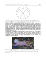
Fig. 4. Physical configuration and kinematics of deformation of a bending element of the
studied flexible robot manipulator considered as a shear deformable beam
0
X
X
0
x
x
0
y
y
),,,(
IE
),( txw
Y
)(t
)(t
Deflected link
Rigid hub (J
h
)
0
Z
0
Y
Beam element
0
X
Center of mass
0
Y
),( tx
Tip payload ),(
pp
JM
dx
x
S
txS
),(
dx
x
M
txM
),(
),( txS
),( txM
2
2
),(
t
txw
A
dx
x dx
x
x
w
X
Y
We affect to the equation (39) the same initial and pinned-mass boundary conditions, given
by equations 18, 19, and 21, with taking into account the result established by (Wang &
Guan, 1994; Loudini et al., 2007b) about the very small influence of the tip payload inertia on
the flexible manipulator dynamics:
UInitial conditions:U
0
( ,0)w x w
,
0
0
( , )
t
t
w x t w
(41)
UBCs at the pinned end (root of the link):
0
( , ) 0
x
w x t
: zero average translational displacement (42)
3
2
0
0
( , )
( , )
h
x
x
w x t
M x t J
x t
: balance of bending moments (43)
UBCs at the mass loaded free end:
( , ) 0
x
M x t
: zero average of bending moments (44)
2
2
( , ) ( , )
p
x
x
M x t w x t
M
x t
: balance of shearing forces (45)
The classical fourth order SB PDEs are retrieved if the damping effect term is suppressed:
4 4 2
4 2 2 2
( , ) ( , ) ( , )
0
w x t ρEI w x t w x t
EI ρA
x KG x t t
(46)
4 4 2
4 2 2 2
( , ) ( , ) ( , )
0
γ x t ρEI γ x t γ x t
EI ρA
x KG x t t
(47)
Moreover, if shear deformation is neglected, then the governing equation of motion reduces
to that based on the classical EBT, given by 25.
If the above included damping effect is associated to the EBB, the corresponding PDE is
5 4 2
4 4 2
( , ) ( , ) ( , )
0
D
w x t w x t w x t
K I EI ρA
x t x t
(48)
To solve the PDEs with mixed derivative terms (39) and (40), we have tried to apply the
classical AMM which is well known as a computationally efficient scheme that separates the
mode functions from the shape functions.
The forms of equations (39) and (40) being identical,
( , )w x t and ( , )γ x t are assumed to
TimoshenkoBeamTheorybasedDynamicModeling
ofLightweightFlexibleLinkRoboticManipulators 637
5 5 4 4 2
4 2 3 4 2 2 2
( , ) ( , ) ( , ) ( , ) ( , )
0
D
D
w x t ρK I w x t w x t ρEI w x t w x t
K I EI ρA
x t KG x t x KG x t t
(39)
5 5 4 4 2
4 2 3 4 2 2 2
( , ) ( , ) ( , ) ( , ) ( , )
0
D
D
γ x t ρK I γ x t γ x t ρEI γ x t γ x t
K I EI ρA
x t KG x t x KG x t t
(40)
Fig. 4. Physical configuration and kinematics of deformation of a bending element of the
studied flexible robot manipulator considered as a shear deformable beam
0
X
X
0
x
x
0
y
y
),,,(
IE
),( txw
Y
)(t
)(t
Deflected link
Rigid hub (J
h
)
0
Z
0
Y
Beam element
0
X
Center of mass
0
Y
),( tx
Tip payload ),(
pp
JM
dx
x
S
txS
),(
dx
x
M
txM
),(
),( txS
),( txM
2
2
),(
t
txw
A
dx
x dx
x
x
w
X
Y
We affect to the equation (39) the same initial and pinned-mass boundary conditions, given
by equations 18, 19, and 21, with taking into account the result established by (Wang &
Guan, 1994; Loudini et al., 2007b) about the very small influence of the tip payload inertia on
the flexible manipulator dynamics:
UInitial conditions:U
0
( ,0)w x w ,
0
0
( , )
t
t
w x t w
(41)
UBCs at the pinned end (root of the link):
0
( , ) 0
x
w x t
: zero average translational displacement (42)
3
2
0
0
( , )
( , )
h
x
x
w x t
M x t J
x t
: balance of bending moments (43)
UBCs at the mass loaded free end:
( , ) 0
x
M x t
: zero average of bending moments (44)
2
2
( , ) ( , )
p
x
x
M x t w x t
M
x t
: balance of shearing forces (45)
The classical fourth order SB PDEs are retrieved if the damping effect term is suppressed:
4 4 2
4 2 2 2
( , ) ( , ) ( , )
0
w x t ρEI w x t w x t
EI ρA
x KG x t t
(46)
4 4 2
4 2 2 2
( , ) ( , ) ( , )
0
γ x t ρEI γ x t γ x t
EI ρA
x KG x t t
(47)
Moreover, if shear deformation is neglected, then the governing equation of motion reduces
to that based on the classical EBT, given by 25.
If the above included damping effect is associated to the EBB, the corresponding PDE is
5 4 2
4 4 2
( , ) ( , ) ( , )
0
D
w x t w x t w x t
K I EI ρA
x t x t
(48)
To solve the PDEs with mixed derivative terms (39) and (40), we have tried to apply the
classical AMM which is well known as a computationally efficient scheme that separates the
mode functions from the shape functions.
The forms of equations (39) and (40) being identical,
( , )w x t and ( , )γ x t are assumed to
AdvancesinRobotManipulators638
share the same time-dependant modal generalized coordinate
( )δ t under the following
separated forms with the respective mode shape functions (eigenfuntions)
Φ( )x
and
Ψ( )x
that must satisfy the pinned-free (mass) BCs:
( , ) Φ( ) ( )
( , ) Ψ( ) ( )
w x t x δ t
γ x t x δ t
(49)
Unfortunately, the application of 49 has not been possible to derive the mode shapes
expressions. This is due to the unseparatability of some terms of 39 and 40.
To find a way to solve the problem, we have based our investigations on the result pointed
out in (Gürgöze et al., 2007). In this work, it has been established that the characteristic
equation of a visco-elastic EBB i.e., a Kelvin-Voigt model (given in our chapter by 48), is
formally the same as the frequency equation of the cantilevered elastic beam (the EB
modeled by 25). Thus, we can assume that the damping effect affects only the modal
function
( )δ t . So, the mode shape is that of the SB model (46, 47).
Applying the AMM to the PDEs 46 and 47, we obtain
Φ ( ) ( ) Φ ( ) ( ) Φ( ) ( ) 0
iv
ρEI
EI x δ t x δ t ρA x δ t
KG
(50)
Ψ ( ) ( ) Ψ ( ) ( ) Ψ( ) ( ) 0
iv
ρEI
EI x δ t x δ t ρA x δ t
KG
(51)
Separating the functions of time,
t , and space x :
( ) Φ ( ) Ψ ( )
constant
( )
Φ( ) Φ ( ) Ψ( ) ( )
iv iv
ii ii
δ t x x
λ
ρA ρ ρA ρ
δ t
x x x ψ x
EI KG EI KG
(52)
The differential equation for the temporal modal generalized coordinate is
( ) ( ) 0δ t λδ t
(53)
Its general solution is assumed to be in the following forms:
( ) cos( )
jωt jωt
δ t De De F ωt
φ
(54)
where
2
λ
ω (55)
The constants
D and its complex conjugate D (or F and the phase
) are determined
from the initial conditions. The natural frequency
ω is determined by solving the spatial
problem given by
2 2
2 2
Φ ( ) Φ ( ) Φ( ) 0
Ψ ( ) Ψ ( ) Ψ( ) 0
iv ii
iv ii
ρ ρA
x ω x ω x
KG EI
ρ ρA
x ω x ω x
KG EI
(56)
The solutions of 56 can be written in terms of sinusoidal and hyperbolic functions
1 2 3 4
1 2 3 4
Φ( ) sin cos sinh cosh
Ψ( ) sin cos sinh cosh
x C ax C ax C bx C bx
x D ax D ax D bx D bx
(57)
where
2 2
2 2 2 2 2 2
;
2 2 2 2
ρ ρ ρA ρ ρ ρA
a ω ω ω b ω ω ω
KG KG EI KG KG EI
(58)
The constants
, ; 1,4
k k
C D k of 57 are determined through the BCs 42-45 rewritten on the
basis of 49, 53 and 55 as follows:
Φ(0) 0 (59)
2
Ψ (0) Φ (0) Φ (0)
h
J
ω J
EI
(60)
Ψ ( ) 0
(61)
2
Φ ( ) Ψ( ) Φ( ) Φ( )
p
M
ω M
KAG
(62)
By applying 59-62 to 57, we find these relations
2 4
C C
(63)
1 3 1 3
aD bD aJC bJC
(64)
1 2 3 4
cos sin cosh sinh 0aD a aD a bD b bD b
(65)
TimoshenkoBeamTheorybasedDynamicModeling
ofLightweightFlexibleLinkRoboticManipulators 639
share the same time-dependant modal generalized coordinate
( )δ t under the following
separated forms with the respective mode shape functions (eigenfuntions)
Φ( )x
and
Ψ( )x
that must satisfy the pinned-free (mass) BCs:
( , ) Φ( ) ( )
( , ) Ψ( ) ( )
w x t x δ t
γ x t x δ t
(49)
Unfortunately, the application of 49 has not been possible to derive the mode shapes
expressions. This is due to the unseparatability of some terms of 39 and 40.
To find a way to solve the problem, we have based our investigations on the result pointed
out in (Gürgöze et al., 2007). In this work, it has been established that the characteristic
equation of a visco-elastic EBB i.e., a Kelvin-Voigt model (given in our chapter by 48), is
formally the same as the frequency equation of the cantilevered elastic beam (the EB
modeled by 25). Thus, we can assume that the damping effect affects only the modal
function
( )δ t . So, the mode shape is that of the SB model (46, 47).
Applying the AMM to the PDEs 46 and 47, we obtain
Φ ( ) ( ) Φ ( ) ( ) Φ( ) ( ) 0
iv
ρEI
EI x δ t x δ t ρA x δ t
KG
(50)
Ψ ( ) ( ) Ψ ( ) ( ) Ψ( ) ( ) 0
iv
ρEI
EI x δ t x δ t ρA x δ t
KG
(51)
Separating the functions of time,
t , and space x :
( ) Φ ( ) Ψ ( )
constant
( )
Φ( ) Φ ( ) Ψ( ) ( )
iv iv
ii ii
δ t x x
λ
ρA ρ ρA ρ
δ t
x x x ψ x
EI KG EI KG
(52)
The differential equation for the temporal modal generalized coordinate is
( ) ( ) 0δ t λδ t
(53)
Its general solution is assumed to be in the following forms:
( ) cos( )
jωt jωt
δ t De De F ωt
φ
(54)
where
2
λ
ω
(55)
The constants
D and its complex conjugate D (or F and the phase
) are determined
from the initial conditions. The natural frequency
ω is determined by solving the spatial
problem given by
2 2
2 2
Φ ( ) Φ ( ) Φ( ) 0
Ψ ( ) Ψ ( ) Ψ( ) 0
iv ii
iv ii
ρ ρA
x ω x ω x
KG EI
ρ ρA
x ω x ω x
KG EI
(56)
The solutions of 56 can be written in terms of sinusoidal and hyperbolic functions
1 2 3 4
1 2 3 4
Φ( ) sin cos sinh cosh
Ψ( ) sin cos sinh cosh
x C ax C ax C bx C bx
x D ax D ax D bx D bx
(57)
where
2 2
2 2 2 2 2 2
;
2 2 2 2
ρ ρ ρA ρ ρ ρA
a ω ω ω b ω ω ω
KG KG EI KG KG EI
(58)
The constants
, ; 1,4
k k
C D k of 57 are determined through the BCs 42-45 rewritten on the
basis of 49, 53 and 55 as follows:
Φ(0) 0 (59)
2
Ψ (0) Φ (0) Φ (0)
h
J
ω J
EI
(60)
Ψ ( ) 0
(61)
2
Φ ( ) Ψ( ) Φ( ) Φ( )
p
M
ω M
KAG
(62)
By applying 59-62 to 57, we find these relations
2 4
C C (63)
1 3 1 3
aD bD aJC bJC (64)
1 2 3 4
cos sin cosh sinh 0aD a aD a bD b bD b
(65)
AdvancesinRobotManipulators640
1 2 2 2 1 1 3 4 4
4 3 3
cos sin cosh
sinh 0
C a C M D a C a C M D a C b C M D b
C b C M D b
(66)
The relations between the unknown constants
k
C and
k
D are obtained by substituting 57
into 38:
2 2 2 2
1 2 2 1 3 4 4 3
; ; ;
R a R a R b R b
D C D C D C D C
a a b b
(67)
or
1 2 2 1 3 4 4 3
2 2 2 2
; ; ;
a a b b
C D C D C D C D
R a R a R b R b
(68)
where
2
ρ
ω
R
KG
.
From 63 and 67, we obtain
2
3 1 31 1
2
a R b
D D D D
b R a
(69)
From some combinations of 63-69, we find the relations
2
2
2 1 21 1
2 2 2
2
2 2
sinh sin
cos cosh sinh
a R b
b a
b R a
C C C C
a b R b
R b
a b b
R a bJ R a
(70)
21 21 21 21
3 1 31 1
cos sin cosh sinh
sinh cosh
R R R
MC a C M a MC b C b
a a b
C C C C
R
M b b
b
(71)
2 2 2
2
2 2
2 1 21 1
2
2
cos cosh sinh
sinh sin
a b R b
R b
a b b
R a bJ R a
D D D D
a R b
b a
b R a
(72)
21 21
2 2 2 2
2
4 1
2
41 1
sin cos sinh
cosh
cosh
aMD R RD aM aR bM
a a b
R a R a b R a R b
aM
b
R a
D D
R
b
R b
D D
(73)
Replacing (63) and (69)-(73) into (57), we obtain
1 21 31
1 21 31 41
Φ( ) sin cos cosh sinh
Ψ( ) sin cos sinh cosh
x C ax C ax bx C bx
x D ax D ax D bx D bx
(74)
In order to establish the frequency equation, we rewrite the equations 63-66 as fellows
2 4
0C C
(75)
2 2
1 2 3 4
0aJC R a C bJC R b C
(76)
1 2 3 4
2 2 2 2
1 2 3 4
sin cos sinh cosh 0
CF CF CF CF
R a a C R a a C R b b C R b b C
(77)
5 6 7
8
1 2 3
4
cos sin cos sin cosh sinh
sinh cosh 0
CF CF CF
CF
R R R
a M a C M a a C b M b C
a a b
R
b M b C
b
(78)
TimoshenkoBeamTheorybasedDynamicModeling
ofLightweightFlexibleLinkRoboticManipulators 641
1 2 2 2 1 1 3 4 4
4 3 3
cos sin cosh
sinh 0
C a C M D a C a C M D a C b C M D b
C b C M D b
(66)
The relations between the unknown constants
k
C and
k
D are obtained by substituting 57
into 38:
2 2 2 2
1 2 2 1 3 4 4 3
; ; ;
R a R a R b R b
D C D C D C D C
a a b b
(67)
or
1 2 2 1 3 4 4 3
2 2 2 2
; ; ;
a a b b
C D C D C D C D
R a R a R b R b
(68)
where
2
ρ
ω
R
KG
.
From 63 and 67, we obtain
2
3 1 31 1
2
a R b
D D D D
b R a
(69)
From some combinations of 63-69, we find the relations
2
2
2 1 21 1
2 2 2
2
2 2
sinh sin
cos cosh sinh
a R b
b a
b R a
C C C C
a b R b
R b
a b b
R a bJ R a
(70)
21 21 21 21
3 1 31 1
cos sin cosh sinh
sinh cosh
R R R
MC a C M a MC b C b
a a b
C C C C
R
M b b
b
(71)
2 2 2
2
2 2
2 1 21 1
2
2
cos cosh sinh
sinh sin
a b R b
R b
a b b
R a bJ R a
D D D D
a R b
b a
b R a
(72)
21 21
2 2 2 2
2
4 1
2
41 1
sin cos sinh
cosh
cosh
aMD R RD aM aR bM
a a b
R a R a b R a R b
aM
b
R a
D D
R
b
R b
D D
(73)
Replacing (63) and (69)-(73) into (57), we obtain
1 21 31
1 21 31 41
Φ( ) sin cos cosh sinh
Ψ( ) sin cos sinh cosh
x C ax C ax bx C bx
x D ax D ax D bx D bx
(74)
In order to establish the frequency equation, we rewrite the equations 63-66 as fellows
2 4
0C C (75)
2 2
1 2 3 4
0aJC R a C bJC R b C (76)
1 2 3 4
2 2 2 2
1 2 3 4
sin cos sinh cosh 0
CF CF CF CF
R a a C R a a C R b b C R b b C
(77)
5 6 7
8
1 2 3
4
cos sin cos sin cosh sinh
sinh cosh 0
CF CF CF
CF
R R R
a M a C M a a C b M b C
a a b
R
b M b C
b
(78)
AdvancesinRobotManipulators642
Consider the coefficients of the four equations as a matrix C given by
2 2
1 2 3 4
5 6 7 8
0 1 0 1
aJ R a bJ R b
C
CF CF CF CF
CF CF CF CF
(79)
In order that solutions other than zero may exist, the determinant of C must me null. This
leads to the frequency equation
2 2 2 2
2 2 2
2
2 2 2 2 2
2 2
cos sinh
sin cosh
sin sinh
cos cosh 0
a R
RJ R b a b MaJ R b a b
b a
R
a b MbJ R a a b
b
b
RJ a b RJ R a M a b a b
a
a b
J R a R b a b
b a
(80)
3.2 Derivation of the dynamic model
As explained before, the energetic Lagrange’s principle is adopted.
The total kinetic energy is given by
h
p
T T T T
(81)
where
h
T
,
T
and
p
T are the kinetic energies associated to, respectively, the rigid hub, the
flexible link, and the payload:
2
1
( )
2
h h
T J θ t
(82)
2
2
0
1 ( , )
( ) ( ) ( , )
2
w x t
T
ρ
A xθ t θ t w x t dx
t
(83)
2
2
2
1 ( , ) 1 ( , )
( ) ( ) ( , ) ( )
2 2
p p p
x x
w x t w x t
T M xθ t θ t w t J θ t
t t x
(84)
The potential energy of the system,
U , can be written as
2 2
0 0
1 ( , ) 1 ( , )
( , )
2 2
γ x t w x t
U EI dx KAG γ x t dx
x x
(85)
The dissipated energy
D may be written as
2
3
2
0
1 ( , )
2
D
w x t
D K I dx
x t
(86)
Using, for ease of manipulation, the following notations and substitutions
12
12 12
12
2 2 2 2 2
1 1 1 2
0 0
2 2
2 2 1 2 3 3 1 2
0 0 0 0
2
4 4 1 2
0 0
Φ Φ ( ) ; Φ Φ ( ) ; Φ Φ ( ) ; Φ Φ ( ); Γ Φ ( ) ; Γ Φ ( )Φ ( ) ;
Γ Ψ ( ) ; Γ Ψ ( )Ψ ( ) ;Γ Φ ( ) ; Γ Φ ( )Φ ( ) ;
Γ Ψ ( ) ; Γ Ψ ( )Ψ ( )
i
i i
i
i i i i i i i i i
i i
i
x dx x x dx
x dx x x dx x dx x x dx
x dx x x dx
12
12 21
2
5 5 1 2 6
0 0 0
7 7 1 2 7 2 1
0 0 0
; Γ Φ ( ) ; Γ Φ ( )Φ ( ) ; Γ Φ ( ) ;
Γ Φ ( )Ψ ( ) ; Γ Φ ( )Ψ ( ) ; Γ Φ ( )Ψ ( ) .
i i
i
i i
i i
x dx x x dx x x dx
x x dx x x dx x x dx
we obtain
1
2 12
1 2
1
2 3 2 2 2 2
1 1 1
2 2 2 2
2 1 2 1 2 1 1 2
6 1 1 1 6 2 2 2
1 1
1 1 1
( ) Φ Γ ( ) ( )
2 3 2
1
Φ Γ ( ) ( ) Φ Φ Γ ( ) ( ) ( )
2
Γ Φ Φ ( ) ( ) Γ Φ Φ ( ) ( )
1
Γ Φ
2
h p p p
p p
p p p p
p
L J J M ρA θ t M ρA δ t θ t
M ρA δ t θ t M ρA δ t δ t θ t
ρA M J θ t δ t ρA M J θ t δ t
ρA M
2
12
1 1 1 1
2 2 2 2
12 21 12
2 2 2 2 2 2
1 1 1 2 2 2
1 1 2 1 2 1 2
2
7 3 2 4 1
2
7 3 2 4 2
7 7 3
1
Φ ( ) Γ Φ Φ ( )
2
Γ Φ Φ Φ Φ ( ) ( )
1 1
Γ Γ Γ Γ ( )
2 2
1 1
Γ Γ Γ Γ ( )
2 2
Γ Γ Γ Γ
p p p
p p
J δ t ρA M J δ t
ρA M J δ t δ t
KAG KAG EI δ t
KAG KAG EI δ t
KAG KAG KAG
12 12
2 4 1 2
Γ ( ) ( )EI δ t δ t
(87)
TimoshenkoBeamTheorybasedDynamicModeling
ofLightweightFlexibleLinkRoboticManipulators 643
Consider the coefficients of the four equations as a matrix C given by
2 2
1 2 3 4
5 6 7 8
0 1 0 1
aJ R a bJ R b
C
CF CF CF CF
CF CF CF CF
(79)
In order that solutions other than zero may exist, the determinant of C must me null. This
leads to the frequency equation
2 2 2 2
2 2 2
2
2 2 2 2 2
2 2
cos sinh
sin cosh
sin sinh
cos cosh 0
a R
RJ R b a b MaJ R b a b
b a
R
a b MbJ R a a b
b
b
RJ a b RJ R a M a b a b
a
a b
J R a R b a b
b a
(80)
3.2 Derivation of the dynamic model
As explained before, the energetic Lagrange’s principle is adopted.
The total kinetic energy is given by
h
p
T T T T
(81)
where
h
T
,
T
and
p
T are the kinetic energies associated to, respectively, the rigid hub, the
flexible link, and the payload:
2
1
( )
2
h h
T J θ t
(82)
2
2
0
1 ( , )
( ) ( ) ( , )
2
w x t
T
ρ
A xθ t θ t w x t dx
t
(83)
2
2
2
1 ( , ) 1 ( , )
( ) ( ) ( , ) ( )
2 2
p p p
x x
w x t w x t
T M xθ t θ t w t J θ t
t t x
(84)
The potential energy of the system,
U , can be written as
2 2
0 0
1 ( , ) 1 ( , )
( , )
2 2
γ x t w x t
U EI dx KAG γ x t dx
x x
(85)
The dissipated energy
D may be written as
2
3
2
0
1 ( , )
2
D
w x t
D K I dx
x t
(86)
Using, for ease of manipulation, the following notations and substitutions
12
12 12
12
2 2 2 2 2
1 1 1 2
0 0
2 2
2 2 1 2 3 3 1 2
0 0 0 0
2
4 4 1 2
0 0
Φ Φ ( ) ; Φ Φ ( ) ; Φ Φ ( ) ; Φ Φ ( ); Γ Φ ( ) ; Γ Φ ( )Φ ( ) ;
Γ Ψ ( ) ; Γ Ψ ( )Ψ ( ) ;Γ Φ ( ) ; Γ Φ ( )Φ ( ) ;
Γ Ψ ( ) ; Γ Ψ ( )Ψ ( )
i
i i
i
i i i i i i i i i
i i
i
x dx x x dx
x dx x x dx x dx x x dx
x dx x x dx
12
12 21
2
5 5 1 2 6
0 0 0
7 7 1 2 7 2 1
0 0 0
; Γ Φ ( ) ; Γ Φ ( )Φ ( ) ; Γ Φ ( ) ;
Γ Φ ( )Ψ ( ) ; Γ Φ ( )Ψ ( ) ; Γ Φ ( )Ψ ( ) .
i i
i
i i
i i
x dx x x dx x x dx
x x dx x x dx x x dx
we obtain
1
2 12
1 2
1
2 3 2 2 2 2
1 1 1
2 2 2 2
2 1 2 1 2 1 1 2
6 1 1 1 6 2 2 2
1 1
1 1 1
( ) Φ Γ ( ) ( )
2 3 2
1
Φ Γ ( ) ( ) Φ Φ Γ ( ) ( ) ( )
2
Γ Φ Φ ( ) ( ) Γ Φ Φ ( ) ( )
1
Γ Φ
2
h p p p
p p
p p p p
p
L J J M ρA θ t M ρA δ t θ t
M ρA δ t θ t M ρA δ t δ t θ t
ρA M J θ t δ t ρA M J θ t δ t
ρA M
2
12
1 1 1 1
2 2 2 2
12 21 12
2 2 2 2 2 2
1 1 1 2 2 2
1 1 2 1 2 1 2
2
7 3 2 4 1
2
7 3 2 4 2
7 7 3
1
Φ ( ) Γ Φ Φ ( )
2
Γ Φ Φ Φ Φ ( ) ( )
1 1
Γ Γ Γ Γ ( )
2 2
1 1
Γ Γ Γ Γ ( )
2 2
Γ Γ Γ Γ
p p p
p p
J δ t ρA M J δ t
ρA M J δ t δ t
KAG KAG EI δ t
KAG KAG EI δ t
KAG KAG KAG
12 12
2 4 1 2
Γ ( ) ( )EI δ t δ t
(87)
AdvancesinRobotManipulators644
1 2 12
2 2
1 5 2 5 1 2 5
1 1
( )Γ ( )Γ ( ) ( )Γ
2 2
D D D
D K Iδ t K Iδ t K Iδ t δ t
(88)
Based on the Lagrange’s principle combined with the AMM, and after tedious
manipulations of extremely lengthy expressions, the established dynamic equations of
motion are obtained in a matrix form by:
11 12 13 1
21 22 23 1 22 23 1 2 22 23
31 32 33 32 33 3 32 33
2 2
( , )
( )
( ) ( )
( ) 0 0 0 0 0 0
( ) 0 ( ) 0
0 0
( ) ( )
N q q
B q H
θ t θ t
B q B B N
B B B δ t H H δ t N K K
B B B H H N K K
δ t δ t
1
2
( )
( ) 0
( ) 0
F
K
θ t τ
δ t
δ t
(89)
where
1 2
12
2 3 2 2 2 2
11 1 1 1 2 1 2
1 2 1 1 2
1
Φ Γ ( ) Φ Γ ( )
3
2 Φ Φ Γ ( ) ( )
h p p p p
p
B J J M ρA M ρA δ t M ρA δ t
M
ρ
A δ t δ t
;
1
12 6 1 1
Γ Φ Φ
p p
B ρA M J
;
2
13 6 2 2
Γ Φ Φ
p p
B ρA M J
;
1
21 6 1 1
Γ Φ Φ
p p
B ρA M J
;
1
2 2
22 1 1 1
Γ Φ Φ
p p
B ρA M J
;
12
23 1 1 2 1 2
Γ Φ Φ Φ Φ
p p
B ρA M J
;
2
31 6 2 2
Γ Φ Φ
p p
B ρA M J
;
12
32 1 1 2 1 2
Γ Φ Φ Φ Φ
p p
B ρA M J
;
2
2 2
33 1 2 2
Γ Φ Φ
p p
B ρA M J
;
1
22 5
Γ
D
H K I ;
12
23 5
Γ
D
H K I ;
12
32 5
Γ
D
H K I ;
2
33 5
Γ
D
H K I ;
1 2
12
2 2
1 1 1 1 1 2 1 2 2
1 2 1 1 2 1 2
2 Φ Γ ( ) ( ) ( ) 2 Φ Γ ( ) ( ) ( )
2 Φ Φ Γ ( ) ( ) ( ) ( ) ( ) ( )
p p
p
N M ρA δ t δ t θ t M ρA δ t δ t θ t
M
ρ
A δ t δ t θ t δ t δ t θ t
;
1 12
2 2 2
2 1 1 1 1 2 1 2
Φ Γ ( ) ( ) Φ Φ Γ ( ) ( )
p p
N M
ρ
A δ t θ t M
ρ
A δ t θ t
;
12 2
2 2 2
3 1 2 1 1 2 1 2
Φ Φ Γ ( ) ( ) Φ Γ ( ) ( )
p p
N M
ρ
A δ t θ t M
ρ
A δ t θ t
;
1 1 1 1
22 3 2 7 4
Γ Γ 2 Γ ΓK KAG KAG EI ;
12 12 12 21 12
23 3 2 7 7 4
Γ Γ Γ Γ ΓK KAG KAG KAG EI ;
12 21 12 12 12
32 7 7 3 2 4
Γ Γ Γ Γ ΓK KAG KAG KAG EI ;
2 2 2 2
33 7 3 2 4
2 Γ Γ Γ ΓK KAG KAG EI
4. Conclusion
An investigation into the development of flexible link robot manipulators mathematical
models, with a high modeling accuracy, using Timoshenko beam theory concepts has been
presented.
The emphasis has been, essentially, set on obtaining accurate and complete equations of
motion that display the most relevant aspects of structural properties inherent to the
modeled lightweight flexible robotic structure.
In particular, two important damping mechanisms: internal structural viscoelasticity effect
(Kelvin-Voigt damping) and external viscous air damping have been included in addition to
the classical effects of shearing and rotational inertia of the elastic link cross-section.
To derive a closed-form finite-dimensional dynamic model for the planar lightweight robot
arm, the main steps of an energetic deriving procedure based on the Lagrangian approach
combined with the assumed modes method has been proposed.
An illustrative application case of the general presentation has been rigorously highlighted.
As a contribution, a new comprehensive mathematical model of a planar single link flexible
manipulator considered as a shear deformable Timoshenko beam with internal structural
viscoelasticity is proposed.
On the basis of the combined Lagrangian-Assumed Modes Method with specific accurate
boundary conditions, the full development details leading to the establishment of a closed
form dynamic model have been explicitly given.
In a coming work, a digital simulation will be performed in order to reveal the vibrational
behavior of the modeled system and the relation between its dynamics and its parameters. It
is also planned to do some comparative studies with other dynamic models.
The mathematical model resulting from this work could, certainly, be quite suitable for control
purposes. Moreover, an extension to the multi-link case, requiring very high modeling
accuracy to avoid the cumulative errors, should be a very good topic for further
investigation.
5. References
Aldraheim, O. J.; Wetherhold, R. C. & Singh, T. (1997). Intelligent Beam Structures:
Timoshenko Theory vs. Euler-Bernoulli Theory, Proceedings of the IEEE International
Conference on Control Applications, pp. 976-981, ISBN: 0-7803-2975-9, Dearborn,
September 1997, MI, USA.
Anderson, R. A. (1953). Flexural Vibrations in Uniform Beams according to the Timoshenko
Theory. Journal of Applied Mechanics, Vol. 20, No. 4, (1953) 504-510, ISSN: 0021-8936.
Baker, W. E.; Woolam, W. E. & Young, D. (1967). Air and internal damping of thin cantilever
beams. International Journal of Mechanical Sciences, Vol. 9, No. 11, (November 1967)
743-766, ISSN: 0020-7403.
Banks, H. T. & Inman, D. J. (1991). On damping mechanisms in beams. Journal of Applied
Mechanics, Vol. 58, No. 3, (September 1991) 716-723, ISSN: 0021-8936.
Banks, H. T.; Wang, Y. & Inman, D. J. (1994). Bending and shear damping in beams:
Frequency domain techniques. Journal of Vibration and Acoustics, Vol. 116, No. 2,
(April 1994) 188-197, ISSN: 1048-9002.
TimoshenkoBeamTheorybasedDynamicModeling
ofLightweightFlexibleLinkRoboticManipulators 645
1 2 12
2 2
1 5 2 5 1 2 5
1 1
( )Γ ( )Γ ( ) ( )Γ
2 2
D D D
D K Iδ t K Iδ t K Iδ t δ t
(88)
Based on the Lagrange’s principle combined with the AMM, and after tedious
manipulations of extremely lengthy expressions, the established dynamic equations of
motion are obtained in a matrix form by:
11 12 13 1
21 22 23 1 22 23 1 2 22 23
31 32 33 32 33 3 32 33
2 2
( , )
( )
( ) ( )
( ) 0 0 0 0 0 0
( ) 0 ( ) 0
0 0
( ) ( )
N q q
B q H
θ t θ t
B q B B N
B B B δ t H H δ t N K K
B B B H H N K K
δ t δ t
1
2
( )
( ) 0
( ) 0
F
K
θ t τ
δ t
δ t
(89)
where
1 2
12
2 3 2 2 2 2
11 1 1 1 2 1 2
1 2 1 1 2
1
Φ Γ ( ) Φ Γ ( )
3
2 Φ Φ Γ ( ) ( )
h p p p p
p
B J J M ρA M ρA δ t M ρA δ t
M
ρ
A δ t δ t
;
1
12 6 1 1
Γ Φ Φ
p p
B ρA M J
;
2
13 6 2 2
Γ Φ Φ
p p
B ρA M J
;
1
21 6 1 1
Γ Φ Φ
p p
B ρA M J
;
1
2 2
22 1 1 1
Γ Φ Φ
p p
B ρA M J
;
12
23 1 1 2 1 2
Γ Φ Φ Φ Φ
p p
B ρA M J
;
2
31 6 2 2
Γ Φ Φ
p p
B ρA M J
;
12
32 1 1 2 1 2
Γ Φ Φ Φ Φ
p p
B ρA M J
;
2
2 2
33 1 2 2
Γ Φ Φ
p p
B ρA M J
;
1
22 5
Γ
D
H K I ;
12
23 5
Γ
D
H K I
;
12
32 5
Γ
D
H K I
;
2
33 5
Γ
D
H K I
;
1 2
12
2 2
1 1 1 1 1 2 1 2 2
1 2 1 1 2 1 2
2 Φ Γ ( ) ( ) ( ) 2 Φ Γ ( ) ( ) ( )
2 Φ Φ Γ ( ) ( ) ( ) ( ) ( ) ( )
p p
p
N M ρA δ t δ t θ t M ρA δ t δ t θ t
M
ρ
A δ t δ t θ t δ t δ t θ t
;
1 12
2 2 2
2 1 1 1 1 2 1 2
Φ Γ ( ) ( ) Φ Φ Γ ( ) ( )
p p
N M
ρ
A δ t θ t M
ρ
A δ t θ t
;
12 2
2 2 2
3 1 2 1 1 2 1 2
Φ Φ Γ ( ) ( ) Φ Γ ( ) ( )
p p
N M
ρ
A δ t θ t M
ρ
A δ t θ t
;
1 1 1 1
22 3 2 7 4
Γ Γ 2 Γ ΓK KAG KAG EI ;
12 12 12 21 12
23 3 2 7 7 4
Γ Γ Γ Γ ΓK KAG KAG KAG EI ;
12 21 12 12 12
32 7 7 3 2 4
Γ Γ Γ Γ ΓK KAG KAG KAG EI ;
2 2 2 2
33 7 3 2 4
2 Γ Γ Γ ΓK KAG KAG EI
4. Conclusion
An investigation into the development of flexible link robot manipulators mathematical
models, with a high modeling accuracy, using Timoshenko beam theory concepts has been
presented.
The emphasis has been, essentially, set on obtaining accurate and complete equations of
motion that display the most relevant aspects of structural properties inherent to the
modeled lightweight flexible robotic structure.
In particular, two important damping mechanisms: internal structural viscoelasticity effect
(Kelvin-Voigt damping) and external viscous air damping have been included in addition to
the classical effects of shearing and rotational inertia of the elastic link cross-section.
To derive a closed-form finite-dimensional dynamic model for the planar lightweight robot
arm, the main steps of an energetic deriving procedure based on the Lagrangian approach
combined with the assumed modes method has been proposed.
An illustrative application case of the general presentation has been rigorously highlighted.
As a contribution, a new comprehensive mathematical model of a planar single link flexible
manipulator considered as a shear deformable Timoshenko beam with internal structural
viscoelasticity is proposed.
On the basis of the combined Lagrangian-Assumed Modes Method with specific accurate
boundary conditions, the full development details leading to the establishment of a closed
form dynamic model have been explicitly given.
In a coming work, a digital simulation will be performed in order to reveal the vibrational
behavior of the modeled system and the relation between its dynamics and its parameters. It
is also planned to do some comparative studies with other dynamic models.
The mathematical model resulting from this work could, certainly, be quite suitable for control
purposes. Moreover, an extension to the multi-link case, requiring very high modeling
accuracy to avoid the cumulative errors, should be a very good topic for further
investigation.
5. References
Aldraheim, O. J.; Wetherhold, R. C. & Singh, T. (1997). Intelligent Beam Structures:
Timoshenko Theory vs. Euler-Bernoulli Theory, Proceedings of the IEEE International
Conference on Control Applications, pp. 976-981, ISBN: 0-7803-2975-9, Dearborn,
September 1997, MI, USA.
Anderson, R. A. (1953). Flexural Vibrations in Uniform Beams according to the Timoshenko
Theory. Journal of Applied Mechanics, Vol. 20, No. 4, (1953) 504-510, ISSN: 0021-8936.
Baker, W. E.; Woolam, W. E. & Young, D. (1967). Air and internal damping of thin cantilever
beams. International Journal of Mechanical Sciences, Vol. 9, No. 11, (November 1967)
743-766, ISSN: 0020-7403.
Banks, H. T. & Inman, D. J. (1991). On damping mechanisms in beams. Journal of Applied
Mechanics, Vol. 58, No. 3, (September 1991) 716-723, ISSN: 0021-8936.
Banks, H. T.; Wang, Y. & Inman, D. J. (1994). Bending and shear damping in beams:
Frequency domain techniques. Journal of Vibration and Acoustics, Vol. 116, No. 2,
(April 1994) 188-197, ISSN: 1048-9002.
AdvancesinRobotManipulators646
Baruh, H. & Taikonda, S. S. K. (1989). Issues in the dynamics and control of flexible robot
manipulators. AIAA Journal of Guidance, Control and Dynamics, Vol. 12, No. 5,
(September-October 1989) 659-671, ISSN: 0731-5090.
Bellezza, F.; Lanari, L. & Ulivi, G. (1990). Exact modeling of the slewing flexible link,
Proceedings of the IEEE International Conference on Robotics and Automation, pp. 734-
739, ISBN: 0-8186-9061-5, Cincinnati, May 1990, OH, USA.
Benosman, M.; Boyer, F.; Vey, G. L. & Primautt, D. (2002). Flexible links manipulators: from
modelling to control. Journal of Intelligent and Robotic Systems, Vol. 34, No. 4,
(August 2002) 381–414, ISSN: 0921-0296.
Benosman, M. & Vey, G. L. (2004). Control of flexible manipulators: A survey. Robotica, Vol.
22, No. 5, (October 2004) 533–545, ISSN: 0263-5747.
Boley, B. A. & Chao, C. C. (1955). Some solutions of the Timoshenko beam equations. Journal
of Applied Mechanics, Vol. 22, No. 4, (December 1955) 579-586, ISSN: 0021-8936.
Book, W. J. (1990). Modeling, design, and control of flexible manipulator arms: A tutorial
review, Proceedings of the IEEE Conference on Decision and Control, pp. 500–506,
Honolulu, December 1990, HI, USA.
Book, W. J. (1993). Controlled motion in an elastic world. Journal of Dynamic Systems,
Measurement and Control, Vol. 115, No. 2B, (June 1993) 252-261, ISSN: 0022-0434.
Cannon, R. H. Jr & Schmitz, E. (1984). Initial experiments on the end-point control of a
flexible one-link robot. International Journal of Robotics Research, Vol. 3, No. 3,
(September 1984) 62-75, ISSN: 0278-3649.
Canudas de Wit, C.; Siciliano, B. & Bastin, G. (1996). Theory of Robot Control, Springer-Verlag,
ISBN:
978-3-540-76054-2, London.
Christensen, R. M. (2003). Theory of Viscoelasticity. Dover Publications, ISBN: 978-0-486-
42880-2, New York.
Dolph, C. (1954). On the Timoshenko theory of transverse beam vibrations. Quarterly of
Applied Mathematics, Vol. 12, No. 2, (July 1954) 175-187, ISSN: 0033-569X.
Dwivedy, S. K. & Eberhard, P. (2006). Dynamic analysis of flexible manipulators, a literature
review. Mechanism and Machine Theory, Vol. 41, No. 7, (July 2006) 749–777, ISSN:
0094-114X.
Ekwaro-Osire, S.; Maithripala, D. H. S. & Berg, J. M. (2001). A Series expansion approach to
interpreting the spectra of the Timoshenko beam. Journal of Sound and Vibration,
Vol. 240, No. 4, (March 2001) 667-678, ISSN: 0022-460X.
Fraser, A. R. & Daniel, R. W. (1991). Perturbation Techniques for Flexible Manipulators, Kluwer
Academic Publishers, ISBN: 0-7923-9162-4, Norwell, MA, USA.
Dadfarnia, M.; Jalili, N. & Esmailzadeh, E. (2005). A Comparative study of the Galerkin
approximation utilized in the Timoshenko beam theory. Journal of Sound and
Vibration, Vol. 280, No. 3-5, (February 2005) 1132-1142, ISSN: 0022-460X.
Geist, B. & McLaughlin, J. R. (2001). Asymptotic formulas for the eigenvalues of the
Timoshenko beam. Journal of Mathematical Analysis and Applications, Vol. 253,
(January 2001) 341-380
, ISSN: 0022-247X.
Gürgöze, M.; Doğruoğlu, A. N. & Zeren, S (2007). On the eigencharacteristics of a
cantilevered visco-elastic beam carrying a tip mass and its representation by a
spring-damper-mass system. Journal of Sound and Vibrations, Vol. 1-2, No. 301,
(March 2007) 420-426, ISSN: 0022-460X.
Han, S. M.; Benaroya, H.; & Wei T. (1999). Dynamics of transversely vibrating beams using
four engineering theories. Journal of Sound and Vibration, Vol. 225, No. 5, (September
1999) 935-988, ISSN: 0022-460X.
Hoa, S. V. (1979). Vibration of a rotating beam with tip mass. Journal of Sound and Vibration,
Vol. 67, No. 3, (December 1979) 369-381, ISSN: 0022-460X.
Huang, T. C. (1961). The effect of rotary inertia and of shear deformation on the frequency
and normal mode equations of uniform beams with simple end conditions. Journal
of Applied Mechanics, Vol. 28, (1961) 579-584, ISSN: 0021-8936.
Junkins, J. L. & Kim, Y. (1993). Introduction to Dynamics and Control of Flexible Structures.
AIAA Education Series (J. S. Przemieniecki, Editor-in-Chief), ISBN: 978-1-56347-
054-3, Washington DC.
Kanoh, H.; Tzafestas, S.; Lee, H. G. & Kalat, J. (1986). Modelling and control of flexible robot
arms, Proceedings of the 25th Conference on Decision and Control, pp. 1866-1870,
Athens, December 1986, Greece.
Kanoh, H. & Lee, H. G. (1985). Vibration control of a one-link flexible arm, Proceedings of the
24
th
Conference on Decision and Control, pp. 1172-1177, Ft. Lauderdale, December
1985, FL, USA.
Kapur, K. K. (1966). Vibrations of a Timoshenko beam, using a finite element approach.
Journal of the Acoustical Society of America, Vol. 40, No. 5, (November 1966) 1058–
1063, ISSN: 0001-4966.
Kolberg, U. A. (1987). General mixed finite element for Timoshenko beams. Communications
in Applied Numerical Methods, Vol. 3, No. 2, (March-April 1987) 109–114, ISSN: 0748-
8025.
Krishnan, H. & Vidyasagar, M. (1988). Control of a single-link flexible beam using a Hankel-
norm-based reduced order model, Proceedings of the IEEE Conference on Robotics and
Automation, pp. 9-14, ISBN: 0-8186-0852-8, Philadelphia, April 1988, PA, USA.
Loudini, M.; Boukhetala, D.; Tadjine, M.; & Boumehdi, M. A. (2006). Application of
Timoshenko Beam Theory for Deriving Motion Equations of a Lightweight Elastic
Link Robot Manipulator. International Journal of Automation, Robotics and
Autonomous Systems, Vol. 5, No. 2, (2006) 11-18, ISSN 1687-4811.
Loudini, M.; Boukhetala, D. & Tadjine, M. (2007a). Comprehensive Mathematical Modelling
of a Transversely Vibrating Flexible Link Robot Manipulator Carrying a Tip
Payload. International Journal of Applied Mechanics and Engineering, Vol. 12, No. 1,
(2007) 67-83, ISSN 1425-1655.
Loudini, M.; Boukhetala, D. & Tadjine, M. (2007b). Comprehensive mathematical modelling
of a lightweight flexible link robot manipulator. International Journal of Modelling,
Identification and Control, Vol.2, No. 4, (December 2007) 313-321, ISSN: 1746-6172.
Macchelli, A. & Melchiorri, C. (2004). Modeling and control of the Timoshenko beam. The
distributed port hamiltonian approach. SIAM Journal on Control and Optimization,
Vol. 43, No. 2, (March-April 2004) 743–767, ISSN: 0363-0129.
Meirovitch, L. (1986) Elements of Vibration Analysis, McGraw-Hill, ISBN: 978-0-070-41342-9,
New York, USA.
Moallem, M.; Patel R. V. & Khorasani, K. (2000) Flexible-link Robot Manipulators : Control
Techniques and Structural Design, Springer-Verlag, ISBN 1-85233-333-2, London.
TimoshenkoBeamTheorybasedDynamicModeling
ofLightweightFlexibleLinkRoboticManipulators 647
Baruh, H. & Taikonda, S. S. K. (1989). Issues in the dynamics and control of flexible robot
manipulators. AIAA Journal of Guidance, Control and Dynamics, Vol. 12, No. 5,
(September-October 1989) 659-671, ISSN: 0731-5090.
Bellezza, F.; Lanari, L. & Ulivi, G. (1990). Exact modeling of the slewing flexible link,
Proceedings of the IEEE International Conference on Robotics and Automation, pp. 734-
739, ISBN: 0-8186-9061-5, Cincinnati, May 1990, OH, USA.
Benosman, M.; Boyer, F.; Vey, G. L. & Primautt, D. (2002). Flexible links manipulators: from
modelling to control. Journal of Intelligent and Robotic Systems, Vol. 34, No. 4,
(August 2002) 381–414, ISSN: 0921-0296.
Benosman, M. & Vey, G. L. (2004). Control of flexible manipulators: A survey. Robotica, Vol.
22, No. 5, (October 2004) 533–545, ISSN: 0263-5747.
Boley, B. A. & Chao, C. C. (1955). Some solutions of the Timoshenko beam equations. Journal
of Applied Mechanics, Vol. 22, No. 4, (December 1955) 579-586, ISSN: 0021-8936.
Book, W. J. (1990). Modeling, design, and control of flexible manipulator arms: A tutorial
review, Proceedings of the IEEE Conference on Decision and Control, pp. 500–506,
Honolulu, December 1990, HI, USA.
Book, W. J. (1993). Controlled motion in an elastic world. Journal of Dynamic Systems,
Measurement and Control, Vol. 115, No. 2B, (June 1993) 252-261, ISSN: 0022-0434.
Cannon, R. H. Jr & Schmitz, E. (1984). Initial experiments on the end-point control of a
flexible one-link robot. International Journal of Robotics Research, Vol. 3, No. 3,
(September 1984) 62-75, ISSN: 0278-3649.
Canudas de Wit, C.; Siciliano, B. & Bastin, G. (1996). Theory of Robot Control, Springer-Verlag,
ISBN:
978-3-540-76054-2, London.
Christensen, R. M. (2003). Theory of Viscoelasticity. Dover Publications, ISBN: 978-0-486-
42880-2, New York.
Dolph, C. (1954). On the Timoshenko theory of transverse beam vibrations. Quarterly of
Applied Mathematics, Vol. 12, No. 2, (July 1954) 175-187, ISSN: 0033-569X.
Dwivedy, S. K. & Eberhard, P. (2006). Dynamic analysis of flexible manipulators, a literature
review. Mechanism and Machine Theory, Vol. 41, No. 7, (July 2006) 749–777, ISSN:
0094-114X.
Ekwaro-Osire, S.; Maithripala, D. H. S. & Berg, J. M. (2001). A Series expansion approach to
interpreting the spectra of the Timoshenko beam. Journal of Sound and Vibration,
Vol. 240, No. 4, (March 2001) 667-678, ISSN: 0022-460X.
Fraser, A. R. & Daniel, R. W. (1991). Perturbation Techniques for Flexible Manipulators, Kluwer
Academic Publishers, ISBN: 0-7923-9162-4, Norwell, MA, USA.
Dadfarnia, M.; Jalili, N. & Esmailzadeh, E. (2005). A Comparative study of the Galerkin
approximation utilized in the Timoshenko beam theory. Journal of Sound and
Vibration, Vol. 280, No. 3-5, (February 2005) 1132-1142, ISSN: 0022-460X.
Geist, B. & McLaughlin, J. R. (2001). Asymptotic formulas for the eigenvalues of the
Timoshenko beam. Journal of Mathematical Analysis and Applications, Vol. 253,
(January 2001) 341-380
, ISSN: 0022-247X.
Gürgöze, M.; Doğruoğlu, A. N. & Zeren, S (2007). On the eigencharacteristics of a
cantilevered visco-elastic beam carrying a tip mass and its representation by a
spring-damper-mass system. Journal of Sound and Vibrations, Vol. 1-2, No. 301,
(March 2007) 420-426, ISSN: 0022-460X.
Han, S. M.; Benaroya, H.; & Wei T. (1999). Dynamics of transversely vibrating beams using
four engineering theories. Journal of Sound and Vibration, Vol. 225, No. 5, (September
1999) 935-988, ISSN: 0022-460X.
Hoa, S. V. (1979). Vibration of a rotating beam with tip mass. Journal of Sound and Vibration,
Vol. 67, No. 3, (December 1979) 369-381, ISSN: 0022-460X.
Huang, T. C. (1961). The effect of rotary inertia and of shear deformation on the frequency
and normal mode equations of uniform beams with simple end conditions. Journal
of Applied Mechanics, Vol. 28, (1961) 579-584, ISSN: 0021-8936.
Junkins, J. L. & Kim, Y. (1993). Introduction to Dynamics and Control of Flexible Structures.
AIAA Education Series (J. S. Przemieniecki, Editor-in-Chief), ISBN: 978-1-56347-
054-3, Washington DC.
Kanoh, H.; Tzafestas, S.; Lee, H. G. & Kalat, J. (1986). Modelling and control of flexible robot
arms, Proceedings of the 25th Conference on Decision and Control, pp. 1866-1870,
Athens, December 1986, Greece.
Kanoh, H. & Lee, H. G. (1985). Vibration control of a one-link flexible arm, Proceedings of the
24
th
Conference on Decision and Control, pp. 1172-1177, Ft. Lauderdale, December
1985, FL, USA.
Kapur, K. K. (1966). Vibrations of a Timoshenko beam, using a finite element approach.
Journal of the Acoustical Society of America, Vol. 40, No. 5, (November 1966) 1058–
1063, ISSN: 0001-4966.
Kolberg, U. A. (1987). General mixed finite element for Timoshenko beams. Communications
in Applied Numerical Methods, Vol. 3, No. 2, (March-April 1987) 109–114, ISSN: 0748-
8025.
Krishnan, H. & Vidyasagar, M. (1988). Control of a single-link flexible beam using a Hankel-
norm-based reduced order model, Proceedings of the IEEE Conference on Robotics and
Automation, pp. 9-14, ISBN: 0-8186-0852-8, Philadelphia, April 1988, PA, USA.
Loudini, M.; Boukhetala, D.; Tadjine, M.; & Boumehdi, M. A. (2006). Application of
Timoshenko Beam Theory for Deriving Motion Equations of a Lightweight Elastic
Link Robot Manipulator. International Journal of Automation, Robotics and
Autonomous Systems, Vol. 5, No. 2, (2006) 11-18, ISSN 1687-4811.
Loudini, M.; Boukhetala, D. & Tadjine, M. (2007a). Comprehensive Mathematical Modelling
of a Transversely Vibrating Flexible Link Robot Manipulator Carrying a Tip
Payload. International Journal of Applied Mechanics and Engineering, Vol. 12, No. 1,
(2007) 67-83, ISSN 1425-1655.
Loudini, M.; Boukhetala, D. & Tadjine, M. (2007b). Comprehensive mathematical modelling
of a lightweight flexible link robot manipulator. International Journal of Modelling,
Identification and Control, Vol.2, No. 4, (December 2007) 313-321, ISSN: 1746-6172.
Macchelli, A. & Melchiorri, C. (2004). Modeling and control of the Timoshenko beam. The
distributed port hamiltonian approach. SIAM Journal on Control and Optimization,
Vol. 43, No. 2, (March-April 2004) 743–767, ISSN: 0363-0129.
Meirovitch, L. (1986) Elements of Vibration Analysis, McGraw-Hill, ISBN: 978-0-070-41342-9,
New York, USA.
Moallem, M.; Patel R. V. & Khorasani, K. (2000) Flexible-link Robot Manipulators : Control
Techniques and Structural Design, Springer-Verlag, ISBN 1-85233-333-2, London.
AdvancesinRobotManipulators648
Morris, A. S. & Madani, A. (1996). Inclusion of shear deformation term to improve accuracy
in flexible-link robot modeling. Mechatronics, Vol. 6, No. 6, (September 1996) 631-
647, ISSN: 0957-4158.
Oguamanam, D. C. D. & Heppler, G. R. (1996). The effect of rotating speed on the flexural
vibration of a Timoshenko beam, Proceedings of the IEEE International Conference on
Robotics and Automation, pp. 2438-2443, ISBN: 0-7803-2988-0, Minneapolis, April
1996, MN, USA.
Ortner, N. & Wagner, P. (1996). Solution of the initial-boundary value problem for the
simply supported semi-finite Timoshenko beam. Journal of Elasticity, Vol. 42, No. 3,
(March 1996) 217-241, ISSN: 0374-3535.
Qi, X. & Chen, G. (1992). Mathematical modeling for kinematics and dynamics of certain
single flexible-link robot arms, Proceedings of the IEEE Conference on Control
Applications, pp. 288-293, ISBN: 0-7803-0047-5, Dayton, September 1992, OH, USA.
Rayleigh, J. W. S. (2003). The Theory of Sound, Two volumes, Dover Publications Inc., ISBNs:
978-0-486-60292-9 & 978-0-486-60293-6, New York.
Robinett III, R. D.; Dohrmann, C.; Eisler, G. R.; Feddema, J.; Parker, G. G.; Wilson, D. G. &
Stokes, D. (2002). Flexible Robot Dynamics and Controls, IFSR International Series on
Systems Science and Engineering, Vol. 19, Kluwer Academic/Plenum Publishers,
ISBN: 0-306-46724-0, New York, USA.
Salarieh, H. & Ghorashi, M. (2006). Free vibration of Timoshenko beam with finite mass
rigid tip load and flexural–torsional coupling. International Journal of Mechanical
Sciences, Vol. 48, No. 7, (July 2006) 763–779, ISSN: 0020-7403.
De Silva, G. W. (1976). Dynamic beam model with internal damping, rotatory inertia and
shear deformation. AIAA Journal, Vol. 14, No. 5, (May 1976) 676–680, ISSN: 0001-
1452.
Sooraksa, P. & Chen, G. (1998). Mathematical modeling and fuzzy control of a flexible-link
robot arm. Mathematical and Computer Modelling, Vol. 27, No. 6, (March 1998) 73-93,
ISSN: 0895-7177.
Stephen, N. G. (1982). The second frequency spectrum of Timoshenko beams. Journal of
Sound and Vibration, Vol. 80, No. 4, (February 1982) 578-582, ISSN: 0022-460X.
Stephen, N. G. (2006). The second spectrum of Timoshenko beam theory. Journal of Sound
and Vibration, Vol. 292, No. 1-2, (April 2006) 372-389, ISSN: 0022-460X.
Timoshenko, S. P. (1921). On the correction for shear of the differential equation for
transverse vibrations of prismatic bars. Philosophical Magazine Series 6, Vol. 41, No.
245, (1921) 744-746, ISSN: 1941-5982.
Timoshenko, S. P. (1922). On the transverse vibrations of bars of uniform cross section.
Philosophical Magazine Series 6, Vol. 43, No. 253, (1922) 125-131, ISSN: 1941-5982.
Timoshenko, S.; Young, D. H. & Weaver Jr., W. (1974) Vibration Problems in Engineering,
Wiley, ISBN: 978-047-187-315-0, New York.
Tokhi, M. O. & Azad, A. K. M. (2008). Flexible Robot Manipulators: Modeling, Simulation and
Control. Control Engineering Series 68, The Institution of Engineering and
Technology (IET), ISBN: 978-0-86341-448-0, London, United Kingdom.
Trail-Nash, P. W. & Collar, A. R. (1953). The effects of shear flexibility and rotary inertia on
the bending vibrations of beams. Quarterly Journal of Mechanics and Applied
Mathematics, Vol. 6, No. 2, (March 1953) 186-222, ISSN: 0033-5614.
Wang, F. –Y. & Guan, G. (1994). Influences of rotary inertia, shear and loading on vibrations
of flexible manipulators. Journal of Sound and Vibration, Vol. 171, No. 4, (April 1994)
433-452, ISSN: 0022-460X.
Wang, F Y. & Gao, Y. (2003). Advanced Studies of Flexible Robotic Manipulators: Modeling,
Design, Control and Applications. Series in Intelligent Control and Intelligent
Automation, Vol. 4, World Scientific, ISBN: 978-981-238-390-5, Singapore.
Wang, R. T. & Chou, T. H. (1998). Non-linear vibration of Timoshenko beam due to a
moving force and the weight of beam. Journal of Sound and Vibration, Vol. 218, No. 1,
(November 1998) pp. 117-131, ISSN: 0022-460X.
Yurkovich, Y. (1992). Flexibility Effects on Performance and Control. In: Robot Control, M. W.
Spong, F. L. Lewis and C. T. Abdallah (Eds.), Part 8, (August 1992) 321-323, IEEE
Press, ISBN: 978-078-030-404-8, New York.
Zener, C. M. (1965). Elasticity and Anelasticity of Metals, University of Chicago Press, 1
st
edition, 5
th
printing, Chicago, USA.
Nomenclature
A link cross-section area
B
inertia matrix
D
C viscoelastic material constant
D
dissipated energy
E link Young’s modulus of elasticity
F vector of external forces
G shear modulus
H damping matrix
I link moment of inertia
h
J hub and rotor (actuator) total inertia
p
J payload inertia
k shear correction factor
K stiffness matrix
D
K Kelvin-Voigt damping coefficient
link length
L Lagrangian
M
bending moment
p
M
payload mass
n mode number
N vector of Coriolis and centrifugal forces
q
vector of generalized coordinates
S shear force
t time
T kinetic energy
U stored potential energy
( , )w x t transverse deflection
TimoshenkoBeamTheorybasedDynamicModeling
ofLightweightFlexibleLinkRoboticManipulators 649
Morris, A. S. & Madani, A. (1996). Inclusion of shear deformation term to improve accuracy
in flexible-link robot modeling. Mechatronics, Vol. 6, No. 6, (September 1996) 631-
647, ISSN: 0957-4158.
Oguamanam, D. C. D. & Heppler, G. R. (1996). The effect of rotating speed on the flexural
vibration of a Timoshenko beam, Proceedings of the IEEE International Conference on
Robotics and Automation, pp. 2438-2443, ISBN: 0-7803-2988-0, Minneapolis, April
1996, MN, USA.
Ortner, N. & Wagner, P. (1996). Solution of the initial-boundary value problem for the
simply supported semi-finite Timoshenko beam. Journal of Elasticity, Vol. 42, No. 3,
(March 1996) 217-241, ISSN: 0374-3535.
Qi, X. & Chen, G. (1992). Mathematical modeling for kinematics and dynamics of certain
single flexible-link robot arms, Proceedings of the IEEE Conference on Control
Applications, pp. 288-293, ISBN: 0-7803-0047-5, Dayton, September 1992, OH, USA.
Rayleigh, J. W. S. (2003). The Theory of Sound, Two volumes, Dover Publications Inc., ISBNs:
978-0-486-60292-9 & 978-0-486-60293-6, New York.
Robinett III, R. D.; Dohrmann, C.; Eisler, G. R.; Feddema, J.; Parker, G. G.; Wilson, D. G. &
Stokes, D. (2002). Flexible Robot Dynamics and Controls, IFSR International Series on
Systems Science and Engineering, Vol. 19, Kluwer Academic/Plenum Publishers,
ISBN: 0-306-46724-0, New York, USA.
Salarieh, H. & Ghorashi, M. (2006). Free vibration of Timoshenko beam with finite mass
rigid tip load and flexural–torsional coupling. International Journal of Mechanical
Sciences, Vol. 48, No. 7, (July 2006) 763–779, ISSN: 0020-7403.
De Silva, G. W. (1976). Dynamic beam model with internal damping, rotatory inertia and
shear deformation. AIAA Journal, Vol. 14, No. 5, (May 1976) 676–680, ISSN: 0001-
1452.
Sooraksa, P. & Chen, G. (1998). Mathematical modeling and fuzzy control of a flexible-link
robot arm. Mathematical and Computer Modelling, Vol. 27, No. 6, (March 1998) 73-93,
ISSN: 0895-7177.
Stephen, N. G. (1982). The second frequency spectrum of Timoshenko beams. Journal of
Sound and Vibration, Vol. 80, No. 4, (February 1982) 578-582, ISSN: 0022-460X.
Stephen, N. G. (2006). The second spectrum of Timoshenko beam theory. Journal of Sound
and Vibration, Vol. 292, No. 1-2, (April 2006) 372-389, ISSN: 0022-460X.
Timoshenko, S. P. (1921). On the correction for shear of the differential equation for
transverse vibrations of prismatic bars. Philosophical Magazine Series 6, Vol. 41, No.
245, (1921) 744-746, ISSN: 1941-5982.
Timoshenko, S. P. (1922). On the transverse vibrations of bars of uniform cross section.
Philosophical Magazine Series 6, Vol. 43, No. 253, (1922) 125-131, ISSN: 1941-5982.
Timoshenko, S.; Young, D. H. & Weaver Jr., W. (1974) Vibration Problems in Engineering,
Wiley, ISBN: 978-047-187-315-0, New York.
Tokhi, M. O. & Azad, A. K. M. (2008). Flexible Robot Manipulators: Modeling, Simulation and
Control. Control Engineering Series 68, The Institution of Engineering and
Technology (IET), ISBN: 978-0-86341-448-0, London, United Kingdom.
Trail-Nash, P. W. & Collar, A. R. (1953). The effects of shear flexibility and rotary inertia on
the bending vibrations of beams. Quarterly Journal of Mechanics and Applied
Mathematics, Vol. 6, No. 2, (March 1953) 186-222, ISSN: 0033-5614.
Wang, F. –Y. & Guan, G. (1994). Influences of rotary inertia, shear and loading on vibrations
of flexible manipulators. Journal of Sound and Vibration, Vol. 171, No. 4, (April 1994)
433-452, ISSN: 0022-460X.
Wang, F Y. & Gao, Y. (2003). Advanced Studies of Flexible Robotic Manipulators: Modeling,
Design, Control and Applications. Series in Intelligent Control and Intelligent
Automation, Vol. 4, World Scientific, ISBN: 978-981-238-390-5, Singapore.
Wang, R. T. & Chou, T. H. (1998). Non-linear vibration of Timoshenko beam due to a
moving force and the weight of beam. Journal of Sound and Vibration, Vol. 218, No. 1,
(November 1998) pp. 117-131, ISSN: 0022-460X.
Yurkovich, Y. (1992). Flexibility Effects on Performance and Control. In: Robot Control, M. W.
Spong, F. L. Lewis and C. T. Abdallah (Eds.), Part 8, (August 1992) 321-323, IEEE
Press, ISBN: 978-078-030-404-8, New York.
Zener, C. M. (1965). Elasticity and Anelasticity of Metals, University of Chicago Press, 1
st
edition, 5
th
printing, Chicago, USA.
Nomenclature
A link cross-section area
B
inertia matrix
D
C viscoelastic material constant
D
dissipated energy
E link Young’s modulus of elasticity
F vector of external forces
G shear modulus
H damping matrix
I link moment of inertia
h
J hub and rotor (actuator) total inertia
p
J payload inertia
k shear correction factor
K stiffness matrix
D
K Kelvin-Voigt damping coefficient
link length
L Lagrangian
M
bending moment
p
M
payload mass
n mode number
N vector of Coriolis and centrifugal forces
q
vector of generalized coordinates
S shear force
t time
T kinetic energy
U stored potential energy
( , )w x t transverse deflection
AdvancesinRobotManipulators650
x coordinate along the beam
Φ ( )
n
x n th transverse mode shape
Ψ ( )
n
x
n
th rotational mode shape
( , )α x t angular position of a point of the deflected link
n
δ
n
th modal amplitude
ε strain
ν normal stress
( )θ t
angular position of the rotating
X
-axis
ρ
link uniform linear mass density
σ shear angle
τ
actuator torque applied at the base of the link
n
ω n th natural frequency of vibration
n
d
ω n th damped natural frequency of vibration
( , )γ x t rotation of cross-section about neutral axis
( )η t rotating X -axis angular position
n
ξ n th damping ratio.
TrajectoryControlofRLEDRobotManipulatorsUsingaNewTypeofLearningRule 651
Trajectory Control of RLED Robot Manipulators Using a New Type of
LearningRule
HüseyinCanbolat
x
Trajectory Control of RLED Robot
Manipulators Using a New
Type of Learning Rule
Hüseyin Canbolat
Mersin University
Turkey
1. Introduction
Rigid Link Electrically Driven (RLED) robot manipulators are used extensively in
applications. For RLED manipulators, a hybrid adaptive-learning controller, which do not
utilize the velocity measurements, is designed and proved that it can be made semi-global
asymptotically stable (Canbolat et al., 1996). The learning part in that work (Canbolat et al.,
1996) is based on the results given in (Messner et al. 1991). However (Messner et al., 1991)
neglected the electrical dynamics and the velocity measurements are available. In (Canbolat
et al., 1996), the system is designed through a high pass filter which produces the surrogates
of velocity. Later in another work, (Kaneko & Horowitz, 1997) designed a similar controller
for a robot manipulator using a velocity observer neglecting the electrical dynamics. The
system in (Canbolat et al., 1996) had not been verified through simulation and experiments.
Recently, (Uguz & Canbolat, 2006) published the simulation results of the controller
proposed in (Canbolat et al., 1996) for a sinusoidal desired position. However, a typical
desired position for a robotic application is not generally sinusoidal. Due to this, more
general position vectors should be generated. A general task requires a smooth trajectory,
which starts from an initial position to a final position and repeats this over and over again.
Such a desired trajectory can be generated in several ways (Fu et al., 1987). In the simulation
of the system in (Canbolat et al., 1996), desired functions should satisfy the certain
specifications. For this purpose, the polynomial method given in (Fu et al., 1987) is slightly
modified in order to accommodate with the requirements of the controller. The
modifications are necessary due to the continuous third derivative or jerk requirement in
(Canbolat et al., 1996). Here, we also proposed other methods, which utilize transcendental
functions. Transcendental function methods give a trajectory that can be continuously
differentiable up to any order.
Learning control law is usually used for repetitive tasks in which a certain task should be
repeated in each cycle. Indeed, the adaptive and learning control schemes are very similar,
since both strategies are based on the estimation of unknown system dynamics. However,
the learning control philosophy tries to estimate the unknown time functions instead of
estimating the unknown constant parameters of the system as in the adaptive control setup.
The aim of the learning control is to improve the tracking performance of the manipulator at
32
AdvancesinRobotManipulators652
each cycle using the error information obtained during the previous cycles. Thus the
tracking of a desired trajectory is expected to improve in a period of the specified task
comparing the results in the previous period (Arimoto, 1986; Messner et al., 1991). The
control law is adjusted using the tracking error obtained at previous trials. The controller is
expected to “learn” the unknown dynamics and make the tracking error goes to zero
(Messner et al., 1991). The research on the design of adaptive control laws which tracks a
desired trajectory asymptotically for rigid link robot manipulators has been conducted for
years. The parametric uncertainties for a given system are inevitable for precise control. The
uncertainties considerably affect the control performance of the system. Adaptive
controllers, which updates the parameter estimates according to an adaptive update rule,
tries to achieve the required specifications in the presence of parametric uncertainties (Lewis
et al., 1993). In the case of robot manipulators, the control should be nonlinear due to the
nonlinear nature of robot manipulator dynamics. Adaptive control law requires the linear
parameterization of the system dynamics (Sadegh et al., 1990). However, the learning
controller is generally used for periodic desired trajectories (Arimoto et al., 1985; Bondi et
al., 1988; Horowitz et al., 1991; Kaneko & Horowitz, 1992; Kawamura et al., 1988; Kuc et al.,
1992; Qu et al., 1993). (Messner et al., 1991) proposed a new learning algorithm. The
algorithm is based on the selection of a Hilbert-Schmidt kernel. The uncertainties are
modeled as an integral equation, which includes the multiplication of the kernel and a
function that represents the system uncertainties. The learning update rule is based on the
estimation of the system uncertainties via an update rule for the unknown function in the
integral equation in terms of the known system variables. The controller makes the system
follow the desired trajectory asymptotically (Canbolat et al., 1996).
The simulation of the learning control scheme (Canbolat et al., 1996) could not be achieved
due to the partial derivatives of the control law with respect to the second time variable
created by the Hilbert-Schmidt kernel. The two-time variables make the system complicated
to simulate using traditional simulation packages, such as MATLAB
®
Simulink and
SIMNON. In order to simulate the system in Simulink, the second time variable is
considered to be discrete. Therefore, only the samples of the variables at specified locations
on the second axis are estimated instead of a continuum of time. However, this process does
not result a discrete-time system. Instead, the process results a higher order nonlinear
continuous system through the state variables created due to the time-dynamic nature of the
control law in both independent time variables, that is, the controller equations include
partial derivatives with respect to both time variables. Since time is not discretized the
resulting variables on the second axis has still continuous dynamics with respect to the real
time.
In this work, the hybrid adaptive/learning controller proposed by (Canbolat et al., 1996) is
simulated. The controller does not need the exact parameter values of the robot
manipulator. The parameters of the electrical subsystem are updated according to an
adaptive rule; while the uncertainties in the mechanical subsystem are compensated via
learning term presented by (Messner et al., 1991) and (Canbolat et al., 1996). The controller
was designed using a back-stepping technique and follows the desired trajectory
asymptotically. The system used in the simulation is a rigid-link electrically driven (RLED)
two-link planar robot manipulator, which is actuated by brushed DC (BDC) motors. The
controller does not use the link velocities and compensates the electrical subsystem
parameter uncertainties using an adaptive update law, while compensating the
uncertainties in the mechanical subsystem via a learning law. The controller is a partial state
feedback controller which uses only the link positions and the actuator currents and forces
the system follow the desired trajectory asymptotically (Canbolat et al., 1996). The controller
is simulated using the MATLAB
®
SIMULINK software package. The results of the
simulation shows that the proposed controller provides the semi-global asymptotic
trajectory following.
Robot manipulators are implemented in various types like rectangular, cylindrical,
spherical, revolute and horizontal joints to achieve the desired movements. From an
industrial point of view, the Selective Compliance Articulated Robotic Arm (SCARA) type
manipulators are utilized in the processes such as pick-and-place, painting, brushing, and
peg-in-hole. In general, a SCARA manipulator has four degrees of freedom. Shoulder, elbow
and wrist arms are controlled by servo motors while the fourth movement is realized
pneumatically.
Various types of robot manipulators are designed according to the required movement
types but the design of the controller is as important as the design of the mechanical parts.
Several studies are available in the literature related to the design of controllers for robot
manipulators employing classical proportional-integral-differential (PID) (Das & Dulger,
2005), adaptive (Queiroz et al., 1997; Kaneko & Horowitz, 1997), learning (Canbolat et al.,
1996; Horowitz et al., 1991; Messner et al., 1991) artificial intelligence (Golnazarian, 1995;
Jungbeck & Madrid, 2001) and fuzzy logic algorithms (Lewis et al., 1993).
Here, we describe the design of the hybrid adaptive repetitive controllers given in (Canbolat
et al., 1996) and (Horowitz et al., 1991) and generate desired position functions, which
satisfy the specifications given. However, the computation of derivatives requires the
manipulation of highly nonlinear transcendental functions. The physical limitations of the
robot manipulator are not considered in generation of desired trajectories. For a thorough
position function the physical properties should be considered, such as, maximum velocity,
acceleration, and jerk. Then a delayed hybrid adaptive repetitive controller (Sahin &
Canbolat, 2007) is designed based on the method of (Horowitz et al., 1991). Also, the
controllers are applied to a Serpent-1 model SCARA manipulator used in (Das & Dulger,
2005) in a simulation environment for a desired path generated according to the
specifications of the hybrid adaptive-learning controller. Then, the performance of the robot
with classical PD controller, learning based controller without electrical dynamics and
adaptive/learning based hybrid controller are examined by means of simulations. Based on
the simulation results, the performance of learning based controllers and classical PD
controller is discussed.
2. Control Objective
The objective of this work is to develop a repetitive link position tracking controller for rigid
link electrically driven (RLED) robot manipulators driven by brushed DC motors. The
controller compensates for the effects of actuator dynamics. Furthermore, it uses only the
link position and motor current measurements while compensating for the parametric
uncertainty throughout the entire mechanical system and eliminating the link velocity
measurements.
To facilitate the control law development, the position tracking error is defined as
e=q
d
-q. (1)
TrajectoryControlofRLEDRobotManipulatorsUsingaNewTypeofLearningRule 653
each cycle using the error information obtained during the previous cycles. Thus the
tracking of a desired trajectory is expected to improve in a period of the specified task
comparing the results in the previous period (Arimoto, 1986; Messner et al., 1991). The
control law is adjusted using the tracking error obtained at previous trials. The controller is
expected to “learn” the unknown dynamics and make the tracking error goes to zero
(Messner et al., 1991). The research on the design of adaptive control laws which tracks a
desired trajectory asymptotically for rigid link robot manipulators has been conducted for
years. The parametric uncertainties for a given system are inevitable for precise control. The
uncertainties considerably affect the control performance of the system. Adaptive
controllers, which updates the parameter estimates according to an adaptive update rule,
tries to achieve the required specifications in the presence of parametric uncertainties (Lewis
et al., 1993). In the case of robot manipulators, the control should be nonlinear due to the
nonlinear nature of robot manipulator dynamics. Adaptive control law requires the linear
parameterization of the system dynamics (Sadegh et al., 1990). However, the learning
controller is generally used for periodic desired trajectories (Arimoto et al., 1985; Bondi et
al., 1988; Horowitz et al., 1991; Kaneko & Horowitz, 1992; Kawamura et al., 1988; Kuc et al.,
1992; Qu et al., 1993). (Messner et al., 1991) proposed a new learning algorithm. The
algorithm is based on the selection of a Hilbert-Schmidt kernel. The uncertainties are
modeled as an integral equation, which includes the multiplication of the kernel and a
function that represents the system uncertainties. The learning update rule is based on the
estimation of the system uncertainties via an update rule for the unknown function in the
integral equation in terms of the known system variables. The controller makes the system
follow the desired trajectory asymptotically (Canbolat et al., 1996).
The simulation of the learning control scheme (Canbolat et al., 1996) could not be achieved
due to the partial derivatives of the control law with respect to the second time variable
created by the Hilbert-Schmidt kernel. The two-time variables make the system complicated
to simulate using traditional simulation packages, such as MATLAB
®
Simulink and
SIMNON. In order to simulate the system in Simulink, the second time variable is
considered to be discrete. Therefore, only the samples of the variables at specified locations
on the second axis are estimated instead of a continuum of time. However, this process does
not result a discrete-time system. Instead, the process results a higher order nonlinear
continuous system through the state variables created due to the time-dynamic nature of the
control law in both independent time variables, that is, the controller equations include
partial derivatives with respect to both time variables. Since time is not discretized the
resulting variables on the second axis has still continuous dynamics with respect to the real
time.
In this work, the hybrid adaptive/learning controller proposed by (Canbolat et al., 1996) is
simulated. The controller does not need the exact parameter values of the robot
manipulator. The parameters of the electrical subsystem are updated according to an
adaptive rule; while the uncertainties in the mechanical subsystem are compensated via
learning term presented by (Messner et al., 1991) and (Canbolat et al., 1996). The controller
was designed using a back-stepping technique and follows the desired trajectory
asymptotically. The system used in the simulation is a rigid-link electrically driven (RLED)
two-link planar robot manipulator, which is actuated by brushed DC (BDC) motors. The
controller does not use the link velocities and compensates the electrical subsystem
parameter uncertainties using an adaptive update law, while compensating the
uncertainties in the mechanical subsystem via a learning law. The controller is a partial state
feedback controller which uses only the link positions and the actuator currents and forces
the system follow the desired trajectory asymptotically (Canbolat et al., 1996). The controller
is simulated using the MATLAB
®
SIMULINK software package. The results of the
simulation shows that the proposed controller provides the semi-global asymptotic
trajectory following.
Robot manipulators are implemented in various types like rectangular, cylindrical,
spherical, revolute and horizontal joints to achieve the desired movements. From an
industrial point of view, the Selective Compliance Articulated Robotic Arm (SCARA) type
manipulators are utilized in the processes such as pick-and-place, painting, brushing, and
peg-in-hole. In general, a SCARA manipulator has four degrees of freedom. Shoulder, elbow
and wrist arms are controlled by servo motors while the fourth movement is realized
pneumatically.
Various types of robot manipulators are designed according to the required movement
types but the design of the controller is as important as the design of the mechanical parts.
Several studies are available in the literature related to the design of controllers for robot
manipulators employing classical proportional-integral-differential (PID) (Das & Dulger,
2005), adaptive (Queiroz et al., 1997; Kaneko & Horowitz, 1997), learning (Canbolat et al.,
1996; Horowitz et al., 1991; Messner et al., 1991) artificial intelligence (Golnazarian, 1995;
Jungbeck & Madrid, 2001) and fuzzy logic algorithms (Lewis et al., 1993).
Here, we describe the design of the hybrid adaptive repetitive controllers given in (Canbolat
et al., 1996) and (Horowitz et al., 1991) and generate desired position functions, which
satisfy the specifications given. However, the computation of derivatives requires the
manipulation of highly nonlinear transcendental functions. The physical limitations of the
robot manipulator are not considered in generation of desired trajectories. For a thorough
position function the physical properties should be considered, such as, maximum velocity,
acceleration, and jerk. Then a delayed hybrid adaptive repetitive controller (Sahin &
Canbolat, 2007) is designed based on the method of (Horowitz et al., 1991). Also, the
controllers are applied to a Serpent-1 model SCARA manipulator used in (Das & Dulger,
2005) in a simulation environment for a desired path generated according to the
specifications of the hybrid adaptive-learning controller. Then, the performance of the robot
with classical PD controller, learning based controller without electrical dynamics and
adaptive/learning based hybrid controller are examined by means of simulations. Based on
the simulation results, the performance of learning based controllers and classical PD
controller is discussed.
2. Control Objective
The objective of this work is to develop a repetitive link position tracking controller for rigid
link electrically driven (RLED) robot manipulators driven by brushed DC motors. The
controller compensates for the effects of actuator dynamics. Furthermore, it uses only the
link position and motor current measurements while compensating for the parametric
uncertainty throughout the entire mechanical system and eliminating the link velocity
measurements.
To facilitate the control law development, the position tracking error is defined as
e=q
d
-q. (1)
AdvancesinRobotManipulators654
The parametric uncertainties of the mechanical subsystem are included in c(
) of (11) and the
unknown electrical subsystem parameters are represented by the following vector
3
1 2
, , ,
T
T T T n
e en
e e
(2)
where
3
, ,
T
ei i i
bi
L R K
(3)
in which L
i
, R
i
, and K
bi
are the diagonal elements of electrical subsystem matrices L, R, and
K
b
, respectively. The true values of these parameters are not known except it is assumed that
their upper and lower bounds are known. Whenever these upper and lower bounds are
referred in the text, we will denote upper and lower bounds of a parameter matrix with the
subscripts upper and lower, respectively. For example, L
lower
≤
min
(L) denotes the lower
bound for the matrix L, where
min
(L) is the minimum eigenvalue of the matrix L.
A dynamic estimate
3
ˆ
n
e
is used for θ
e
. The parameter estimation error,
e
is defined
as follows
ˆ
e e e
. (4)
In the following section, we will give the details of the control design. The controller will be
a partial state feedback controller in the sense that it will not utilize link velocity
measurements to compensate for parametric uncertainties in the system. It is shown that the
designed controller guarantees the semi-global asymptotic link position tracking. The
system performance is simulated through a computer code. The code is written for both
hybrid adaptive-learning controllers for BDC RLED robot manipulators and for the learning
controller designed in (Messner et al., 1991). The results of the simulations show that the
controller performs well in terms of error is below some certain value. However, the error
does not become zero, but it has some average value. This is because of the complexity of
the control law and the minimum information used to achieve the control goal.
3. System Model
3.1 Robot and Actuator Dynamics
The dynamics of an n-link robot manipulator electrically driven by brushed DC (BDC)
motors can be expressed as follows:
( ) ( , ) ( )
m
d
M
q q V q q q G q F q K I
(mechanical subsystem) (5)
b
LI + RI + K q = v
(electrical subsystem) (6)
where,
qqq
,, :nx1 link position, velocity and acceleration vectors, respectively,
M(q) :nxn symmetric, positive definite inertia matrix,
),( qqV
m
:nxn matrix of centripetal and Coriolis terms,
F
d
:nxn constant, diagonal, dynamic friction matrix,
G(q) :nx1 gravitational effects vector,
:nx1 torque vector,
L :nxn diagonal inductance matrix,
R :nxn diagonal resistance matrix,
K
b
:nxn diagonal back-emf matrix,
K
:nxn diagonal torque coefficients matrix, and
v :nx1 motor input voltages vector.
The periodic desired trajectory q
d
(t) and its time derivatives up to 3
rd
order should be
continuous and bounded (Canbolat et al., 1996).
The following properties of robot dynamics were utilized in the stability analysis of the
controller:
1. For any given vector, x(t), the inertia matrix, M(q), satisfies the following inequality:
2 2
1 2
( )
T
M
x x M q x M x
(7)
where M
1
and M
2
are known positive constants that depend on the mass properties of the
specific robot for which the controller is designed.
2. The matrix
( ) 2 ( , )
m
M
q V q q
is skew symmetric, that is, for any given vector x, we have
( ) 2 ( , ) 0
T
m
x M q V q q x
(8)
3. The Coriolis-centripetal matrix V
m
is bounded as
( , )
m c
i
V q q q
(9)
where
c
is a known positive constant.
4. The left-hand side of (5) can be written in terms of the desired trajectory as
,
( ) ( ) ( ) ( )
m
d d d d d d d d
w t M q q V q q q G q F q
. (10)
Since the desired trajectories , ,
d d d
q q q
are periodic with the period T, w(t) of (10) is also
periodic. w(t), can be expressed as a linear integral equation as shown by (Horowitz et al.,
1991). That is, w(t) can be expressed as follows
0
( ) ( , ) ( )
T
w t K t c d
(11)
where K(t,
) is a known Hilbert-Schmidt kernel and c(
) is an unknown influence function.
Note that t and
are independent variables.
TrajectoryControlofRLEDRobotManipulatorsUsingaNewTypeofLearningRule 655
The parametric uncertainties of the mechanical subsystem are included in c(
) of (11) and the
unknown electrical subsystem parameters are represented by the following vector
3
1 2
, , ,
T
T T T n
e en
e e
(2)
where
3
, ,
T
ei i i
bi
L R K
(3)
in which L
i
, R
i
, and K
bi
are the diagonal elements of electrical subsystem matrices L, R, and
K
b
, respectively. The true values of these parameters are not known except it is assumed that
their upper and lower bounds are known. Whenever these upper and lower bounds are
referred in the text, we will denote upper and lower bounds of a parameter matrix with the
subscripts upper and lower, respectively. For example, L
lower
≤
min
(L) denotes the lower
bound for the matrix L, where
min
(L) is the minimum eigenvalue of the matrix L.
A dynamic estimate
3
ˆ
n
e
is used for θ
e
. The parameter estimation error,
e
is defined
as follows
ˆ
e e e
. (4)
In the following section, we will give the details of the control design. The controller will be
a partial state feedback controller in the sense that it will not utilize link velocity
measurements to compensate for parametric uncertainties in the system. It is shown that the
designed controller guarantees the semi-global asymptotic link position tracking. The
system performance is simulated through a computer code. The code is written for both
hybrid adaptive-learning controllers for BDC RLED robot manipulators and for the learning
controller designed in (Messner et al., 1991). The results of the simulations show that the
controller performs well in terms of error is below some certain value. However, the error
does not become zero, but it has some average value. This is because of the complexity of
the control law and the minimum information used to achieve the control goal.
3. System Model
3.1 Robot and Actuator Dynamics
The dynamics of an n-link robot manipulator electrically driven by brushed DC (BDC)
motors can be expressed as follows:
( ) ( , ) ( )
m
d
M
q q V q q q G q F q K I
(mechanical subsystem) (5)
b
LI + RI + K q = v
(electrical subsystem) (6)
where,
qqq
,, :nx1 link position, velocity and acceleration vectors, respectively,
M(q) :nxn symmetric, positive definite inertia matrix,
),( qqV
m
:nxn matrix of centripetal and Coriolis terms,
F
d
:nxn constant, diagonal, dynamic friction matrix,
G(q) :nx1 gravitational effects vector,
:nx1 torque vector,
L :nxn diagonal inductance matrix,
R :nxn diagonal resistance matrix,
K
b
:nxn diagonal back-emf matrix,
K
:nxn diagonal torque coefficients matrix, and
v :nx1 motor input voltages vector.
The periodic desired trajectory q
d
(t) and its time derivatives up to 3
rd
order should be
continuous and bounded (Canbolat et al., 1996).
The following properties of robot dynamics were utilized in the stability analysis of the
controller:
1. For any given vector, x(t), the inertia matrix, M(q), satisfies the following inequality:
2 2
1 2
( )
T
M
x x M q x M x
(7)
where M
1
and M
2
are known positive constants that depend on the mass properties of the
specific robot for which the controller is designed.
2. The matrix
( ) 2 ( , )
m
M
q V q q
is skew symmetric, that is, for any given vector x, we have
( ) 2 ( , ) 0
T
m
x M q V q q x
(8)
3. The Coriolis-centripetal matrix V
m
is bounded as
( , )
m c
i
V q q q
(9)
where
c
is a known positive constant.
4. The left-hand side of (5) can be written in terms of the desired trajectory as
,
( ) ( ) ( ) ( )
m
d d d d d d d d
w t M q q V q q q G q F q
. (10)
Since the desired trajectories , ,
d d d
q q q
are periodic with the period T, w(t) of (10) is also
periodic. w(t), can be expressed as a linear integral equation as shown by (Horowitz et al.,
1991). That is, w(t) can be expressed as follows
0
( ) ( , ) ( )
T
w t K t c d
(11)
where K(t,
) is a known Hilbert-Schmidt kernel and c(
) is an unknown influence function.
Note that t and
are independent variables.