Advances in Robot Manipulators Part 15 docx
Bạn đang xem bản rút gọn của tài liệu. Xem và tải ngay bản đầy đủ của tài liệu tại đây (2.43 MB, 40 trang )
AdvancesinRobotManipulators552
above, there is a need of a detailed and practical two-link planar robotic system modeling
with the practically distributed robotic arm mass for control.
Therefore, this chapter develops a practical and detailed two-link planar robotic systems
modeling and a robust control design for this kind of nonlinear robotic systems with
uncertainties via the authors’ developing robust control approach with both H∞ disturbance
rejection and robust pole clustering in a vertical strip. The design approach is based on the
new developing two-link planar robotic system models, nonlinear control compensation, a
linear quadratic regulator theory and Lyapunov stability theory.
2. Modeling of Two-Link Robotic Systems
The dynamics of a rigid revolute robot manipulator can be described as the following
nonlinear differential equation [1, 2, 6, 10]:
),(),()( qqNqqqVqqMF
c
(1.a)
)()(),( qFqFqGqqN
sd
(1.b)
where
)(qM
is an nn
inertial matrix, ),( qqV
an nn
matrix containing centrifugal and
coriolis terms, G(q) an
1
n vector containing gravity terms, q(t) an 1
n joint variable
vector,
c
F
an 1
n vector of control input functions (torques, generalized forces),
d
F
an
nn
diagonal matrix of dynamic friction coefficients, and )(qF
s
an 1
n Nixon static
friction vector.
However, the dynamics of the robotic system (1) in detail is needed for designing the
control force, i.e., especially, what matrices )(qM ,
),( qqV
and )(qG are.
Consider a general two-link planar robotic system in Fig. 1, where the system has its joint
mass
1
m and
2
m of joints 1 and 2, respectively, robot arms mass
r
m
1
and
r
m
2
distributed
along arms 1 and 2 with their lengths
1
l and
2
l , generalized coordinates
1
q and
2
q , i.e.,
their rotation angles,
][
21
qqq
, control torques (generalized forces)
1
f and
2
f ,
][
21
ffF
c
.
m
1
m
2
q
2
q
1
l
1
l
2
f
1
f
2
Fig. 1. A two-link manipulator
Theorem 1. A general two-link planar robotic system has its dynamic model as in (1) with
2221
1211
)(
MM
MM
qM (2)
221222
2
2222
2
12211111
cos)(2)(
)(
qllmmlmm
lmmmmM
rr
rr
(3.a)
221222
2
22222112
cos)(
)(
qllmm
lmmMM
r
r
(3.b)
2
222222
)( lmmM
r
(3.c)
01
12
sin)(),(
2221222
qqllmmqqV
r
(4)
)cos()(
)cos()(cos)(
)(
212222
2122221122111
qqlmm
qqlmmqlmmmm
gqG
r
rrr
(5)
where g is the gravity acceleration,
1
m and
2
m are joints 1 and 2 mass, respectively,
1r
m
and
2r
m are total mass of arms 1 and 2, which are distributed along their arm lengths of
1
l
and
2
l , the scaling coefficients
1
,
2
,
1
and
2
are defined as follows:
2
0
2
/)()(
iri
l
iii
lmdlllSl
i
,
iri
l
iii
lmldllSs
i
/)()(
0
,
i
l
iiri
dllSlm
0
)()(
, 2,1
i (6)
where )(
1
l
and )(
2
l
are the arm mass density functions along their length l, )(
1
lS and
)(
2
lS are the arm cross-sectional area functions along the length l .
Proof: The proof is via Lagrange method and dynamic motion equations. The mass
distribution can be various by introducing the above new scaling coefficients. Due to the
page limit, detail of the proof is omitted.
Remark 1. From (2)–(4) in Theorem 1,
),()( qqVqM
. Theorem 1 is also different from the
result in [3-6]. Especially, there are no corresponding items of
i
in [3-6].
Corollary 1. A two-link planar robotic system with consideration of only joint mass has its
dynamic model as in (1) and Theorem 1, but with
0
ri
m , 0
i
, 0
i
, 2,1
i (7)
It means that its inertia matrix
)(qM in (2), and
2212
2
22
2
12111
cos2)( qllmlmlmmM ,
)cos(
221
2
222112
qlllmMM ,
2
2222
lmM (8)
ROBUSTCONTROLDESIGNFORTWO-LINKNONLINEARROBOTICSYSTEM 553
above, there is a need of a detailed and practical two-link planar robotic system modeling
with the practically distributed robotic arm mass for control.
Therefore, this chapter develops a practical and detailed two-link planar robotic systems
modeling and a robust control design for this kind of nonlinear robotic systems with
uncertainties via the authors’ developing robust control approach with both H∞ disturbance
rejection and robust pole clustering in a vertical strip. The design approach is based on the
new developing two-link planar robotic system models, nonlinear control compensation, a
linear quadratic regulator theory and Lyapunov stability theory.
2. Modeling of Two-Link Robotic Systems
The dynamics of a rigid revolute robot manipulator can be described as the following
nonlinear differential equation [1, 2, 6, 10]:
),(),()( qqNqqqVqqMF
c
(1.a)
)()(),( qFqFqGqqN
sd
(1.b)
where
)(qM
is an nn
inertial matrix, ),( qqV
an nn
matrix containing centrifugal and
coriolis terms, G(q) an
1
n vector containing gravity terms, q(t) an 1
n joint variable
vector,
c
F
an 1
n vector of control input functions (torques, generalized forces),
d
F
an
nn
diagonal matrix of dynamic friction coefficients, and )(qF
s
an 1
n Nixon static
friction vector.
However, the dynamics of the robotic system (1) in detail is needed for designing the
control force, i.e., especially, what matrices )(qM ,
),( qqV
and )(qG are.
Consider a general two-link planar robotic system in Fig. 1, where the system has its joint
mass
1
m and
2
m of joints 1 and 2, respectively, robot arms mass
r
m
1
and
r
m
2
distributed
along arms 1 and 2 with their lengths
1
l and
2
l , generalized coordinates
1
q and
2
q , i.e.,
their rotation angles,
][
21
qqq , control torques (generalized forces)
1
f and
2
f ,
][
21
ffF
c
.
m
1
m
2
q
2
q
1
l
1
l
2
f
1
f
2
Fig. 1. A two-link manipulator
Theorem 1. A general two-link planar robotic system has its dynamic model as in (1) with
2221
1211
)(
MM
MM
qM (2)
221222
2
2222
2
12211111
cos)(2)(
)(
qllmmlmm
lmmmmM
rr
rr
(3.a)
221222
2
22222112
cos)(
)(
qllmm
lmmMM
r
r
(3.b)
2
222222
)( lmmM
r
(3.c)
01
12
sin)(),(
2221222
qqllmmqqV
r
(4)
)cos()(
)cos()(cos)(
)(
212222
2122221122111
qqlmm
qqlmmqlmmmm
gqG
r
rrr
(5)
where g is the gravity acceleration,
1
m and
2
m are joints 1 and 2 mass, respectively,
1r
m
and
2r
m are total mass of arms 1 and 2, which are distributed along their arm lengths of
1
l
and
2
l , the scaling coefficients
1
,
2
,
1
and
2
are defined as follows:
2
0
2
/)()(
iri
l
iii
lmdlllSl
i
,
iri
l
iii
lmldllSs
i
/)()(
0
,
i
l
iiri
dllSlm
0
)()(
, 2,1i (6)
where )(
1
l
and )(
2
l
are the arm mass density functions along their length l, )(
1
lS and
)(
2
lS are the arm cross-sectional area functions along the length l .
Proof: The proof is via Lagrange method and dynamic motion equations. The mass
distribution can be various by introducing th
e above new scaling coefficients. Due to the
page limit, detail of the proof is omitted.
Remark 1. From (2)–(4) in Theorem 1,
),()( qqVqM
. Theorem 1 is also different from the
result in [3-6]. Especially, there are no corresponding items of
i
in [3-6].
Corollary 1. A two-link planar robotic system with consideration of only joint mass has its
dynamic model as in (1) and Theorem 1, but with
0
ri
m , 0
i
, 0
i
, 2,1
i (7)
It means that its inertia matrix
)(qM in (2), and
2212
2
22
2
12111
cos2)( qllmlmlmmM ,
)cos(
221
2
222112
qlllmMM ,
2
2222
lmM (8)
AdvancesinRobotManipulators554
01
12
sin),(
22212
qqllmqqV
(9)
)cos(
)cos(cos)(
)(
2122
21221121
qqlm
qqlmqlmm
gqG
(10)
Remark 2. It is noticed that centrifugal and Coriolis matrix
),( qqV
in (26) is equivalent to:
0
sin),(
2
212
2212
q
qqq
qllmqqV
(11)
in (1). Note that the Coriolis matrix is different from some earlier literatures in [3, 4].
Theorem 2. Consider a two-link planar robotic system having its robot arms with uniform
mass distribution along the arm length. Thus, its dynamic model is as (1) – (6) of Theorem 1
with its scaling factors as follows:
3/1
21
, and 2/1
21
(12)
Proof: It can be proved by Theorem 1 and the uniform mass distribution in (6).
Theorem 3. Consider a two-link planar robotic system having its robot arms with linear
tapered-shapes respectively along the arm lengths as:
lkrlr
iii
0
)( ,
i
ll 0 , )()(
2
lrlS
iii
,
2,1i
(13)
where
)(lr
i
in length is a general measure of the arm cross-section at the arm length l, e.g.,
as a radius for a disk, a side length for a square,
ab for a rectangular with sides a and b,
etc., )(lS
i
is the cross-sectional area of arm i at its length position l,
i
is a constant, e.g.,
as for a circle and 1 for a square. Assume that arm 1 and arm 2 respectively have their two
end cross-sectional areas as:
)0(
101
SS , )(
111
lSS
t
, )0(
202
SS , )(
222
lSS
t
(14)
where
tii
SS
0
, 2,1
i . Their density functions are constants as
ii
l
)( , 2,1i . Then,
its dynamic model is as in (1) – (6) of Theorem 1 with its scaling factors:
)(10
36
00
00
tiitii
tiitii
i
SSSS
SSSS
,
)(4
23
00
00
tiitii
tiitii
i
SSSS
SSSS
(15)
2,1
i , and its arm mass:
3/)(
00 tiitiiiiri
SSSSlm
, 2,1
i (16)
Proof: It is proved by substituting (13) and (14) into (6) in Theorem 1 and further
derivations.
Remark 3. The scaling factors (15) and the arm mass (16) in Theorem 3 may have other
equivalent formulas, not listed here due to the page limit. Here, we choose (15) and (16)
because the two-end cross-sectional areas of each arm are easily found from the design
parameters or measured in practice. The arm cross-sectional shapes can be general in (13) in
Theorem 3.
3. Robust Control
In view of possible uncertainties, the terms in (1) can be decomposed without loss of any
generality into two parts, i.e., one is known parts and another is unknown perturbed parts
as follows [2, 6]:
MMM
0
, NNN
0
, VVV
0
(17)
where
000
,, VNM are known parts, VNM
,, are
unknown parts. Then, the models in Section 2 can be used not only for the total uncertain
robotic systems with uncertain parameters, but also for a known part with their nominal
parameters of the systems.
Following our [6], we develop the torque control law as two parts as follows:
uqMqqNqqqVqqMF
dc
)(),(),()(
0000
(18)
where the first part consists of the first three terms in the right side of (18), the second part is
the term of u that is to be designed for the desired disturbance rejection and pole clustering,
d
q is the desired trajectory of q, however, the coefficient matrices are as (2) – (6) in Theorem
1 with all nominal parameters of the system. Define an error between the desired
d
q and
the actual q as:
qqe
d
. (19)
From (1) and (17)–(19), it yields:
])(),(),()()[(
0
1
uqMqqNqqqVqqMqMe
d
uFueEw
(20)
),()(
1
qqVqME
, )()(
1
qMqMF
NMqEqFw
dd
1
(21)
From [6], we can have the fact that their norms are bounded:
w
w
,
e
E
,
f
F
(22)
Then, it leads to the state space equation as:
ROBUSTCONTROLDESIGNFORTWO-LINKNONLINEARROBOTICSYSTEM 555
01
12
sin),(
22212
qqllmqqV
(9)
)cos(
)cos(cos)(
)(
2122
21221121
qqlm
qqlmqlmm
gqG
(10)
Remark 2. It is noticed that centrifugal and Coriolis matrix
),( qqV
in (26) is equivalent to:
0
sin),(
2
212
2212
q
qqq
qllmqqV
(11)
in (1). Note that the Coriolis matrix is different from some earlier literatures in [3, 4].
Theorem 2. Consider a two-link planar robotic system having its robot arms with uniform
mass distribution along the arm length. Thus, its dynamic model is as (1) – (6) of Theorem 1
with its scaling factors as follows:
3/1
21
, and 2/1
21
(12)
Proof: It can be proved by Theorem 1 and the uniform mass distribution in (6).
Theorem 3. Consider a two-link planar robotic system having its robot arms with linear
tapered-shapes respectively along the arm lengths as:
lkrlr
iii
0
)( ,
i
ll 0 , )()(
2
lrlS
iii
,
2,1
i
(13)
where
)(lr
i
in length is a general measure of the arm cross-section at the arm length l, e.g.,
as a radius for a disk, a side length for a square,
ab for a rectangular with sides a and b,
etc., )(lS
i
is the cross-sectional area of arm i at its length position l,
i
is a constant, e.g.,
as for a circle and 1 for a square. Assume that arm 1 and arm 2 respectively have their two
end cross-sectional areas as:
)0(
101
SS , )(
111
lSS
t
, )0(
202
SS , )(
222
lSS
t
(14)
where
tii
SS
0
, 2,1
i . Their density functions are constants as
ii
l
)( , 2,1i . Then,
its dynamic model is as in (1) – (6) of Theorem 1 with its scaling factors:
)(10
36
00
00
tiitii
tiitii
i
SSSS
SSSS
,
)(4
23
00
00
tiitii
tiitii
i
SSSS
SSSS
(15)
2,1
i , and its arm mass:
3/)(
00 tiitiiiiri
SSSSlm
, 2,1
i (16)
Proof: It is proved by substituting (13) and (14) into (6) in Theorem 1 and further
derivations.
Remark 3. The scaling factors (15) and the arm mass (16) in Theorem 3 may have other
equivalent formulas, not listed here due to the page limit. Here, we choose (15) and (16)
because the two-end cross-sectional areas of each arm are easily found from the design
parameters or measured in practice. The arm cross-sectional shapes can be general in (13) in
Theorem 3.
3. Robust Control
In view of possible uncertainties, the terms in (1) can be decomposed without loss of any
generality into two parts, i.e., one is known parts and another is unknown perturbed parts
as follows [2, 6]:
MMM
0
, NNN
0
, VVV
0
(17)
where
000
,, VNM are known parts, VNM ,, are
unknown parts. Then, the models in Section 2 can be used not only for the total uncertain
robotic systems with uncertain parameters, but also for a known part with their nominal
parameters of the systems.
Following our [6], we develop the torque control law as two parts as follows:
uqMqqNqqqVqqMF
dc
)(),(),()(
0000
(18)
where the first part consists of the first three terms in the right side of (18), the second part is
the term of u that is to be designed for the desired disturbance rejection and pole clustering,
d
q is the desired trajectory of q, however, the coefficient matrices are as (2) – (6) in Theorem
1 with all nominal parameters of the system. Define an error between the desired
d
q and
the actual q as:
qqe
d
. (19)
From (1) and (17)–(19), it yields:
])(),(),()()[(
0
1
uqMqqNqqqVqqMqMe
d
uFueEw
(20)
),()(
1
qqVqME
, )()(
1
qMqMF
NMqEqFw
dd
1
(21)
From [6], we can have the fact that their norms are bounded:
w
w
,
e
E
,
f
F
(22)
Then, it leads to the state space equation as:
AdvancesinRobotManipulators556
BwBFuxEBBuAxx
]0[
(23)
][
2121
eeee
e
e
x
,
A
00
0 I
,
B
I
0
(24)
The last three terms denote the total uncertainties in the system. The desired trajectory
d
q
for manipulators to follow is to be bounded functions of time. Its corresponding velocity
d
q
and acceleration
d
q
, as well as itself
d
q , are assumed to be within the physical and
kinematic limits of manipulators. They may be conveniently generated by a model of the
type:
)()()()( trtqKtqKtq
dpdvd
(25)
where r(t) is a 2-dimensional driving signal and the matrices K
v
and K
p
are stable.
The design objective is to develop a state feedback control law for control u in (18) as
)()( tKxtu
(26)
such that the closed-loop system:
BwxBFKEBBKAx )0(
(27)
has its poles robustly lie within a vertical strip :
}0{)(
12
xjyxsA
c
(28)
and a -degree disturbance rejection from the disturbance w to the state x, i.e.,
BAsIsT
cxw
1
)()( (29)
BFKEBBKAA
c
0 (30)
From [6], we derive the following robust control law to achieve this objective.
Theorem 4. Consider a given robotic manipulator uncertain system (27) with (1)–(6), (17)-
(22), (24), where the unstructured perturbations in (21) with the norm bounds in (22), the
disturbance rejection index 0
in (29), the vertical strip
in (28) and a matrix Q>0.
With the selection of the adjustable scalars
1
and
2
, i.e.,
0/)1(
1
ef
,
0)1(
21
ef
(31)
there always exists a matrix 0P satisfying the following Riccati equation:
0)/1()/(
)/1(
21
2111
QII
PBPBPAPA
e
ef
(32)
where
IAA
11
21
221
0 I
II
(33)
Then, a robust pole-clustering and disturbance rejection control law in (18) and (26) to
satisfy (29) and (30) for all admissible perturbations E and F in (22) is as:
PxBrKxu
(34)
if the gain parameter r satisfies the following two conditions:
(i) 5.0r and (35)
(ii)
0])1(2[
)/(2
1
12
PBPBr
IPAPAP
ef
e
(36)
Proof: Please refer to the approach developed in [6, 8] and utilizing the new model in
Section 2.
It is also noticed that:
B
B
2
0
00
I
(37)
It is evident that condition (i) is for the
1
-degree stability and
-degree disturbance
rejection, and condition (ii) is for the
2
-degree decay, i.e., the left vertical bound of the
robust pole-clustering.
Remark 4. There is always a solution for relative stability and disturbance rejection in the
sense of above discussion. It is because the Riccati equation (32) guarantees a positive
definite solution matrix P, and thus there exists a Lyapunov function to guarantee the robust
stability of the closed loop uncertain robotic systems. The nonlinear compensation part in
(18) has a similar function to a feedback linearization. The feature differences of the
proposed method from other methods are the new nominal model, and the robust pole-
clustering and disturbance attenuation for the whole uncertain system family. It is further
noticed that the robustly controlled system may have a good Bode plot for the whole
frequency range in view of Theorem 4, inequality (29) and its H-infinity norm upper bound.
Remark 5. The tighter robust pole-clustering vertical strip
2
1
)(Re
c
A has
}]))1(2(
)/([{5.0
2/1
1
11
2/1
1
2
PPBPBr
IPAPAP
ef
e
(38)
ROBUSTCONTROLDESIGNFORTWO-LINKNONLINEARROBOTICSYSTEM 557
BwBFuxEBBuAxx
]0[
(23)
][
2121
eeee
e
e
x
,
A
00
0 I
,
B
I
0
(24)
The last three terms denote the total uncertainties in the system. The desired trajectory
d
q
for manipulators to follow is to be bounded functions of time. Its corresponding velocity
d
q
and acceleration
d
q
, as well as itself
d
q , are assumed to be within the physical and
kinematic limits of manipulators. They may be conveniently generated by a model of the
type:
)()()()( trtqKtqKtq
dpdvd
(25)
where r(t) is a 2-dimensional driving signal and the matrices K
v
and K
p
are stable.
The design objective is to develop a state feedback control law for control u in (18) as
)()( tKxtu
(26)
such that the closed-loop system:
BwxBFKEBBKAx
)0(
(27)
has its poles robustly lie within a vertical strip :
}0{)(
12
xjyxsA
c
(28)
and a -degree disturbance rejection from the disturbance w to the state x, i.e.,
BAsIsT
cxw
1
)()( (29)
BFKEBBKAA
c
0 (30)
From [6], we derive the following robust control law to achieve this objective.
Theorem 4. Consider a given robotic manipulator uncertain system (27) with (1)–(6), (17)-
(22), (24), where the unstructured perturbations in (21) with the norm bounds in (22), the
disturbance rejection index 0
in (29), the vertical strip
in (28) and a matrix Q>0.
With the selection of the adjustable scalars
1
and
2
, i.e.,
0/)1(
1
ef
,
0)1(
21
ef
(31)
there always exists a matrix 0P satisfying the following Riccati equation:
0)/1()/(
)/1(
21
2111
QII
PBPBPAPA
e
ef
(32)
where
IAA
11
21
221
0 I
II
(33)
Then, a robust pole-clustering and disturbance rejection control law in (18) and (26) to
satisfy (29) and (30) for all admissible perturbations E and F in (22) is as:
PxBrKxu
(34)
if the gain parameter r satisfies the following two conditions:
(i) 5.0r and (35)
(ii)
0])1(2[
)/(2
1
12
PBPBr
IPAPAP
ef
e
(36)
Proof: Please refer to the approach developed in [6, 8] and utilizing the new model in
Section 2.
It is also noticed that:
B
B
2
0
00
I
(37)
It is evident that condition (i) is for the
1
-degree stability and
-degree disturbance
rejection, and condition (ii) is for the
2
-degree decay, i.e., the left vertical bound of the
robust pole-clustering.
Remark 4. There is always a solution for relative stability and disturbance rejection in the
sense of above discussion. It is because the Riccati equation (32) guarantees a positive
definite solution matrix P, and thus there exists a Lyapunov function to guarantee the robust
stability of the closed loop uncertain robotic systems. The nonlinear compensation part in
(18) has a similar function to a feedback linearization. The feature differences of the
proposed method from other methods are the new nominal model, and the robust pole-
clustering and disturbance attenuation for the whole uncertain system family. It is further
noticed that the robustly controlled system may have a good Bode plot for the whole
frequency range in view of Theorem 4, inequality (29) and its H-infinity norm upper bound.
Remark 5. The tighter robust pole-clustering vertical strip
2
1
)(Re
c
A has
}]))1(2(
)/([{5.0
2/1
1
11
2/1
1
2
PPBPBr
IPAPAP
ef
e
(38)
AdvancesinRobotManipulators558
4. Examples
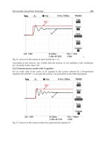
Example 1. Consider a two-link planar manipulator example (Fig. 1). First, only joint link
masses are considered for simplicity, as the one in [3, 6]. However, we take the correct
model in Corollary 1 and Remark 2 into account. The system parameters are: link mass
kgm 2
1
, kgm 10
2
, lengths ml 1
1
, ml 1
2
, angular positions q
1
, q
2
(rad), applied
torques f
1
, f
2
(Nm). Thus, the nominal values of coefficient matrices for the dynamic
equation (1) in Corollary 1 are:
)(
0
qM
10)1(10
)1(102022
2
22
C
CC
,
01
12
10),(
220
qSqqV
gqqN ),(
0
12
121
10
1012
C
CC
(39)
where
ii
qC cos , 2,1
i , )cos(
2112
qqC ,
22
sin qS , and g is the gravity accelera-
tion.
The desired trajectory is
)(tq
d
in (25) with 0
v
K , and
IK
p
, the signal
15.0)(tr , the initial values of the desired states
22)0(
d
q ,
0)0(
d
q
, i.e.,
5.0cos5.1)(
1
ttq
d
, and 1cos)(
2
ttq
d
(40)
The initial states are set as
2)0()0(
21
qq , and 0)0()0(
21
, i.e., 4)0(
1
e ,
4)0(
2
e , 0)0(
1
e
, and 0)0(
2
e
. The state variable is
][
eex
where qqe
d
.
The parametric uncertainties are assumed to satisfy (22) with 5.0
f
, 40
e
, 10
N
.
Select the adjustable parameters 012.0
1
, 0015.0
2
from (31), disturbance rejection
index
1.0
, the relative stability index 1.0
1
, and the left bound of vertical strip
2000
2
since we want a fast response. By Theorem 4, we solve the Riccati equation (32)
to get the solution matrix P and the gain matrix as:
22
22
16431584
158412693
II
II
P , ]7863.9851823.950[
22
IIPBrK
with 6.0r . The eigenvalues of the closed-loop main system matrix
BK
A are
{-0.9648, -0.9648, -984.8215, -984.8215}. Remark 5 gives the result
1873
2
. The
uncertain closed-loop system has its
12
)](Re[
c
A robustly.
The total control input (law) is
uMNqqqVqMFF
dTc 0000
),(
12
121
2
1
22
2
22
10
1012
01
12
10
cos
cos5.1
10)1(10
)1(102022
C
CC
g
q
q
qS
t
t
C
CC
e
e
II
C
CC
22
2
22
7863.9851823.950
10)1(10
)1(102022
(41)
A simulation for this example is taken with )(4.0)(
0
qMqM , i.e., 40% disturbance,
5.02857.0)()(
1
f
qMqM
, ),( qqV
m
),(2.0
0
qqV
m
with 20% disturbance, and
)(2.0)(
0
qNqN with 20% disturbance. The simulation results by MATLAB and Simulink
are shown in Figs. 2-3.
Fig. 2. States and their desired states: (a) )(
1
tq & )(
1
tq
d
, (b) )(
2
tq & )(
2
tq
d
in Example 1
ROBUSTCONTROLDESIGNFORTWO-LINKNONLINEARROBOTICSYSTEM 559
4. Examples
Example 1. Consider a two-link planar manipulator example (Fig. 1). First, only joint link
masses are considered for simplicity, as the one in [3, 6]. However, we take the correct
model in Corollary 1 and Remark 2 into account. The system parameters are: link mass
kgm 2
1
, kgm 10
2
, lengths ml 1
1
, ml 1
2
, angular positions q
1
, q
2
(rad), applied
torques f
1
, f
2
(Nm). Thus, the nominal values of coefficient matrices for the dynamic
equation (1) in Corollary 1 are:
)(
0
qM
10)1(10
)1(102022
2
22
C
CC
,
01
12
10),(
220
qSqqV
gqqN ),(
0
12
121
10
1012
C
CC
(39)
where
ii
qC cos , 2,1
i , )cos(
2112
qqC ,
22
sin qS , and g is the gravity accelera-
tion.
The desired trajectory is
)(tq
d
in (25) with 0
v
K , and
IK
p
, the signal
15.0)(tr , the initial values of the desired states
22)0(
d
q ,
0)0(
d
q
, i.e.,
5.0cos5.1)(
1
ttq
d
, and 1cos)(
2
ttq
d
(40)
The initial states are set as
2)0()0(
21
qq , and 0)0()0(
21
, i.e., 4)0(
1
e ,
4)0(
2
e , 0)0(
1
e
, and 0)0(
2
e
. The state variable is
][
eex
where qqe
d
.
The parametric uncertainties are assumed to satisfy (22) with 5.0
f
, 40
e
, 10
N
.
Select the adjustable parameters 012.0
1
, 0015.0
2
from (31), disturbance rejection
index
1.0
, the relative stability index 1.0
1
, and the left bound of vertical strip
2000
2
since we want a fast response. By Theorem 4, we solve the Riccati equation (32)
to get the solution matrix P and the gain matrix as:
22
22
16431584
158412693
II
II
P , ]7863.9851823.950[
22
IIPBrK
with 6.0r . The eigenvalues of the closed-loop main system matrix
BK
A are
{-0.9648, -0.9648, -984.8215, -984.8215}. Remark 5 gives the result
1873
2
. The
uncertain closed-loop system has its
12
)](Re[
c
A robustly.
The total control input (law) is
uMNqqqVqMFF
dTc 0000
),(
12
121
2
1
22
2
22
10
1012
01
12
10
cos
cos5.1
10)1(10
)1(102022
C
CC
g
q
q
qS
t
t
C
CC
e
e
II
C
CC
22
2
22
7863.9851823.950
10)1(10
)1(102022
(41)
A simulation for this example is taken with )(4.0)(
0
qMqM , i.e., 40% disturbance,
5.02857.0)()(
1
f
qMqM
, ),( qqV
m
),(2.0
0
qqV
m
with 20% disturbance, and
)(2.0)(
0
qNqN with 20% disturbance. The simulation results by MATLAB and Simulink
are shown in Figs. 2-3.
Fig. 2. States and their desired states: (a) )(
1
tq & )(
1
tq
d
, (b) )(
2
tq & )(
2
tq
d
in Example 1
AdvancesinRobotManipulators560
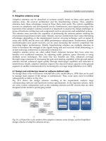
Fig. 3. Error signals: (a) e
1
(t), (b) e
2
(t) in Example 1
Example 2. Consider a two-link planar robotic system example with the joint mass and the
arm mass along the arm length. The mass of joint 1 is 1
1
m kg, and the mass of joint 2 is
5.0
2
m kg. The dimensions of two robot arms are linearly reduced round rods. The two
terminal radii of the arm rod 1 are
3
01
r cm and 2
1
t
r cm. The two terminal radii of the
arm rod 2 are
2
02
r cm and 1
1
t
r cm. Their end cross-sectional areas are
9
01
S cm
2
,
4
1
t
S cm
2
,
4
02
S cm
2
, and
1
2
t
S cm
2
. The arm length and mass are 1
1
l m,
1
2
l m, 2.5
1
r
m kg, and 9.1
2
r
m kg. By Theorem 3, it leads to:
2684.0
1
, 2286.0
2
, 4342.0
1
, 3929.0
2
(42)
By Theorem 3, the nominal model parameters are:
)(
0
qM
9343.02464.19343.0
2464.19343.04929.27301.5
2
22
C
CC
),(
0
qqV
01
12
2464.1
22
qS
),(
0
qqN
12
121
2464.1
2464.16579.5
C
CC
g (43)
The desired trajectory
)(tq
d
is the same as in Example 1. The initial states are set as
2)0(
1
q , 0)0(
2
q ,
)0(
1
q
0)0(
2
q
, i.e., 4)0(
1
e , 2)0(
2
e , 0)0(
1
e
, 0)0(
2
e
.
The parametric uncertainties in practice are assumed to satisfy (22) with
25.0
f
,
10
e
, 10
N
. Select the adjustable parameters 0375.0
1
and 0188.0
2
from
(31), the disturbance rejection index
1.0
, the relative stability index 1.0
1
, and the
left bound of vertical strip
100
2
. By Theorem 4, the solution matrix P to (32) and the
gain matrix K are
22
22
47.1255.13
55.1387.898
II
II
P ,
P
B
r
K
]8659.590589.65[
22
II
with
8.4r . The eigenvalues of the closed-loop main system matrix
BK
A are
{
1072.1 , 7587.58 , 1072.1
, 7587.58
}. The uncertain system has
12
)](Re[
c
A robustly.
The total control input (law) is :
uMNqqqVqMf
d 0000
),(
9343.02464.19343.0
2464.19343.04929.27301.5
2
22
C
CC
t
t
cos
cos5.1
01
12
2464.1
22
qS
2
1
q
q
12
121
2464.1
2464.16579.5
C
CC
g
+
9343.02464.19343.0
2464.19343.04929.27301.5
2
22
C
CC
22
8659.590589.65 II
ee
(44)
The simulation is taken with
)(25.0)(
0
qMqM
,
),(1.0),(
0
qqVqqV
mm
, and
)(1.0)(
0
qNqN . The results are shown in Figs. 4-5. It is noticed that the error may be
reduced when the gain parameter r is set large.
ROBUSTCONTROLDESIGNFORTWO-LINKNONLINEARROBOTICSYSTEM 561
Fig. 3. Error signals: (a) e
1
(t), (b) e
2
(t) in Example 1
Example 2. Consider a two-link planar robotic system example with the joint mass and the
arm mass along the arm length. The mass of joint 1 is 1
1
m kg, and the mass of joint 2 is
5.0
2
m kg. The dimensions of two robot arms are linearly reduced round rods. The two
terminal radii of the arm rod 1 are
3
01
r cm and 2
1
t
r cm. The two terminal radii of the
arm rod 2 are
2
02
r cm and 1
1
t
r cm. Their end cross-sectional areas are
9
01
S cm
2
,
4
1
t
S cm
2
,
4
02
S cm
2
, and
1
2
t
S cm
2
. The arm length and mass are 1
1
l m,
1
2
l m, 2.5
1
r
m kg, and 9.1
2
r
m kg. By Theorem 3, it leads to:
2684.0
1
, 2286.0
2
, 4342.0
1
, 3929.0
2
(42)
By Theorem 3, the nominal model parameters are:
)(
0
qM
9343.02464.19343.0
2464.19343.04929.27301.5
2
22
C
CC
),(
0
qqV
01
12
2464.1
22
qS
),(
0
qqN
12
121
2464.1
2464.16579.5
C
CC
g (43)
The desired trajectory
)(tq
d
is the same as in Example 1. The initial states are set as
2)0(
1
q , 0)0(
2
q ,
)0(
1
q
0)0(
2
q
, i.e., 4)0(
1
e , 2)0(
2
e , 0)0(
1
e
, 0)0(
2
e
.
The parametric uncertainties in practice are assumed to satisfy (22) with
25.0
f
,
10
e
, 10
N
. Select the adjustable parameters 0375.0
1
and 0188.0
2
from
(31), the disturbance rejection index
1.0
, the relative stability index 1.0
1
, and the
left bound of vertical strip
100
2
. By Theorem 4, the solution matrix P to (32) and the
gain matrix K are
22
22
47.1255.13
55.1387.898
II
II
P ,
P
B
r
K
]8659.590589.65[
22
II
with
8.4r . The eigenvalues of the closed-loop main system matrix
BK
A are
{
1072.1 , 7587.58 , 1072.1
, 7587.58
}. The uncertain system has
12
)](Re[
c
A robustly.
The total control input (law) is :
uMNqqqVqMf
d 0000
),(
9343.02464.19343.0
2464.19343.04929.27301.5
2
22
C
CC
t
t
cos
cos5.1
01
12
2464.1
22
qS
2
1
q
q
12
121
2464.1
2464.16579.5
C
CC
g
+
9343.02464.19343.0
2464.19343.04929.27301.5
2
22
C
CC
22
8659.590589.65 II
ee
(44)
The simulation is taken with
)(25.0)(
0
qMqM
,
),(1.0),(
0
qqVqqV
mm
, and
)(1.0)(
0
qNqN . The results are shown in Figs. 4-5. It is noticed that the error may be
reduced when the gain parameter r is set large.
AdvancesinRobotManipulators562
Fig. 4. States and their desired states: (a)
)(
1
tq & )(
1
tq
d
, (b) )(
2
tq & )(
2
tq
d
Fig. 5. Error signals: (a) e
1
(t), & (b) e
2
(t)
5. Conclusion
The chapter develops the practical models of two-link planar nonlinear robotic systems with
their arm distributed mass in addition to the joint-end mass. The new scaling coefficients
are introduced for solving this problem with the distributed mass along the arms. In
addition, Theorems 2 and 3 respectively present two special cases: a uniform arm shape (i.e.,
uniform distributed mass) and a linear reduction of arm shape along the arm length.
Based on the presented new models, an approach to design a continuous nonlinear control
law with a linear state-feedback control for the two-link planar robotic uncertain nonlinear
systems is presented in Theorem 4. The designed closed-loop systems possess the
properties of robust pole-clustering within a vertical strip on the left half s-plane and
disturbance rejection with an
H -norm constraint. The suggested robust control for the
uncertain nonlinear robotic systems can guarantee the required robust stability and
performance in face of parameter errors, state-dependent perturbations, unknown
parameters, frictions, load variation and disturbances for all allowed uncertainties in (22).
The presented robust control does always exist as pointed out in Remark 4. The adjustable
scalars
i
, i=1, 2, provide some flexibility in finding a solution of the algebraic Riccati
equation. The designed uncertain system has
1
-degree robust stabilization and
-degree
disturbance rejection. The controller gain parameter r is selected such that the designed
uncertain linear system achieves robust pole-clustering within a vertical strip. The examples
illustrate excellent results. This design procedure may be used for designing other control
systems, modeling, and simulation.
6. References
[1]J.J.Craig, Adaptive control of mechanical manipulators, Addison-Wesley (Publishing
Company, Inc., New York, 1988).
[2]J.H. Kaloust, & Z. Qu, Robust guaranteed cost control of uncertain nonlinear robotic sys-
tem using mixed minimum time and quadratic performance index, Proc. 32nd IEEE
Conf. on Decision and Control, 1993, 1634-1635.
[3]J. Kaneko, A robust motion control of manipulators with parametric uncertainties and
random disturbances, Proc. 34rd IEEE Conf. on Decision and Control, 1995, 1609-1610.
[4]R.L. Tummala, Dynamics and Control – Robotics, in The Electrical Engineering Handbook,
Ed. by R.C. Dorf, (2nd ed., CRC Press with IEEE Press, Boca Raton, FL, 1997, 2347).
[5]M. Garcia-Sanz, L. Egana, & J. Villanueva, “Interval Modelling of a SCARA Robot for
Robust Control”, Proc. 10
th
Mediterranean Conf. on Control and Automation, 2002.
[6]S. Lin, & S G. Wang, Robust Control with Pole Clustering for Uncertain Robotic Systems,
International Journal of Control and Intelligent Systems, 28(2), 2000, 72-79.
[7]S.B. Lin, and O. Masory, Gains selection of a variable gain adaptive control system for
turning, ASME Journal of Engineering for Industry, 109, 1987, 399-403.
[8]S G. Wang, L.S. Shieh, & J.W. Sunkel, Robust optimal pole-clustering in a vertical strip
and disturbance rejection for Lagrange’s systems, Int. J. Dynamics and Control, 5(3),
1995, 295-312.
ROBUSTCONTROLDESIGNFORTWO-LINKNONLINEARROBOTICSYSTEM 563
Fig. 4. States and their desired states: (a)
)(
1
tq & )(
1
tq
d
, (b) )(
2
tq & )(
2
tq
d
Fig. 5. Error signals: (a) e
1
(t), & (b) e
2
(t)
5. Conclusion
The chapter develops the practical models of two-link planar nonlinear robotic systems with
their arm distributed mass in addition to the joint-end mass. The new scaling coefficients
are introduced for solving this problem with the distributed mass along the arms. In
addition, Theorems 2 and 3 respectively present two special cases: a uniform arm shape (i.e.,
uniform distributed mass) and a linear reduction of arm shape along the arm length.
Based on the presented new models, an approach to design a continuous nonlinear control
law with a linear state-feedback control for the two-link planar robotic uncertain nonlinear
systems is presented in Theorem 4. The designed closed-loop systems possess the
properties of robust pole-clustering within a vertical strip on the left half s-plane and
disturbance rejection with an
H -norm constraint. The suggested robust control for the
uncertain nonlinear robotic systems can guarantee the required robust stability and
performance in face of parameter errors, state-dependent perturbations, unknown
parameters, frictions, load variation and disturbances for all allowed uncertainties in (22).
The presented robust control does always exist as pointed out in Remark 4. The adjustable
scalars
i
, i=1, 2, provide some flexibility in finding a solution of the algebraic Riccati
equation. The designed uncertain system has
1
-degree robust stabilization and
-degree
disturbance rejection. The controller gain parameter r is selected such that the designed
uncertain linear system achieves robust pole-clustering within a vertical strip. The examples
illustrate excellent results. This design procedure may be used for designing other control
systems, modeling, and simulation.
6. References
[1]J.J.Craig, Adaptive control of mechanical manipulators, Addison-Wesley (Publishing
Company, Inc., New York, 1988).
[2]J.H. Kaloust, & Z. Qu, Robust guaranteed cost control of uncertain nonlinear robotic sys-
tem using mixed minimum time and quadratic performance index, Proc. 32nd IEEE
Conf. on Decision and Control, 1993, 1634-1635.
[3]J. Kaneko, A robust motion control of manipulators with parametric uncertainties and
random disturbances, Proc. 34rd IEEE Conf. on Decision and Control, 1995, 1609-1610.
[4]R.L. Tummala, Dynamics and Control – Robotics, in The Electrical Engineering Handbook,
Ed. by R.C. Dorf, (2nd ed., CRC Press with IEEE Press, Boca Raton, FL, 1997, 2347).
[5]M. Garcia-Sanz, L. Egana, & J. Villanueva, “Interval Modelling of a SCARA Robot for
Robust Control”, Proc. 10
th
Mediterranean Conf. on Control and Automation, 2002.
[6]S. Lin, & S G. Wang, Robust Control with Pole Clustering for Uncertain Robotic Systems,
International Journal of Control and Intelligent Systems, 28(2), 2000, 72-79.
[7]S.B. Lin, and O. Masory, Gains selection of a variable gain adaptive control system for
turning, ASME Journal of Engineering for Industry, 109, 1987, 399-403.
[8]S G. Wang, L.S. Shieh, & J.W. Sunkel, Robust optimal pole-clustering in a vertical strip
and disturbance rejection for Lagrange’s systems, Int. J. Dynamics and Control, 5(3),
1995, 295-312.
AdvancesinRobotManipulators564
[9]S G. Wang, L.S. Shieh, & J.W. Sunkel, Robust optimal pole-placement in a vertical strip
and disturbance rejection, Proc. 32nd IEEE Conf. on Decision and Control, 1993, 1134-
1139. Int. J. Systems Science, 26(10), 1995, 1839-1853.
[10]S G. Wang, S.B. Lin, L.S. Shieh, & J.W. Sunkel, Observer-based controller for robust pole
clustering in a vertical strip and disturbance rejection in structured uncertain
systems, Int. J. Robust & Nonlinear Control, 8(3), 1998, 1073-1084.
[11]J.J. Craig, Introduction to Robotics: Mechanics and Control (2nd ed., Addison-Weeley
Publishing Company, Inc., New York, 1988).
RoleofFiniteElementAnalysisinDesigningMulti-axesPositioningforRoboticManipulators 565
RoleofFiniteElementAnalysisinDesigningMulti-axesPositioningfor
RoboticManipulators
T.T.Mon,F.R.MohdRomlayandM.N.Tamin
x
Role of Finite Element Analysis in
Designing Multi-axes Positioning
for Robotic Manipulators
T.T. Mon, F.R. Mohd Romlay and M.N. Tamin
Universiti Malaysia Pahang, Universiti Teknology Malaysia
Malaysia
1. Introduction
Simulation of robot manipulator in Matlab/Simulink or any other mechanism simulator is
very common for robot design. However, all these approaches are mainly concerned with
design configuration having little analysis meaning that the robot model is formed by
linking the kinematics and solid description, and simulated for alternative configuration of
movements (Cleery & Mathur, 2008). Indeed comprehensive design should have analysis at
different computational levels. Finite element method (FEM) has been a major tool to
develop a computational model in various fields of studies because of its modelling and
simulation capability close to reality. Subsequently, modelling and analysis with FEM has
become the most convenient way to economically design and analyze real world problems,
either in static or dynamic. As a result, huge amount of reports on this topic can be found in
the literature (Mackerle, 1999). Unfortunately however, this technique has not
comprehensively applied in designing in designing a robot while choosing the best
components for the design is as important as having good performance and no
environmental impact of the machines over its lifetime. Building block of a robot
manipulator is electromechanical system in which mechanical systems are controlled by
sophisticated electric motor drives. Since energy saving everywhere is a major challenge
now and in future, getting electromechanical design right will significantly contribute to
energy saving.
This chapter is dedicated to the application of Finite Element Method (FEM) in designing
multi-axes positioning for robot manipulators. Computational model that can predict
physical behaviour of dynamic robot manipulators constructed using FE codes is presented,
and this is major contribution of the chapter. FEM tools necessary for modelling and
analysis of multi-axes positioning are presented in large part. Rather than a FEM discourse,
FEM is presented by highlighting mathematics behind and an application example as they
relates to practical robotic manipulation. It is, however, assumed that the reader has
acquired some basic knowledge of FEM consistent with the expected level of mathematics.
Hence, the chapter is organized as follows.
In the early part of the chapter, the important terminologies used in robotics are defined in
the background. The material is presented using a number of examples as evidenced in the
28
AdvancesinRobotManipulators566
published reports. Then the chapter will go to mathematics behind finite element modelling
and analysis of kinematics of a structure in 3D space as robotics involves tracking moving
objects in 3D space. This will also include mathematical tools essential for the study of
robotics, particularly matrix transforms, mathematical models of robot manipulators, direct
kinematic equations, inverse kinematic technique and Jacobian matrix needed to control
position and motion of a robot manipulator. More emphasis will be on how these
mathematical tools can be linked to and incorporated into FEM to carry out design analysis
of robot structure.
The rest of the chapter will present application of FEM in practical robot design, detailed
development of FE model computable for multi-axes positioning using a particular FE code
(ALGOR, 2008), and useful results predicted by the computational model. The chapter will
be closed by concluding remarks to choice of FE codes and its impact on the computational
model and finally the usefulness of computational model.
2. Background in Robotics
Multi-axis positioning meant here is different movements of a point, or a structure in
different directions. This term is drawn from the term usually come with computer
numerical controlled machines just as 3-axis, 5-axis and so on, where the 3-axis machine, for
instance, implies that it can make a maximum of three different positioning of the controlled
elements. Each axis is alternatively referred to as degree of freedom (DOF) that is something
to do with motion in a system or a structure. Since the term ‘axis’ is adopted to represent an
element that creates motion, 3-axis positioning means three DOF’s, for example (Rahman,
2004). In relation to these definitions, one manipulator of a robot can represent one axis or
DOF as the manipulator is the robot’s arm, a movable mechanical unit comprising of
segments or links jointed together with axes capable of motion in various directions
allowing the robot to perform tasks. Typically, the body, arm and wrist are components of
manipulators. Movements between the various components of the manipulator are
provided by series of joints.
The points that a manipulator bends, slides or rotates are called joints or position axes.
Position axes are also called the world coordinates. The world coordinate system is usually
identified as being a fixed location within the manipulator that serves as an absolute frame
of reference.
In general, the manipulator’s motion can be divided into two categories: translation and
rotation. Although one can further categorize it in specific term such as a pitch (up-and-
down motion); a yaw (side-to-side motion); and a roll (rotating motion), any of these is fall
into either translation or rotation. The individual joint motion associated with either of these
two categories is referred to degree of freedom. Subsequently, one degree of freedom is
equal to one axis. The industrial robots are typically equipped with 4-6 axes.
The power supply provides the energy required for a robot to be operated. Electricity is the
most common source of power and is used extensively with industrial robots. Payload is the
weight that the robot is designed to lift, hold, and position repeatedly with the same
accuracy. Hence, the power supply has direct relation to the payload rating of a robot.
Among the important dynamic properties of a robot that properly regulates its motion are:
stability, control resolution, spatial resolution, accuracy, repeatability and compliance. To
take these factors into account in the design of a robot is a complex issue. Lack of stability
occurs very often due to wear of manipulator components, movement longer than the
intended, longer time to reach and overshooting of position.
Control resolution is all about position control. It is a function of the design of robot control
system and specifies the smallest increment of motion by which the system can divide its
working space. It is the smallest incremental change in position that its control system can
measure. In other words, it is the controller’s ability to divide the total range of movements
for the particular joint into individual increments that can be addressed in the controller.
This depends on the bit storage capacity in the control memory. For example, a robot with 8
bits of storage can divide the range into 256 discrete positions. The control resolution would
be also defined as the total motion range divided by the number of increments. For example,
a robot has one sliding joint with a full range of 1.0 m. The robot control memory has 12-bit
storage capacity. The control resolution for this axis of motion is 0.244mm. The spatial
resolution of a robot is the smallest increment of movement into which the robot can divide
its work volume.
Mechanical inaccuracies in the robot’s links and joint components and its feedback
measurements system (if it is a servo-controlled robot) constitute the other factor that
contributes to spatial resolution. Mechanical inaccuracies come from elastic deflection in the
structural members, gear backlash, stretching of pulley cords and other imperfections in the
mechanical system. These inaccuracies tend to be worse for large robot simply because the
errors are magnified by the large components. The spatial resolution is degraded by these
mechanical inaccuracies.
Rigidity of the structure also affects the repeatability of the robot. Compliance is a quality
that gives a manipulator of a robot the ability to tolerate misalignment of mating parts. It is
essential for assembly of close-fitting parts. In an electric manipulator, the motors generally
connect to mechanical coupling. The sticking and sliding friction in such a coupling can
cause a strange effect on the compliance, in particular, being back-drivable.
An Off-line programming system includes a spatial representation of solids and their
graphical interpretation, automatic collision detection, incorporation of kinematic, path
planning and dynamic simulation and concurrent programming. The off-line programming
will grow more in the future because of graphical computer simulation used to validate
program development. It is important both as aids in programming industrial automation
and as platforms for robotic research (Billingsley, 1985; Keramas, 1999; Angeles, 2003).
3. Mathematical Foundation
Forward and reverse kinematics methods are the principal mathematics behind typical
modeling, computation and analysis of robot manipulators. Since the latter is deduced from
the former, broader review will focus on some related mathematics of the former. Forward
kinematic equation relates a pose element to the joint variables. The pose matrix is
computed from the joint variables. The position and orientation of end-manipulator (also-
called the end-effector, the last joint that directly touches and handles the object) is
computed from all joint variables. The position and orientation of the end manipulator are
computed from a set of joint variable values which are already known or specified. The
computation follows the arrow directions starting from joint 1 as illustrated in Fig. 1. It
should be noted that in kinematics analysis, the manipulators are assumed to be rigid.
RoleofFiniteElementAnalysisinDesigningMulti-axesPositioningforRoboticManipulators 567
published reports. Then the chapter will go to mathematics behind finite element modelling
and analysis of kinematics of a structure in 3D space as robotics involves tracking moving
objects in 3D space. This will also include mathematical tools essential for the study of
robotics, particularly matrix transforms, mathematical models of robot manipulators, direct
kinematic equations, inverse kinematic technique and Jacobian matrix needed to control
position and motion of a robot manipulator. More emphasis will be on how these
mathematical tools can be linked to and incorporated into FEM to carry out design analysis
of robot structure.
The rest of the chapter will present application of FEM in practical robot design, detailed
development of FE model computable for multi-axes positioning using a particular FE code
(ALGOR, 2008), and useful results predicted by the computational model. The chapter will
be closed by concluding remarks to choice of FE codes and its impact on the computational
model and finally the usefulness of computational model.
2. Background in Robotics
Multi-axis positioning meant here is different movements of a point, or a structure in
different directions. This term is drawn from the term usually come with computer
numerical controlled machines just as 3-axis, 5-axis and so on, where the 3-axis machine, for
instance, implies that it can make a maximum of three different positioning of the controlled
elements. Each axis is alternatively referred to as degree of freedom (DOF) that is something
to do with motion in a system or a structure. Since the term ‘axis’ is adopted to represent an
element that creates motion, 3-axis positioning means three DOF’s, for example (Rahman,
2004). In relation to these definitions, one manipulator of a robot can represent one axis or
DOF as the manipulator is the robot’s arm, a movable mechanical unit comprising of
segments or links jointed together with axes capable of motion in various directions
allowing the robot to perform tasks. Typically, the body, arm and wrist are components of
manipulators. Movements between the various components of the manipulator are
provided by series of joints.
The points that a manipulator bends, slides or rotates are called joints or position axes.
Position axes are also called the world coordinates. The world coordinate system is usually
identified as being a fixed location within the manipulator that serves as an absolute frame
of reference.
In general, the manipulator’s motion can be divided into two categories: translation and
rotation. Although one can further categorize it in specific term such as a pitch (up-and-
down motion); a yaw (side-to-side motion); and a roll (rotating motion), any of these is fall
into either translation or rotation. The individual joint motion associated with either of these
two categories is referred to degree of freedom. Subsequently, one degree of freedom is
equal to one axis. The industrial robots are typically equipped with 4-6 axes.
The power supply provides the energy required for a robot to be operated. Electricity is the
most common source of power and is used extensively with industrial robots. Payload is the
weight that the robot is designed to lift, hold, and position repeatedly with the same
accuracy. Hence, the power supply has direct relation to the payload rating of a robot.
Among the important dynamic properties of a robot that properly regulates its motion are:
stability, control resolution, spatial resolution, accuracy, repeatability and compliance. To
take these factors into account in the design of a robot is a complex issue. Lack of stability
occurs very often due to wear of manipulator components, movement longer than the
intended, longer time to reach and overshooting of position.
Control resolution is all about position control. It is a function of the design of robot control
system and specifies the smallest increment of motion by which the system can divide its
working space. It is the smallest incremental change in position that its control system can
measure. In other words, it is the controller’s ability to divide the total range of movements
for the particular joint into individual increments that can be addressed in the controller.
This depends on the bit storage capacity in the control memory. For example, a robot with 8
bits of storage can divide the range into 256 discrete positions. The control resolution would
be also defined as the total motion range divided by the number of increments. For example,
a robot has one sliding joint with a full range of 1.0 m. The robot control memory has 12-bit
storage capacity. The control resolution for this axis of motion is 0.244mm. The spatial
resolution of a robot is the smallest increment of movement into which the robot can divide
its work volume.
Mechanical inaccuracies in the robot’s links and joint components and its feedback
measurements system (if it is a servo-controlled robot) constitute the other factor that
contributes to spatial resolution. Mechanical inaccuracies come from elastic deflection in the
structural members, gear backlash, stretching of pulley cords and other imperfections in the
mechanical system. These inaccuracies tend to be worse for large robot simply because the
errors are magnified by the large components. The spatial resolution is degraded by these
mechanical inaccuracies.
Rigidity of the structure also affects the repeatability of the robot. Compliance is a quality
that gives a manipulator of a robot the ability to tolerate misalignment of mating parts. It is
essential for assembly of close-fitting parts. In an electric manipulator, the motors generally
connect to mechanical coupling. The sticking and sliding friction in such a coupling can
cause a strange effect on the compliance, in particular, being back-drivable.
An Off-line programming system includes a spatial representation of solids and their
graphical interpretation, automatic collision detection, incorporation of kinematic, path
planning and dynamic simulation and concurrent programming. The off-line programming
will grow more in the future because of graphical computer simulation used to validate
program development. It is important both as aids in programming industrial automation
and as platforms for robotic research (Billingsley, 1985; Keramas, 1999; Angeles, 2003).
3. Mathematical Foundation
Forward and reverse kinematics methods are the principal mathematics behind typical
modeling, computation and analysis of robot manipulators. Since the latter is deduced from
the former, broader review will focus on some related mathematics of the former. Forward
kinematic equation relates a pose element to the joint variables. The pose matrix is
computed from the joint variables. The position and orientation of end-manipulator (also-
called the end-effector, the last joint that directly touches and handles the object) is
computed from all joint variables. The position and orientation of the end manipulator are
computed from a set of joint variable values which are already known or specified. The
computation follows the arrow directions starting from joint 1 as illustrated in Fig. 1. It
should be noted that in kinematics analysis, the manipulators are assumed to be rigid.
AdvancesinRobotManipulators568
3.1 Defining the location of an object in space
As a general case, the object location in 3D space is considered. A matrix representation is
widely used to represent the object location as it is convenient and easy to handle especially
when the location is changed. Two parameters are needed to define the object location:
position and orientation. Basically, a homogenous vector ‘v’ is represented as
(1)
if v is a free vector or
(2)
if v represents the position of a particular point in the usual coordinates system (x, y, and z).
This coordinates system is referred to a frame. These frames are used to track an object
location in space. As shown in Fig. 2, the frame F
o
is attached to a fixed point while another
F
A
to an object. The object position is described by the vector pA of the origin A of the frame
F
A
. The orientation of the object is given by the homogeneous vectors of each unit vectors
x
A
, y
A
and z
A
of F
A
with respect to F
o
.
Then the object location is mathematically represented by a post matrix ‘P’ as:
(3)
where the matrix
(4)
and
(5)
formed by the coordinates of the vectors xA, yA and zA is a rotation matrix that holds the
orientation of the object while the p
A
holds the position of the object. In a compact form, the
pose matrix can be written as:
(6)
where O refers to a 1x3 vector of zeros.
Fig. 1. Forward kinematics
Fig. 2. The object with respect to frames.
When a point, say Q given by its coordinate vector
A
q = with respect to frame F
A
, is
transformed to the frame F
O
, the transformed vector say
o
q can be expressed as:
RoleofFiniteElementAnalysisinDesigningMulti-axesPositioningforRoboticManipulators 569
3.1 Defining the location of an object in space
As a general case, the object location in 3D space is considered. A matrix representation is
widely used to represent the object location as it is convenient and easy to handle especially
when the location is changed. Two parameters are needed to define the object location:
position and orientation. Basically, a homogenous vector ‘v’ is represented as
(1)
if v is a free vector or
(2)
if v represents the position of a particular point in the usual coordinates system (x, y, and z).
This coordinates system is referred to a frame. These frames are used to track an object
location in space. As shown in Fig. 2, the frame F
o
is attached to a fixed point while another
F
A
to an object. The object position is described by the vector pA of the origin A of the frame
F
A
. The orientation of the object is given by the homogeneous vectors of each unit vectors
x
A
, y
A
and z
A
of F
A
with respect to F
o
.
Then the object location is mathematically represented by a post matrix ‘P’ as:
(3)
where the matrix
(4)
and
(5)
formed by the coordinates of the vectors xA, yA and zA is a rotation matrix that holds the
orientation of the object while the p
A
holds the position of the object. In a compact form, the
pose matrix can be written as:
(6)
where O refers to a 1x3 vector of zeros.
Fig. 1. Forward kinematics
Fig. 2. The object with respect to frames.
When a point, say Q given by its coordinate vector
A
q = with respect to frame F
A
, is
transformed to the frame F
O
, the transformed vector say
o
q can be expressed as:
AdvancesinRobotManipulators570
(7)
In compact form
o
q =
o
T
A
A
q
(8)
where
o
T
A
= P
Similarly in alternative representation of frame transforms, simple space translation and
rotation can be conveniently represented as a compact-form matrix as:
T
q = T
u
q
R
q = R
v,θ
q
(9)
(10)
where q = is coordinates vector of a point Q, T
u
is a translation vector, R
v,θ
is a rotation
vector,
T
q is coordinates vector of a point Q' where Q is translated by T
u
and
R
q coordinates
vector of a point Q' where Q is rotated around v by an angle θ.
Furthermore, the translations and rotations along the reference axes, called canonical
translations/rotations, have the homogeneous matrix of the following form respectively as:
(11)
(12)
(13)
(14)
(15)
(16)
Where
are translations of a distance, ‘d’ in x, y and z directions
respectively, and are rotations about the respective axis by
the respective angle with and These can be expanded to
arbitrary transformations. Refer to Manseur (2006) for details.
3.2 DH parameters
In the conventional analysis of motion of robot manipulators, the Denavit-Hartenberg (DH)
modelling technique is commonly used as a standard technique. Reference frames are
assigned to each link based on DH parameters, starting from the fixed link all the way to the
last link. The DH model is obtained by describing each link frame with respect to the
preceding link frame. The original representation of one frame with respect to another using
pose matrix requires a minimum of six parameters. The DH modelling technique reduces
these parameters to four, routinely noted as:
di, the link offset,
ai, the link length,
θi, the link angle and
αi, the link twist as illustrated in Fig. 3.
di
Zi-1
Xi-1
Fi-1
Fi
Xi
Zi
αi
θi
ai
Fig. 3. Illustration of DH parameters
RoleofFiniteElementAnalysisinDesigningMulti-axesPositioningforRoboticManipulators 571
(7)
In compact form
o
q =
o
T
A
A
q
(8)
where
o
T
A
= P
Similarly in alternative representation of frame transforms, simple space translation and
rotation can be conveniently represented as a compact-form matrix as:
T
q = T
u
q
R
q = R
v,θ
q
(9)
(10)
where q = is coordinates vector of a point Q, T
u
is a translation vector, R
v,θ
is a rotation
vector,
T
q is coordinates vector of a point Q' where Q is translated by T
u
and
R
q coordinates
vector of a point Q' where Q is rotated around v by an angle θ.
Furthermore, the translations and rotations along the reference axes, called canonical
translations/rotations, have the homogeneous matrix of the following form respectively as:
(11)
(12)
(13)
(14)
(15)
(16)
Where
are translations of a distance, ‘d’ in x, y and z directions
respectively, and
are rotations about the respective axis by
the respective angle with
and These can be expanded to
arbitrary transformations. Refer to Manseur (2006) for details.
3.2 DH parameters
In the conventional analysis of motion of robot manipulators, the Denavit-Hartenberg (DH)
modelling technique is commonly used as a standard technique. Reference frames are
assigned to each link based on DH parameters, starting from the fixed link all the way to the
last link. The DH model is obtained by describing each link frame with respect to the
preceding link frame. The original representation of one frame with respect to another using
pose matrix requires a minimum of six parameters. The DH modelling technique reduces
these parameters to four, routinely noted as:
di, the link offset,
ai, the link length,
θi, the link angle and
αi, the link twist as illustrated in Fig. 3.
di
Zi-1
Xi-1
Fi-1
Fi
Xi
Zi
αi
θi
a
i
Fig. 3. Illustration of DH parameters
AdvancesinRobotManipulators572
Referring to Fig. 4, in relation to the link frames and DH parameters, homogenous frame
transform from the frame (i) to (i-1) can be generally written as
i-1
A
i
=
(17)
where T(z, di ) is translation from Fi-1 to Fd, R(z, θi ) the rotation transform from Fd to Fθ,
T(x, ai ) the translation transform from Fθ to Fa, R(x, αi) the rotation transform from Fa to
Fi.
Fig. 4. Frame transformation of the DH parameters.
The matrix
i-1
A
i
is then used to express the transform of the end frame to the base frame for
‘n-axis’ or ‘n-joint’ robot manipulators. That is
=
(18)
or
(19)
where
= pose matrix of the end-effector. This process is
called forward kinematic in modelling, computation and analysis of robotic manipulator.
In the reverse kinematics method, as it means, one or more sets of joint variables are
computed from the known end-effector pose matrix. As such the direction of computation is
revered from that of the forward kinematics as illustrated in Fig.5. Nevertheless, the same
basic concept of forward kinematics is applied except the fact that the mathematical
manipulation becomes different and sophisticated. To be brief, the equations derived from
the forward kinematics method are reduced to a set of equations involving as few unknown
joint variables as possible using a kinematic function that depends on only certain joint
variables. This results simplified set of equation that can be solved analytically. Details can
be found elsewhere (Manseur, 2006).
Fig. 5. Reverse kinematics
3.3 Velocity Kinematics
When the time factor is taken into account in the movement of a manipulator, Jacobian
matrix is used to manipulate the transformation of manipulator. The generalized velocity
vector V of the end-effector with respect to the base frame can be a form of a linear velocity
vector v and an angular velocity vector ω:
(20)
where
(21)
and
RoleofFiniteElementAnalysisinDesigningMulti-axesPositioningforRoboticManipulators 573
Referring to Fig. 4, in relation to the link frames and DH parameters, homogenous frame
transform from the frame (i) to (i-1) can be generally written as
i-1
A
i
=
(17)
where T(z, di ) is translation from Fi-1 to Fd, R(z, θi ) the rotation transform from Fd to Fθ,
T(x, ai ) the translation transform from Fθ to Fa, R(x, αi) the rotation transform from Fa to
Fi.
Fig. 4. Frame transformation of the DH parameters.
The matrix
i-1
A
i
is then used to express the transform of the end frame to the base frame for
‘n-axis’ or ‘n-joint’ robot manipulators. That is
=
(18)
or
(19)
where = pose matrix of the end-effector. This process is
called forward kinematic in modelling, computation and analysis of robotic manipulator.
In the reverse kinematics method, as it means, one or more sets of joint variables are
computed from the known end-effector pose matrix. As such the direction of computation is
revered from that of the forward kinematics as illustrated in Fig.5. Nevertheless, the same
basic concept of forward kinematics is applied except the fact that the mathematical
manipulation becomes different and sophisticated. To be brief, the equations derived from
the forward kinematics method are reduced to a set of equations involving as few unknown
joint variables as possible using a kinematic function that depends on only certain joint
variables. This results simplified set of equation that can be solved analytically. Details can
be found elsewhere (Manseur, 2006).
Fig. 5. Reverse kinematics
3.3 Velocity Kinematics
When the time factor is taken into account in the movement of a manipulator, Jacobian
matrix is used to manipulate the transformation of manipulator. The generalized velocity
vector V of the end-effector with respect to the base frame can be a form of a linear velocity
vector v and an angular velocity vector ω:
(20)
where
(21)
and
AdvancesinRobotManipulators574
(22)
For the case of n-joint robot, the relationship between the V and the joint velocities can
generally be expressed as
(23)
Where q =
is the joint variable and =
is corresponding velocity vector. The matrix J(q) is called the Jacobian matrix. It is the
mathematical relationship between joint motion and end-effector motion. It plays an
important role in the analysis and control of robotic motion owing to the fact that it
establishes a linear relation between velocity vectors in Cartesian space and in joint space.
Details of derivation of J and its computation can be found in (Manseur, 2006).
3.4 Typical Robot Simulators
Nowadays softwares are readily available to generate and solve the kinematic equations.
BUILD, SKEG and SIMULINK are some of those. Typical robot simulators allow the
programming of a manipulator positioning in Cartesian space and relate a Cartesian co-
ordinate set to the robot model’s joint angles known as the inverse kinematics
transformation (Zlajpah, 2008).
Kinematic description is made up of joint rotation and position information. The inverse
kinematic links the kinematics and solid descriptions. During the linking process, a
sequence of procedure is called to solve a particular position of the robot. For example, the
method of solving 6 DOFs robot as shown in Fig. 6 requires the following steps:
i. From tool position and orientation, calculate wrist position
ii. Calculate angle of rotation of axis 1
iii. Calculate angle 2 and 3 from the two link mechanism connecting the
shoulder and the wrist
iv. Calculate the remaining joint angles using spherical trigonometry [1]
Robot simulators do not allow dynamic effects or systematic errors in either trajectory
calculation or inverse kinematic processing. The implementation of a full dynamic model
would be out of question for a general simulator (e.g. BUILD simulator).
Robot errors can be categorized into two: static error related to end points and dynamic
error related to path. The formers result from deviation of the achieved position from the
demand position. The latter comes from mismatch between a desired path and the true path.
The computation of such information is very appropriate for a solid modelling system in
which methods for analyzing space are well developed. However in these simulations, there
will be differences between the actual robot performance and the modelled robot
performance. The difference will depend on the assumptions made when designing robot
model.
A particular robot’s physical kinematics will deviate from the idealized model due to
manufacturing tolerances and this will lead to a reduction in the accuracy of the robot’s
positioning with respect to a Cartesian space. The weight affects inaccuracies due to
compliance of robot manipulators (Billingsley, 1985).
Fig. 6. Robot with 6 DOFs.
To sum up, in conventional modelling technique, the robot manipulators are modelled as a
kinematic model. The accuracy of simulated motion in this technique is questionable.
Additionally, the model is inadequate for the analysis of the dynamics laws of motion in
which inertial parameters, link masses and shapes, and applied forces and torques must be
considered. This is where FEM comes into play.
4. Finite Element Method
It is hard to completely define finite element method (FEM) in one sentence or even a
paragraph. One may define it as a numerical method for solving engineering problem and
physics, or a method to computationally model reality in a mathematical form; either one is
acceptable indeed. However, for more complete definition of FEM, the following paragraph
may suit it better.
“A continuum is discretized into simple geometric shapes called finite elements; constitutive
relations, loading and constraints are defined over these elements; assembly of elements
results set of equations; solution of these equations gives the approximate behaviour of the
continuum.”
The procedure of using FEM to analyze the system behaviour generally includes:
RoleofFiniteElementAnalysisinDesigningMulti-axesPositioningforRoboticManipulators 575
(22)
For the case of n-joint robot, the relationship between the V and the joint velocities can
generally be expressed as
(23)
Where q = is the joint variable and =
is corresponding velocity vector. The matrix J(q) is called the Jacobian matrix. It is the
mathematical relationship between joint motion and end-effector motion. It plays an
important role in the analysis and control of robotic motion owing to the fact that it
establishes a linear relation between velocity vectors in Cartesian space and in joint space.
Details of derivation of J and its computation can be found in (Manseur, 2006).
3.4 Typical Robot Simulators
Nowadays softwares are readily available to generate and solve the kinematic equations.
BUILD, SKEG and SIMULINK are some of those. Typical robot simulators allow the
programming of a manipulator positioning in Cartesian space and relate a Cartesian co-
ordinate set to the robot model’s joint angles known as the inverse kinematics
transformation (Zlajpah, 2008).
Kinematic description is made up of joint rotation and position information. The inverse
kinematic links the kinematics and solid descriptions. During the linking process, a
sequence of procedure is called to solve a particular position of the robot. For example, the
method of solving 6 DOFs robot as shown in Fig. 6 requires the following steps:
i. From tool position and orientation, calculate wrist position
ii. Calculate angle of rotation of axis 1
iii. Calculate angle 2 and 3 from the two link mechanism connecting the
shoulder and the wrist
iv. Calculate the remaining joint angles using spherical trigonometry [1]
Robot simulators do not allow dynamic effects or systematic errors in either trajectory
calculation or inverse kinematic processing. The implementation of a full dynamic model
would be out of question for a general simulator (e.g. BUILD simulator).
Robot errors can be categorized into two: static error related to end points and dynamic
error related to path. The formers result from deviation of the achieved position from the
demand position. The latter comes from mismatch between a desired path and the true path.
The computation of such information is very appropriate for a solid modelling system in
which methods for analyzing space are well developed. However in these simulations, there
will be differences between the actual robot performance and the modelled robot
performance. The difference will depend on the assumptions made when designing robot
model.
A particular robot’s physical kinematics will deviate from the idealized model due to
manufacturing tolerances and this will lead to a reduction in the accuracy of the robot’s
positioning with respect to a Cartesian space. The weight affects inaccuracies due to
compliance of robot manipulators (Billingsley, 1985).
Fig. 6. Robot with 6 DOFs.
To sum up, in conventional modelling technique, the robot manipulators are modelled as a
kinematic model. The accuracy of simulated motion in this technique is questionable.
Additionally, the model is inadequate for the analysis of the dynamics laws of motion in
which inertial parameters, link masses and shapes, and applied forces and torques must be
considered. This is where FEM comes into play.
4. Finite Element Method
It is hard to completely define finite element method (FEM) in one sentence or even a
paragraph. One may define it as a numerical method for solving engineering problem and
physics, or a method to computationally model reality in a mathematical form; either one is
acceptable indeed. However, for more complete definition of FEM, the following paragraph
may suit it better.
“A continuum is discretized into simple geometric shapes called finite elements; constitutive
relations, loading and constraints are defined over these elements; assembly of elements
results set of equations; solution of these equations gives the approximate behaviour of the
continuum.”
The procedure of using FEM to analyze the system behaviour generally includes: