Advances in Robot Manipulators Part 13 pdf

Bạn đang xem bản rút gọn của tài liệu. Xem và tải ngay bản đầy đủ của tài liệu tại đây (5.55 MB, 40 trang )

AdvancesinRobotManipulators472

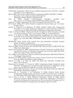
Although the actuating forces can be decreased by varying the orientations of the moving
platform, the required maximum leg lengths increase as indicated in Figs. 8(a), (b). It means
that a larger task space is necessary to accommodate the planned singularity-free path.
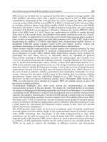
(2) Time optimum
For this problem, the travel time
f
t is to be determined. Based on the singularity-free path
planning algorithm, the planned trajectory is shown in Fig.9 (i.e. the line for
μ
=1) with the
corresponding minimal travel time
f
t =5.85 sec.

Fig. 6. Variations of determinant along corresponding planned paths

(a) (b)
Fig. 7. Actuating forces along planned paths with (a) constant orientation and (b) varied
orientations

(3) Energy efficiency
Fig. 9 also shows the minimal-energy trajectory with the corresponding travel time
f
t =20.01
sec (i.e. the line for
μ
=0). Compared with the time optimal trajectory planning, reduction in
the travel time is at the expense of a greater consumed energy, a poorer fitness value, and a
larger force.
(4) Mixed cost function

The cost function is defined as

1


t
T
f
t
G
μ
λ Δt
μ
dt
0
( ) + ( )= -
f
l (36)

The optimal singular free trajectories for
μ
=0.3, 0.6 and 0.8 with the corresponding
determined travel time
f
t =7.758, 6.083 and 6.075 sec are also respectively shown in Fig. 9.

(a)

(b)
Fig. 8. Leg lengths along planned paths with (a) constant orientation and (b) varied
orientations

5. Conclusions

In this chapter, a numerical technique is presented to determine the singularity-free

trajectories of a parallel robot manipulator. The required closed-form dynamic equations for
the parallel manipulator with a completely general architecture and inertia distribution are
OntheOptimalSingularity-FreeTrajectoryPlanningofParallelRobotManipulators 473

Although the actuating forces can be decreased by varying the orientations of the moving
platform, the required maximum leg lengths increase as indicated in Figs. 8(a), (b). It means
that a larger task space is necessary to accommodate the planned singularity-free path.
(2) Time optimum
For this problem, the travel time
f
t is to be determined. Based on the singularity-free path
planning algorithm, the planned trajectory is shown in Fig.9 (i.e. the line for
μ
=1) with the
corresponding minimal travel time
f
t =5.85 sec.

Fig. 6. Variations of determinant along corresponding planned paths

(a) (b)
Fig. 7. Actuating forces along planned paths with (a) constant orientation and (b) varied
orientations

(3) Energy efficiency
Fig. 9 also shows the minimal-energy trajectory with the corresponding travel time
f
t =20.01
sec (i.e. the line for
μ
=0). Compared with the time optimal trajectory planning, reduction in
the travel time is at the expense of a greater consumed energy, a poorer fitness value, and a
larger force.
(4) Mixed cost function

The cost function is defined as

1


t
T
f
t
G
μ
λ Δt
μ
dt
0
( ) + ( )= -
f
l (36)

The optimal singular free trajectories for
μ
=0.3, 0.6 and 0.8 with the corresponding
determined travel time
f
t =7.758, 6.083 and 6.075 sec are also respectively shown in Fig. 9.

(a)

(b)
Fig. 8. Leg lengths along planned paths with (a) constant orientation and (b) varied
orientations

5. Conclusions

In this chapter, a numerical technique is presented to determine the singularity-free
trajectories of a parallel robot manipulator. The required closed-form dynamic equations for
the parallel manipulator with a completely general architecture and inertia distribution are
AdvancesinRobotManipulators474

developed systematically using the new structured Boltzmann-Hamel-d’Alembert
approach, and some fundamental structural properties of the dynamics of parallel
manipulators are validated in a straight proof.
In order to plan a singularity-free trajectory subject to some kinematic and dynamic
constraints, the parametric path representation is used to convert a planned trajectory into
the determination of a set of undetermined control points in the workspace. With a highly
nonlinear expression for the constrained optimal problem, the PSOA needing no
differentiation is applied to solve for the optimal control points, and then the corresponding
trajectories are generated. The numerical results have confirmed that the obtained
singularity-free trajectories are feasible for the minimum actuating force problem, time
optimal problem, energy efficient problem and mixed optimization problem. The generic
nature of the solution strategy presented in this chapter makes it suitable for the trajectory
planning of many other configurations in the parallel robot manipulator domain and
suggests its viability as a problem solver for optimization problems in a wide variety of
research and application fields.

Fig. 9. Planned paths for time optimum, energy efficiency and mixed cost function

6. References

Bhattacharya, S.; Hatwal, H. & Ghosh, A. (1998). Comparison of an exact and an
approximate method of singularity avoidance in platform type parallel
manipulator.
Mech. Mach. Theory, 33, 965-974.
Chen, C.T. (2003). A Lagrangian formulation in terms of quasi-coordinates for the inverse
dynamics of the general 6-6 Stewart platform manipulator.
JSME International J.
Series C,
46, 1084-1090.
Chen, C.T. & Chi, H.W. (2008). Singularity-free trajectory planning of platform-type parallel
manipulators for minimum actuating effort and reactions.
Robotica, 26(3), 357-370.
Chen, C.T. & Liao, T.T. (2008). Optimal path programming of the SPM using the Boltzmann-
Hamel-d’Alembert dynamics formulation model. Adv Robot,
22(6), 705–730.
Dasgupta, B. & Mruthyunjaya, T.S. (1998). Singularity-free planning for the Stewart
platform manipulator.
Mech. Mach. Theory, 33, 771-725.

Dasgupta, B. & Mruthyunjaya, T.S. (1998). Closed-form dynamic equations of the general

Stewart platform through the Newton-Euler approach.
Mech. Mach. Theory, 33, 993-
1012.
Dasgupta, B. & Mruthyunjaya, T.S. (1998). A Newton-Euler formulation for the Inverse
dynamics of the Stewart platform manipulator.
Mech. Mach. Theory, 33, 1135-1152.
Do,
W. & Yang, D. (1998). Inverse dynamic analysis and simulation of a platform type of
robot.
J. Robot. Syst., 5, 209-227.
Dash, A.K.; Chen, I.; Yeo, S. & Yang, G. (2005). Workspace generation and planning
singularity-free path for parallel manipulators.
Mech. Mach. Theory, 40, 776-805.
Kennedy, J. & Eberhart, R. (1995). Particle swarm optimization, in
Proc. of IEEE Int. Conf. on
Neural Network,
pp. 1942-1948, Australia.
Lebret, G.; Liu, K. & Lewis, F.L. (1993). Dynamic analysis and control of a Stewart platform
manipulator.
J. Robot. Syst., 10, 629-655.
Liu, M.J.; Li, C.X. & Li, C.N. (2000). Dynamics analysis of the Gough-Stewart platform
manipulator.
IEEE Trans. Robot. Automat., 16, 94-98.
Nakamura, Y. & Ghodoussi, M. (1989). Dynamics computation of closed-link robot
mechanisms with nonredundant and redundant actuators,
IEEE Transactions on
Robotics and Automation,
5, 294-302.
Nakamura, Y. & Yamane, K. (2000). Dynamics computation of structure-varying kinematic
chains and its application to human figures.

IEEE Trans. Robotics and Automation, 16,
124-134.
Pang, H. & Shahinpoor, M. (1994). Inverse dynamics of a parallel manipulator.
J. Robot. Syst.,
11, 693-702.
Sen, S.; Dasgupta, B. & Bhattacharya, S. (2003). Variational approach for singularity-free
path-planning of parallel manipulators.
Mech. Mach. Theory, 38, 1165-1183.
Tsai, L.W. (2000). Solving the inverse dynamics of a Stewart-Gough manipulator by the
principle of virtual work.
Trans. ASME J. Mech. Design, 122, 3-9.
Wang, S.C.; Hikita, H.; Kubo, H.; Zhao, Y.S.; Huang, Z. & Ifukube, T. (2003). Kinematics and
dynamics of a 6 degree-of-freedom fully parallel manipulator with elastic joints.
Mech. Mach. Theory, 38, 439-461.
Wang, J. & Gosselin, C.M. (1998). A new approach for the dynamic analysis of parallel
manipulators.
Multibody System Dynamics, 2, 317-334.
Zhang, C. & Song, S. (1993). An efficient method for inverse dynamics of manipulators
based on the virtual work principle.
J. Robot. Syst., 10, 605-627.

Acknowledgments
This work is supported by the National Science Council of the ROC under the Grant NSC
98-2221-E-212 -026 and NSC 98-2221-E-269-015.

Appendix
■ Dynamic equation of general parallel robot manipulators

 
p p p p

M
x + D x + G =
f
(A1)

where  
T T
( )
p
M
C M J M J C
1 1 1 2 1 1
=
T
p
C M C
1 1

OntheOptimalSingularity-FreeTrajectoryPlanningofParallelRobotManipulators 475

developed systematically using the new structured Boltzmann-Hamel-d’Alembert
approach, and some fundamental structural properties of the dynamics of parallel
manipulators are validated in a straight proof.
In order to plan a singularity-free trajectory subject to some kinematic and dynamic
constraints, the parametric path representation is used to convert a planned trajectory into
the determination of a set of undetermined control points in the workspace. With a highly
nonlinear expression for the constrained optimal problem, the PSOA needing no
differentiation is applied to solve for the optimal control points, and then the corresponding
trajectories are generated. The numerical results have confirmed that the obtained
singularity-free trajectories are feasible for the minimum actuating force problem, time

optimal problem, energy efficient problem and mixed optimization problem. The generic
nature of the solution strategy presented in this chapter makes it suitable for the trajectory
planning of many other configurations in the parallel robot manipulator domain and
suggests its viability as a problem solver for optimization problems in a wide variety of
research and application fields.

Fig. 9. Planned paths for time optimum, energy efficiency and mixed cost function

6. References

Bhattacharya, S.; Hatwal, H. & Ghosh, A. (1998). Comparison of an exact and an
approximate method of singularity avoidance in platform type parallel
manipulator.
Mech. Mach. Theory, 33, 965-974.
Chen, C.T. (2003). A Lagrangian formulation in terms of quasi-coordinates for the inverse
dynamics of the general 6-6 Stewart platform manipulator.

JSME International J.
Series C,
46, 1084-1090.
Chen, C.T. & Chi, H.W. (2008). Singularity-free trajectory planning of platform-type parallel
manipulators for minimum actuating effort and reactions.
Robotica, 26(3), 357-370.
Chen, C.T. & Liao, T.T. (2008). Optimal path programming of the SPM using the Boltzmann-
Hamel-d’Alembert dynamics formulation model. Adv Robot,
22(6), 705–730.
Dasgupta, B. & Mruthyunjaya, T.S. (1998). Singularity-free planning for the Stewart
platform manipulator.
Mech. Mach. Theory, 33, 771-725.

Dasgupta, B. & Mruthyunjaya, T.S. (1998). Closed-form dynamic equations of the general
Stewart platform through the Newton-Euler approach.
Mech. Mach. Theory, 33, 993-
1012.
Dasgupta, B. & Mruthyunjaya, T.S. (1998). A Newton-Euler formulation for the Inverse
dynamics of the Stewart platform manipulator.
Mech. Mach. Theory, 33, 1135-1152.
Do,
W. & Yang, D. (1998). Inverse dynamic analysis and simulation of a platform type of
robot.
J. Robot. Syst., 5, 209-227.
Dash, A.K.; Chen, I.; Yeo, S. & Yang, G. (2005). Workspace generation and planning
singularity-free path for parallel manipulators.
Mech. Mach. Theory, 40, 776-805.
Kennedy, J. & Eberhart, R. (1995). Particle swarm optimization, in
Proc. of IEEE Int. Conf. on
Neural Network,

pp. 1942-1948, Australia.
Lebret, G.; Liu, K. & Lewis, F.L. (1993). Dynamic analysis and control of a Stewart platform
manipulator.
J. Robot. Syst., 10, 629-655.
Liu, M.J.; Li, C.X. & Li, C.N. (2000). Dynamics analysis of the Gough-Stewart platform
manipulator.
IEEE Trans. Robot. Automat., 16, 94-98.
Nakamura, Y. & Ghodoussi, M. (1989). Dynamics computation of closed-link robot
mechanisms with nonredundant and redundant actuators,
IEEE Transactions on
Robotics and Automation,
5, 294-302.
Nakamura, Y. & Yamane, K. (2000). Dynamics computation of structure-varying kinematic
chains and its application to human figures.
IEEE Trans. Robotics and Automation, 16,
124-134.
Pang, H. & Shahinpoor, M. (1994). Inverse dynamics of a parallel manipulator.
J. Robot. Syst.,
11, 693-702.
Sen, S.; Dasgupta, B. & Bhattacharya, S. (2003). Variational approach for singularity-free
path-planning of parallel manipulators.
Mech. Mach. Theory, 38, 1165-1183.
Tsai, L.W. (2000). Solving the inverse dynamics of a Stewart-Gough manipulator by the
principle of virtual work.
Trans. ASME J. Mech. Design, 122, 3-9.
Wang, S.C.; Hikita, H.; Kubo, H.; Zhao, Y.S.; Huang, Z. & Ifukube, T. (2003). Kinematics and
dynamics of a 6 degree-of-freedom fully parallel manipulator with elastic joints.
Mech. Mach. Theory, 38, 439-461.
Wang, J. & Gosselin, C.M. (1998). A new approach for the dynamic analysis of parallel
manipulators.

Multibody System Dynamics, 2, 317-334.
Zhang, C. & Song, S. (1993). An efficient method for inverse dynamics of manipulators
based on the virtual work principle.
J. Robot. Syst., 10, 605-627.

Acknowledgments
This work is supported by the National Science Council of the ROC under the Grant NSC
98-2221-E-212 -026 and NSC 98-2221-E-269-015.

Appendix
■ Dynamic equation of general parallel robot manipulators

 
p p p p
M
x + D x + G =
f
(A1)

where  
T T
( )
p
M
C M J M J C
1 1 1 2 1 1
=
T
p
C M C

1 1

AdvancesinRobotManipulators476



    


T T T T
( ) (
p
D
C M J M J C D J D J J M J C
1 1 1 2 1 1 1 1 2 1 1 2 1 1
) =


 

T T
( )
p
C M J M J C D C
1 1 1 2 1 1 1

 
T T
( )
p

G C G J G
1 1 1 2

( )
T T
p
f
C Jacob
f
1

The actuating forces vector

 
 
1 6
T
f f
f
In (A1), the velocity transformation matrix,
C
1
, is defined as


 

 

 
B
I
C
C
3 3
1
0
0
(A2)

where
B
C is the angular velocity transformation of the moving platform. In addition, J
1

and
J
2
are the sub-matrices appropriately partitioned while developing the equations of
motion, and are defined as

 
( ) ( )
( ) ( )
( )
( )
T
T
T

T
1 1 1
6 6 6
1
6

 


 
 

 

 
 
 
 


 
 
 
 
 
 
 
 
 
s s b

s s b
s s b
s s b
T T
T T
T T
T T
l l
l l
24 24
1 1
6 6
1 1
1 1
N N N
B
N N N
B
N N N
B
N N N
B
R R R
R R R
J = J J I
R R R
R R R
1 1
6 6
1 2

1 1 1 1
6 6 6 6
(A3)

in which
n n
I
is an n n

unitary matrix such that

 
24 24
J Ι
2
.
■ Inertia matrix, Coriolis and centrifugal terms, gravity vector

 

 
 
M
M
M
11
1
22
0
0

,
 

 
 
M M
M
M M
33 34
2
4
3 44
(A4)

where


B
m
M
I
11 3 3


B
M
I
22

12 62
, ,= m m


 
M diag
33

12 62
T T T T
m m
 

 
1 12 6 62
s d s d, ,M diag
34
 


12 62
m m
 

 
12 1 62 6
d s d s, ,M diag
43

 




, ,
1 644
M diag I I

and


2
2 1 2 1
T T
m l m l    
2 2 2
 
  
s s d d s
1 i i i i
2
i i i i i i i i
I I I
, 1, ,6i 









D
D
1
22
0 0
0
,







D
D
D D
34
2
4
3 44
0
(A5)

where



T
B B
D I ω
22

( ) , , ( )


  


 
   

T T
m l m l
12 11 62 61
D diag ω s s d ω s s d
34 1 1 1 12 6 6 6 62

 
  
 
 
   

T T T T

m l m l
12 11 62 61
( ) , , ( )D diag s d s ω s d s ω
43 1 12 1 1 6 62 6 6



44

1 6
, ,
D
dia
g
h h
and

i i i i i
    


  
T
T T T T
m l l m l
2 1 1 2 2 1 2
( ) ( ) ( )
i i i i i i i i i i
h s d s I I ω ω d s

1 2
, 1, ,6i


The tildes over the matrix-vector products in
D
22
and
i
h denote a skew-symmetric matrix
formed from the matrix-vector product.








G
G
G
11
1
21
,








G
G
G
31
2
4
1
(A6)

where
 
B
mG
g
11

 0

G
21 3 1

12 62
  
 
 

Τ
T T
m m
N N
G g Rs g Rs
31 1 1 6 6

l l      
   
 

 
 
G
T
T T T T
m m m m m m
11 12 11 12 61 62 61 62
( ) ( )
N N
g R d s d g R d s d
41 1 11 i 12 6 61 i 62

OntheOptimalSingularity-FreeTrajectoryPlanningofParallelRobotManipulators 477



    



T T T T
( ) (
p
D
C M J M J C D J D J J M J C
1 1 1 2 1 1 1 1 2 1 1 2 1 1
) =


 

T T
( )
p
C M J M J C D C
1 1 1 2 1 1 1

 
T T
( )
p
G C G J G
1 1 1 2

( )
T T
p
f
C Jacob

f
1

The actuating forces vector





1 6
T
f f
f
In (A1), the velocity transformation matrix,
C
1
, is defined as


 

 
 
B
I
C
C
3 3
1

0
0
(A2)

where
B
C is the angular velocity transformation of the moving platform. In addition, J
1

and
J
2
are the sub-matrices appropriately partitioned while developing the equations of
motion, and are defined as

 
( ) ( )
( ) ( )
( )
( )
T
T
T
T
1 1 1
6 6 6
1
6

 



 
 

 













 















s s b
s s b
s s b
s s b
T T
T T
T T
T T
l l
l l
24 24
1 1
6 6
1 1
1 1
N N N
B
N N N
B
N N N
B
N N N
B
R R R
R R R
J = J J I

R R R
R R R
1 1
6 6
1 2
1 1 1 1
6 6 6 6
(A3)

in which
n n
I
is an n n

unitary matrix such that

 
24 24
J Ι
2
.
■ Inertia matrix, Coriolis and centrifugal terms, gravity vector









M
M
M
11
1
22
0
0
,







M M
M
M M
33 34
2
4
3 44
(A4)

where


B
m

M
I
11 3 3


B
M
I
22

12 62
, ,= m m




M diag
33

12 62
T T T T
m m





1 12 6 62

s d s d, ,M diag
34
 


12 62
m m





12 1 62 6
d s d s, ,M diag
43
 




, ,
1 644
M diag I I

and


2

2 1 2 1
T T
m l m l    
2 2 2
 
  
s s d d s
1 i i i i
2
i i i i i i i i
I I I
, 1, ,6i


 

 
 
D
D
1
22
0 0
0
,
 

 
 

D
D
D D
34
2
4
3 44
0
(A5)

where


T
B B
D I ω
22

( ) , , ( )
 
  
 
 
   

T T
m l m l
12 11 62 61
D diag ω s s d ω s s d

34 1 1 1 12 6 6 6 62

 
  
 
 
   

T T T T
m l m l
12 11 62 61
( ) , , ( )D diag s d s ω s d s ω
43 1 12 1 1 6 62 6 6



44

1 6
, ,
D
dia
g
h h
and

i i i i i
    



  
T
T T T T
m l l m l
2 1 1 2 2 1 2
( ) ( ) ( )
i i i i i i i i i i
h s d s I I ω ω d s
1 2
, 1, ,6i 

The tildes over the matrix-vector products in
D
22
and
i
h denote a skew-symmetric matrix
formed from the matrix-vector product.

 

 
 
G
G
G
11
1

21
,
 

 
 
G
G
G
31
2
4
1
(A6)

where
 
B
mG
g
11

 0

G
21 3 1

12 62
  



 
Τ
T T
m m
N N
G g Rs g Rs
31 1 1 6 6

l l      
   
 



 
G
T
T T T T
m m m m m m
11 12 11 12 61 62 61 62
( ) ( )
N N
g R d s d g R d s d
41 1 11 i 12 6 61 i 62

AdvancesinRobotManipulators478
Programming-by-DemonstrationofReachingMotionsusingaNext-State-Planner 479
Programming-by-Demonstration of Reaching Motions using a Next-

State-Planner
AlexanderSkoglund,BoykoIlievandRainerPalm
0
Programming-by-Demonstration
of Reaching Motions using a
Next-State-Planner
Alexander Skoglund, Boyko Iliev
and Rainer Palm
¨
Orebro University
Sweden
1. Introduction
Programming-by-Demonstration (PbD) is a central research topic in robotics since it is an im-
portant part of human-robot interaction. A key scientiﬁc challenge in PbD is to make robots
capable of imitating a human. PbD means to instruct a robot how to perform a novel task by
observing a human demonstrator performing it. Current research has demonstrated that PbD
is a promising approach for effective task learning which greatly simpliﬁes the programming
process (Calinon et al., 2007), (Pardowitz et al., 2007), (Skoglund et al., 2007) and (Takamatsu
et al., 2007). In this chapter a method for imitation learning is presented, based on fuzzy mod-
eling and a next-state-planner in a PbD framework. For recent and comprehensive overviews
of PbD, (also called “Imitation Learning” or “Learning from Demostration”) see (Argall et al.,
2009), (Billard et al., 2008) or (Bandera et al., 2007).
What might occur as a straightforward idea to copy human motion trajectories using a simple
teaching-playback method, it turns out to be unrealistic for several reasons. As pointed out
by Nehaniv & Dautenhahn (2002), there is signiﬁcant difference in morphology between body
of the robot and the robot, in imitation learning known as the correspondence problem. Fur-
ther complicating the picture, the initial location of the human demonstrator and the robot in
relation to task (i.e., object) might force the robot, into unreachable sections of the workspace
or singular arm conﬁgurations. Moreover, in a grasping scenario it will not be possible to
reproduce the motions of the human hand since there so far do not exist any robotic hand

that can match the human hand in terms of functionality and sensing. In this chapter we will
demonstrate that the robot can generate an appropriate reaching motion towards the target
object, provided that a robotic hand with autonomous grasping capabilities is used to execute
the grasp.
In the approach we present here the robot observes a human ﬁrst demonstrating the envi-
ronment of the task (i.e., objects of interest) and the the actual task. This knowledge, i.e.,
grasp-related object properties, hand-object relational trajectories, and coordination of reach-
and-grasp motions is encoded and generalized in terms of hand-state space trajectories. The
hand-state components are deﬁned such that they are invariant with respect to perception,
and includes the mapping between the human and robot hand, i.e., the correspondence. To
24
AdvancesinRobotManipulators480
enable a next-state-planner (NSP) to perform reaching motions from an arbitrary robot conﬁg-
uration to the target object, the hand-state representation of the task is then embedded into
the planner.
An NSP plans only one step ahead from its current state, which contrasts to traditional robotic
approaches where the entire trajectory is planned in advance. In this chapter we use the term
“next-state-planner”, as deﬁned by Shadmehr & Wise (2005), for two reasons. Firstly, because
it emphasizes on the next–state planning ability, the alternative term being “dynamic sys-
tem” which is very general. Secondly, the NSP also act as a controller which is an appropriate
name, but “next-state-planner” is chosen because the controller in the context of an industrial
manipulator refers to the low level control system. In this chapter the term planner is more
appropriate. Ijspeert et al. (2002) were one of the ﬁrst researchers to use an NSP approach in
imitation learning. A humanoid robot learned to imitate a demonstrated motion pattern by
encoding the trajectory in an autonomous dynamical system with internal dynamic variables
that shaped a “landscape” used for both point attractors and limit cycle attractors. To address
the above mention problem of singular arm conﬁgurations Hersch & Billard (2008) consid-
ered a combined controller with two controllers running in parallel; one controller acts in
joint space, while the other one acts in Cartesian space. This was applied in a reaching task for
controlling a humanoid’s reaching motion, where the robot performed smooth motion while

avoiding conﬁgurations near the joint limits. In a reaching while avoiding an obstacle task,
Iossiﬁdis & Schöner (2006) used attractor dynamics, where the target object acts as a point
attractor on the end effctor. Both the end-effector and the redundant elbow joint avoided the
obstacle as the arm reaches for an object.
The way to combine the demonstrated path with the robots own plan distinguishes our use
of the NSP from from previous work (Hersch & Billard, 2008), (Ijspeert et al., 2002) and (Ios-
siﬁdis & Schöner, 2006). Another difference is the use of the hand state space for PbD; most
approaches for motion planning in the literature uses joint space (Ijspeert et al., 2002) while
some other approaches use the Cartesian space.
To illustrate the approach we describe two scenarios where human demonstrations of goal-
directed reach-to-grasp motions are reproduced by a robot. Speciﬁcally, the generation of
reaching and grasping motions in pick-and-place tasks is addressed as well as the ability to
learn from self observation. In the experiments we test how well the skills perform the demon-
strated task, how well they generalize over the workspace and how skills can be adapted from
self execution. The contributions of the work are as follows:
1. We introduce a novel next-state-planner based on a fuzzy modeling approach to encode
human and robot trajectories.
2. We apply the hand-state concept (Oztop & Arbib, 2002) to encode motions in hand-state
trajectories and apply this in PbD.
3. The combination of the NSP and the hand-state approach provides a tool to address the
correspondence problem resulting from the different morphology of the human and the
robot. The experiments shows how the robot can generalize and use the demonstration
despite the fundamentally difference in morphology.
4. We present a performance metric for the NSP, which enables the robot to evaluate its
performance and to adapt its actions to ﬁt its own morphology instead of following the
demonstration.
2. Learning from Human Demonstration
In PbD the idea is that the robot programmer (here called demonstrator) shows the robot
what to do and from this demonstration an executable robot program is created. We assume
the demonstrator to be aware of the particular restrictions of the robot. Given this assumption,

the demonstrator shows the task by performing it in a way that seems to be feasible for the
robot. In this work the approach is entirely based on proprioceptive information, i.e., we
consider only the body language of the demonstrator. Furthermore, interpretation of human
demonstrations is done under two assumptions: ﬁrstly, the type of tasks and grasps that can
be demonstrated are a priori known by the robot; secondly, we consider only demonstrations
of power grasps (e.g., cylindrical and spherical grasps) which can be mapped to–and executed
by–the robotic hand.
2.1 Interpretation of Demonstrations in Hand-State Space
To create the associations between human and robot reaching/grasping we employ the hand-
state hypothesis from the Mirror Neuron System (MNS) model of (Oztop & Arbib, 2002). The
aim is to resemble the functionality of the MNS to enable a robot to interpret human goal-
directed reaching motions in the same way as its own motions. Following the ideas behind
the MNS-model, both human and robot motions are represented in hand-state space. A hand-
state trajectory encodes a goal-directed motion of the hand during reaching and grasping.
Thus, the hand-state space is common for the demonstrator and the robot and preserves the
necessary execution information. Hence, a particular demonstration can be converted into the
corresponding robot trajectory and experience from multiple demonstrations is used to con-
trol/improve the execution of new skills. Thus, when the robot execute the encoded hand-
state trajectory of a reach and grasp motion, it has to move its own end-effector so that it
follows a hand-state trajectory similar to the demonstrated one. If such a motion is success-
fully executed by the robot, a new robot skill is acquired.
Seen from a robot perspective, human demonstrations are interpreted as follows. If hand
motions with respect to a potential target object are associated with a particular grasp type
denoted G
i
, it is assumed that there must be a target object that matches this observed grasp
type. In other words, the object has certain grasp-related features which affords this particular
type of grasp (Oztop & Arbib, 2002). The position of the object can either be retrieved by a
vision system, or it can be estimated from the grasp type and the hand pose, given some other
motion capturing device (e.g., magnetic trackers). A subset of suitable object affordances is

identiﬁed a priori and learned from a set of training data for each grasp type G
i
. In this way,
the robot can associate observed grasp types G
i
with their respective affordances A
i
.
According to Oztop & Arbib (2002), the hand-state must contain components describing both
the hand conﬁguration and its spatial relation with respect to the affordances of the target
object. Thus, the general deﬁnition of the hand-state is in the form:
H
=

h
1
, h
2
, . . . h
k−1
, h
k
, . . . h
p

(1)
where h
1
. . . h
k−1

are hand-speciﬁc components which describe the motion of the ﬁngers during
a reach-to-grasp motion. The remaining components h
k
. . . h
p
describe the motion of the hand
in relation to the target object. Thus, a hand-state trajectory contains a record of both the
reaching and the grasping motions as well as their synchronization in time and space.
The hand-state representation in Eqn. 1 is invariant with respect to the actual location and
orientation of the target object. Thus, demonstrations of object-reaching motions at different
locations and initial conditions can be represented in a common domain. This is both the
Programming-by-DemonstrationofReachingMotionsusingaNext-State-Planner 481
enable a next-state-planner (NSP) to perform reaching motions from an arbitrary robot conﬁg-
uration to the target object, the hand-state representation of the task is then embedded into
the planner.
An NSP plans only one step ahead from its current state, which contrasts to traditional robotic
approaches where the entire trajectory is planned in advance. In this chapter we use the term
“next-state-planner”, as deﬁned by Shadmehr & Wise (2005), for two reasons. Firstly, because
it emphasizes on the next–state planning ability, the alternative term being “dynamic sys-
tem” which is very general. Secondly, the NSP also act as a controller which is an appropriate
name, but “next-state-planner” is chosen because the controller in the context of an industrial
manipulator refers to the low level control system. In this chapter the term planner is more
appropriate. Ijspeert et al. (2002) were one of the ﬁrst researchers to use an NSP approach in
imitation learning. A humanoid robot learned to imitate a demonstrated motion pattern by
encoding the trajectory in an autonomous dynamical system with internal dynamic variables
that shaped a “landscape” used for both point attractors and limit cycle attractors. To address
the above mention problem of singular arm conﬁgurations Hersch & Billard (2008) consid-
ered a combined controller with two controllers running in parallel; one controller acts in
joint space, while the other one acts in Cartesian space. This was applied in a reaching task for
controlling a humanoid’s reaching motion, where the robot performed smooth motion while

are hand-speciﬁc components which describe the motion of the ﬁngers during
a reach-to-grasp motion. The remaining components h
k
. . . h
p
describe the motion of the hand
in relation to the target object. Thus, a hand-state trajectory contains a record of both the
reaching and the grasping motions as well as their synchronization in time and space.
The hand-state representation in Eqn. 1 is invariant with respect to the actual location and
orientation of the target object. Thus, demonstrations of object-reaching motions at different
locations and initial conditions can be represented in a common domain. This is both the
AdvancesinRobotManipulators482
strength and weakness of the hand-state approach. Since the origin of the hand-state space
is in the target object, a displacement of the object will not affect the hand-state trajectory.
However, when an object is ﬁrmly grasped then, the hand-state become ﬁxated and will not
capture a motion relative to the base coordinate system. This implies that for object handling
and manipulation the use of a single hand-state trajectory is insufﬁcient.
2.2 Skill Encoding Using Fuzzy Modeling
Once the hand-state trajectory of the demonstrator is determined, it has to be modeled for
several reasons. Five important and desirable properties for encoding movements have been
identiﬁed, and Ijspeert et al. (2001) enumerates them as follows:
1. The representation and learning of a goal trajectory should be simple.
2. The representation should be compact (preferably parameterized).
3. The representation should be reusable for similar settings without a new time consum-
ing learning process.
4. For recognition purpose, it should be easy to categorize the movement.
5. The representation should be able to act in a dynamic environment and be robust to
perturbations.
A number of methods for encoding human motions have previously been proposed includ-
ing splines (Ude, 1993); Hidden Markov Models (HMM) (Billard et al., 2004); HMM com-

bined with Non-Uniform Rational B-Splines (Aleotti & Caselli, 2006); Gaussian Mixture Mod-
els (Calinon et al., 2007); dynamical systems with a set of Gaussian kernel functions (Ijspeert
et al., 2001). The method we propose is based on fuzzy logic which deals with the above
properties in a sufﬁcient manner (Palm et al., 2009).
Let us examine the properties of fuzzy modeling with respect to the above enumerated de-
sired properties. Fuzzy modeling is simple to use for trajectory learning and is a compact
representation in form of a set of weights, gains and offsets (i.e., they fulﬁll property 1 and
2) (Palm & Iliev, 2006). To change a learned trajectory into a new one for a similar task with
preserved characteristics of a motion, we proposed a modiﬁcation of the fuzzy time modeling
algorithm (Iliev et al., 2007), thus addressing property 3. The method also satisﬁes property 4,
as it was successfully used for grasp recognition by (Palm et al., 2009). In (Skoglund, Iliev &
Palm, 2009) we show that our fuzzy modeling based NSP is robust to short perturbations, like
NSPs in general are known to be robust to perturbations (Ijspeert et al., 2002) and (Hersch &
Billard, 2008).
Here it follows a description of the fuzzy time modeling algorithm for motion trajectories.
Takagi and Sugeno proposed a structure for fuzzy modeling of input-output data of dynami-
cal systems (Takagi & Sugeno, 1985). Let X be the input data set and Y be the output data set
of the system with their elements x
∈ X and y ∈ Y. The fuzzy model is composed of a set of c
rules R from which rule R
i
reads:
Rule i : IF x IS X
i
THEN y = A
i
x + B
i
(2)
X

i
denotes the i:th fuzzy region in the fuzzy state space. Each fuzzy region X
i
is defuzziﬁed
by a fuzzy set

w
x
i
(x)|x of a standard triangular, trapezoidal, or bell-shaped type. W
i
∈ X
i
denotes the fuzzy value that x takes in the i:th fuzzy region X
i
. A
i
and B
i
are ﬁxed parameters
of the local linear equation on the right hand side of Eqn. 2.
The variable w
i
(x) is also called degree of membership of x in X
i
. The output from rule i is
then computed by:
y
= w
i

(x)(A
i
x + B
i
) (3)
A composition of all rules R
1
. . . R
c
results in a summation over all outputs from Eqn. 3:
y
=
c
∑
i=1
w
i
(x)(A
i
x + B
i
) (4)
where w
i
(x) ∈ [ 0, 1] and
∑
c
i
=1
w

i
(x) = 1.
The fuzzy region X
i
and the membership function w
i
can be determined in advance by design
or by an appropriate clustering method for the input-output data. In our case we used a
clustering method to cope with the different nonlinear characteristics of input-output data-
sets (see (Gustafson & Kessel, 1979) and (Palm & Stutz, 2003)). For more details about fuzzy
systems see (Palm et al., 1997).
In order to model time dependent trajectories x
(t) using fuzzy modeling, the time instants t
take the place of the input variable and the corresponding points x
(t) in the state space become
the outputs of the model.
Fig. 1. Time-clustering principle.
The Takagi-Sugeno (TS) fuzzy model is constructed from captured data from the end-effector
trajectory described by the nonlinear function:
x
(t) = f(t) (5)
where x
(t) ∈ R
3
, f ∈ R
3
, and t ∈ R
+
.
Equation (5) is linearized at selected time points t

i
with
x
(t) = x(t
i
) +
∆f(t)
∆t
|
t
i
·(t − t
i
) (6)
resulting in a locally linear equation in t.
x
(t) = A
i
·t + d
i
(7)
where A
i
=
∆f(t)
∆t
|
t
i
∈ R

3
and d
i
= x(t
i
) −
∆f(t)
∆t
|
t
i
· t
i
∈ R
3
. Using Eqn. 7 as a local linear
model one can express Eqn. 5 in terms of an interpolation between several local linear models
by applying Takagi-Sugeno fuzzy modeling (Takagi & Sugeno, 1985) (see Fig. 1)
Programming-by-DemonstrationofReachingMotionsusingaNext-State-Planner 483
strength and weakness of the hand-state approach. Since the origin of the hand-state space
is in the target object, a displacement of the object will not affect the hand-state trajectory.
However, when an object is ﬁrmly grasped then, the hand-state become ﬁxated and will not
capture a motion relative to the base coordinate system. This implies that for object handling
and manipulation the use of a single hand-state trajectory is insufﬁcient.
2.2 Skill Encoding Using Fuzzy Modeling
Once the hand-state trajectory of the demonstrator is determined, it has to be modeled for
several reasons. Five important and desirable properties for encoding movements have been
identiﬁed, and Ijspeert et al. (2001) enumerates them as follows:
1. The representation and learning of a goal trajectory should be simple.
2. The representation should be compact (preferably parameterized).

3. The representation should be reusable for similar settings without a new time consum-
ing learning process.
4. For recognition purpose, it should be easy to categorize the movement.
5. The representation should be able to act in a dynamic environment and be robust to
perturbations.
A number of methods for encoding human motions have previously been proposed includ-
ing splines (Ude, 1993); Hidden Markov Models (HMM) (Billard et al., 2004); HMM com-
bined with Non-Uniform Rational B-Splines (Aleotti & Caselli, 2006); Gaussian Mixture Mod-
els (Calinon et al., 2007); dynamical systems with a set of Gaussian kernel functions (Ijspeert
et al., 2001). The method we propose is based on fuzzy logic which deals with the above
properties in a sufﬁcient manner (Palm et al., 2009).
Let us examine the properties of fuzzy modeling with respect to the above enumerated de-
sired properties. Fuzzy modeling is simple to use for trajectory learning and is a compact
representation in form of a set of weights, gains and offsets (i.e., they fulﬁll property 1 and
2) (Palm & Iliev, 2006). To change a learned trajectory into a new one for a similar task with
preserved characteristics of a motion, we proposed a modiﬁcation of the fuzzy time modeling
algorithm (Iliev et al., 2007), thus addressing property 3. The method also satisﬁes property 4,
as it was successfully used for grasp recognition by (Palm et al., 2009). In (Skoglund, Iliev &
Palm, 2009) we show that our fuzzy modeling based NSP is robust to short perturbations, like
NSPs in general are known to be robust to perturbations (Ijspeert et al., 2002) and (Hersch &
Billard, 2008).
Here it follows a description of the fuzzy time modeling algorithm for motion trajectories.
Takagi and Sugeno proposed a structure for fuzzy modeling of input-output data of dynami-
cal systems (Takagi & Sugeno, 1985). Let X be the input data set and Y be the output data set
of the system with their elements x
∈ X and y ∈ Y. The fuzzy model is composed of a set of c
rules R from which rule R
i
reads:
Rule i : IF x IS X

i
THEN y = A
i
x + B
i
(2)
X
i
denotes the i:th fuzzy region in the fuzzy state space. Each fuzzy region X
i
is defuzziﬁed
by a fuzzy set

w
x
i
(x)|x of a standard triangular, trapezoidal, or bell-shaped type. W
i
∈ X
i
denotes the fuzzy value that x takes in the i:th fuzzy region X
i
. A
i
and B
i
are ﬁxed parameters
of the local linear equation on the right hand side of Eqn. 2.
The variable w
i

(x) is also called degree of membership of x in X
i
. The output from rule i is
then computed by:
y
= w
i
(x)(A
i
x + B
i
) (3)
A composition of all rules R
1
. . . R
c
results in a summation over all outputs from Eqn. 3:
y
=
c
∑
i=1
w
i
(x)(A
i
x + B
i
) (4)
where w

i
(x) ∈ [ 0, 1] and
∑
c
i
=1
w
i
(x) = 1.
The fuzzy region X
i
and the membership function w
i
can be determined in advance by design
or by an appropriate clustering method for the input-output data. In our case we used a
clustering method to cope with the different nonlinear characteristics of input-output data-
sets (see (Gustafson & Kessel, 1979) and (Palm & Stutz, 2003)). For more details about fuzzy
systems see (Palm et al., 1997).
In order to model time dependent trajectories x
(t) using fuzzy modeling, the time instants t
take the place of the input variable and the corresponding points x
(t) in the state space become
the outputs of the model.
Fig. 1. Time-clustering principle.
The Takagi-Sugeno (TS) fuzzy model is constructed from captured data from the end-effector
trajectory described by the nonlinear function:
x
(t) = f(t) (5)
where x
(t) ∈ R

3
, f ∈ R
3
, and t ∈ R
+
.
Equation (5) is linearized at selected time points t
i
with
x
(t) = x(t
i
) +
∆f(t)
∆t
|
t
i
·(t − t
i
) (6)
resulting in a locally linear equation in t.
x
(t) = A
i
·t + d
i
(7)
where A
i

=
∆f(t)
∆t
|
t
i
∈ R
3
and d
i
= x(t
i
) −
∆f(t)
∆t
|
t
i
· t
i
∈ R
3
. Using Eqn. 7 as a local linear
model one can express Eqn. 5 in terms of an interpolation between several local linear models
by applying Takagi-Sugeno fuzzy modeling (Takagi & Sugeno, 1985) (see Fig. 1)
AdvancesinRobotManipulators484
x(t) =
c
∑
i=1

w
i
(t) ·(A
i
·t + d
i
) (8)
w
i
(t) ∈ [0, 1] is the degree of membership of the time point t to a cluster with the cluster center
t
i
, c is number of clusters, and
∑
c
i
=1
w
i
(t) = 1.
The degree of membership w
i
(t) of an input data point t to an input cluster C
i
is determined
by
w
i
(t) =
1

c
∑
j=1
(
(t−t
i
)
T
M
i
pro
(t−t
i
)
(t−t
j
)
T
M
j
pro
(t−t
j
)
1
˜
m
proj
−1
(9)

The projected cluster centers t
i
and the induced matrices M
i
pro
deﬁne the input clusters C
i
(i =
1 . . . c). The parameter
˜
m
pro
> 1 determines the fuzziness of an individual cluster (Gustafson
& Kessel, 1979).
2.3 Model Selection using Q-learning
The actions of the robot have to be evaluated to enable the robot to improve its performance.
Therefore, we use the state-action value concept from reinforcement learning to evaluate each
action (skill) in a point of the state space (joint conﬁguration). The objective is to assign a
metric to each skill to determine its performance, and include this is a reinforcement learning
framework.
In contrast to most other reinforcement learning applications, we only deal with one state-
action transition, meaning that from a given position only one action is performed and then
judged upon. A further distinction to classical reinforcement learning is to ensure that all
actions initially are taken so that all existing state-action transitions are tested. Further im-
provement after the initial learning and adaption is possible by implementing a continuous
learning scheme. Then, the robot will receive the reward after each action and continues to im-
prove the performance over a longer time. However, this is beyond the scope of this chapter,
and is a topic of future work.
The trajectory executed by the robot is evaluated based on three criteria:
• Deviation between the demonstrated and executed trajectories.

• Smoothness of the motion, less jerk is preferred.
• Successful or unsuccessful grasp.
In a Q-learning framework, the reward function can be formulated as:
r
= −
1
t
f
t
=t
f
∑
t=0
|H
r
(t) − H(t)| −
1
t
f
t
=t
f
∑
t=0

x
2
(t) + r
g
(10)

where
r
g
=



−100 if Failure
0 if Success, but overshoot
+100 if Success
(11)
where H
r
(t) is the hand-state trajectory of the robot, H(t) is the hand-state of the demon-
stration. The second term of the Eqn. 10 is proportional to the jerk of the motion, where t
f
is the duration of the motion, t
0
is the starting time and

x
is the third derivative of the mo-
tion, i.e., jerk. The third term in Eqn. 10 r
g
, is the reward from grasping as deﬁned in Eqn. 11
where “failure” meaning a failed grasp and “success” means that the object was successfully
grasped. In some cases the end-effector performs a successful grasp but with a slight over-
shoot, which is an undesired property since it might displace the target. An overshoot means
that the target is sightly missed, but the end-effector then returns to the target.
When the robot has executed the trajectories and received the subsequent rewards and the

accumulated rewards, it determines what models to employ, i.e., action selection. The actions
that received the highest positive reward are re-modeled, but this time as robot trajectories
using the hand-state trajectory of the robot as input to the learning algorithm. This will give
less discrepancies between the modeled and the executed trajectory, thus resulting in a higher
reward. In Q-learning a value is assigned for each state-action pair by the rule:
Q
(s, a) = Q(s, a) + α ∗r (12)
where s is the state, in our case the joint angles of the manipulator, a is the action, i.e., each
model from the demonstration, and α is a step size parameter. The reason for using the joint
space as state space is the highly non-linear relationship between joint space and hand-state
space (i.e., a Cartesian space): two neighboring points in joint space are neighboring in Carte-
sian space but not the other way around. This means that action selection is better done in
joint space since the same action is more likely to be suitable for two neighboring points than
in hand-state space.
To approximate the Q-function we used Locally Weighted Projection Regression (LWRP)
1
as
suggested in (Vijayakumar et al., 2005), see their paper for details.
3. Generation and Execution of Robotic Trajectories based on Human Demonstra-
tion
This section covers generation and execution of trajectories on the actual robot manipulator.
We start with a description of how we achieve the mapping from human to robot hand and
how to deﬁne the hand-state components. Then, section 3.3 describes the next-state-planner,
which produces the actual robot trajectories.
3.1 Mapping between Human and Robot Hand States
The deﬁnition of H is perception invariant and must be able to update from any type of sensory
information. The hand-sate components h
1
, . . . h
p

are such that they can be recovered both
from human demonstration and from robot perception. Fig. 2 shows the deﬁnition of the
hand-state in this article.
Let the human hand be at some initial state H
1
. The hand then moves along the demonstrated
path until the ﬁnal state H
f
is reached where the target object is grasped by the hand (Iliev
et al., 2007). That is, the recorded motion trajectory can be seen as a sequence of states, i.e.,
H
(t) : H
1
(t
1
) → H
2
(t
2
) → . . . → H
f
(t
f
) (13)
Since the hand state representation is deﬁned in relation to the target object, the robot must
have access to the complete trajectory of hand of the demonstrator. Therefore the hand-state
trajectory can only be computed during a motion if the target object is known in advance.
1
Available at: />Programming-by-DemonstrationofReachingMotionsusingaNext-State-Planner 485
x(t) =

c
∑
i=1
w
i
(t) ·(A
i
·t + d
i
) (8)
w
i
(t) ∈ [0, 1] is the degree of membership of the time point t to a cluster with the cluster center
t
i
, c is number of clusters, and
∑
c
i
=1
w
i
(t) = 1.
The degree of membership w
i
(t) of an input data point t to an input cluster C
i
is determined
by
w

i
(t) =
1
c
∑
j=1
(
(t−t
i
)
T
M
i
pro
(t−t
i
)
(
t−t
j
)
T
M
j
pro
(t−t
j
)
1
˜

m
proj
−1
(9)
The projected cluster centers t
i
and the induced matrices M
i
pro
deﬁne the input clusters C
i
(i =
1 . . . c). The parameter
˜
m
pro
> 1 determines the fuzziness of an individual cluster (Gustafson
& Kessel, 1979).
2.3 Model Selection using Q-learning
The actions of the robot have to be evaluated to enable the robot to improve its performance.
Therefore, we use the state-action value concept from reinforcement learning to evaluate each
action (skill) in a point of the state space (joint conﬁguration). The objective is to assign a
metric to each skill to determine its performance, and include this is a reinforcement learning
framework.
In contrast to most other reinforcement learning applications, we only deal with one state-
action transition, meaning that from a given position only one action is performed and then
judged upon. A further distinction to classical reinforcement learning is to ensure that all
actions initially are taken so that all existing state-action transitions are tested. Further im-
provement after the initial learning and adaption is possible by implementing a continuous
learning scheme. Then, the robot will receive the reward after each action and continues to im-

prove the performance over a longer time. However, this is beyond the scope of this chapter,
and is a topic of future work.
The trajectory executed by the robot is evaluated based on three criteria:
• Deviation between the demonstrated and executed trajectories.
• Smoothness of the motion, less jerk is preferred.
• Successful or unsuccessful grasp.
In a Q-learning framework, the reward function can be formulated as:
r
= −
1
t
f
t
=t
f
∑
t=0
|H
r
(t) − H(t)| −
1
t
f
t
=t
f
∑
t=0

x

2
(t) + r
g
(10)
where
r
g
=



−100 if Failure
0 if Success, but overshoot
+100 if Success
(11)
where H
r
(t) is the hand-state trajectory of the robot, H(t) is the hand-state of the demon-
stration. The second term of the Eqn. 10 is proportional to the jerk of the motion, where t
f
is the duration of the motion, t
0
is the starting time and

x
is the third derivative of the mo-
tion, i.e., jerk. The third term in Eqn. 10 r
g
, is the reward from grasping as deﬁned in Eqn. 11
where “failure” meaning a failed grasp and “success” means that the object was successfully

grasped. In some cases the end-effector performs a successful grasp but with a slight over-
shoot, which is an undesired property since it might displace the target. An overshoot means
that the target is sightly missed, but the end-effector then returns to the target.
When the robot has executed the trajectories and received the subsequent rewards and the
accumulated rewards, it determines what models to employ, i.e., action selection. The actions
that received the highest positive reward are re-modeled, but this time as robot trajectories
using the hand-state trajectory of the robot as input to the learning algorithm. This will give
less discrepancies between the modeled and the executed trajectory, thus resulting in a higher
reward. In Q-learning a value is assigned for each state-action pair by the rule:
Q
(s, a) = Q(s, a) + α ∗r (12)
where s is the state, in our case the joint angles of the manipulator, a is the action, i.e., each
model from the demonstration, and α is a step size parameter. The reason for using the joint
space as state space is the highly non-linear relationship between joint space and hand-state
space (i.e., a Cartesian space): two neighboring points in joint space are neighboring in Carte-
sian space but not the other way around. This means that action selection is better done in
joint space since the same action is more likely to be suitable for two neighboring points than
in hand-state space.
To approximate the Q-function we used Locally Weighted Projection Regression (LWRP)
1
as
suggested in (Vijayakumar et al., 2005), see their paper for details.
3. Generation and Execution of Robotic Trajectories based on Human Demonstra-
tion
This section covers generation and execution of trajectories on the actual robot manipulator.
We start with a description of how we achieve the mapping from human to robot hand and
how to deﬁne the hand-state components. Then, section 3.3 describes the next-state-planner,
which produces the actual robot trajectories.
3.1 Mapping between Human and Robot Hand States
The deﬁnition of H is perception invariant and must be able to update from any type of sensory

information. The hand-sate components h
1
, . . . h
p
are such that they can be recovered both
from human demonstration and from robot perception. Fig. 2 shows the deﬁnition of the
hand-state in this article.
Let the human hand be at some initial state H
1
. The hand then moves along the demonstrated
path until the ﬁnal state H
f
is reached where the target object is grasped by the hand (Iliev
et al., 2007). That is, the recorded motion trajectory can be seen as a sequence of states, i.e.,
H
(t) : H
1
(t
1
) → H
2
(t
2
) → . . . → H
f
(t
f
) (13)
Since the hand state representation is deﬁned in relation to the target object, the robot must
have access to the complete trajectory of hand of the demonstrator. Therefore the hand-state

trajectory can only be computed during a motion if the target object is known in advance.
1
Available at: />AdvancesinRobotManipulators486
d
a
d
o
axis
φ
o
φ
a
φ
n
ee
d
n
A
N
ee
O
ee
d
o
Fig. 2. The hand-state describes the relation between the hand pose and the object affordances.
N
ee
is the the normal vector, O
ee
the side (orthogonal) vector and A

ee
is the approach vector.
The vector Q
ee
is the position of the point. The same deﬁnition is also valid for boxes, but with
the restriction that the hand-state frame is completely ﬁxed, it cannot be rotated around the
symmetry axis.
Let H
des
(t) be the desired hand-state trajectory recorded from a demonstration. In the general
case the desired hand-state H
des
(t) cannot be executed by the robot without modiﬁcation.
Hence, a robotic version of H
des
(t) have to be constructed, denoted by H
r
(t), see Fig. 3 for an
illustration.
One advantage of using only one demonstrated trajectory as the desired trajectory over trajec-
tory averaging (e.g., (Calinon et al., 2007) or (Delson & West, 1996)) is that the average might
contain two essentially different trajectories (Aleotti & Caselli, 2006). By capturing a human
demonstration of the task, the synchronization between reach and grasp is also captured,
demonstrated in (Skoglund et al., 2008). Other ways of capturing the human demonstration,
such as kinesthetics (Calinon et al., 2007) or by a teach pendant (a joystick), cannot capture
this synchronization easily.
To ﬁnd H
r
(t) a mapping from the human grasp to the robot grasp a transformation is needed,
denoted T

r
h
. This transformation can be obtained as a static mapping between the pose of
the demonstrator hand and the robot hand while they are holding the same object at a ﬁxed
position. Thus, the target state H
r
f
will be derived from the demonstration by mapping the
goal conﬁguration of the human hand H
f
into a goal conﬁguration for the robot hand H
r
f
,
using the transformation T
r
h
:
H
r
f
= T
r
h
H
f
(14)
The pose of the robot hand at the start of a motion deﬁnes the initial state H
r
1

. Since H
r
f
represents the robot hand holding the object , it has to correspond to a stable grasp. For
a known object, suitable H
r
f
can either be obtained by simulation (Tegin et al., 2009), grasp
planning or by learning from experimental data. Thus, having a human hand state H
f
and
their corresponding robot hand state H
r
f
, T
r
h
is obtained as:
T
r
h
= H
r
f
H
−1
f
(15)
It should be noted that this method is only suitable for power grasps. In the general case it
might produce ambiguous results or rather inaccuarate mappings.

H
f
r
T
r
h
i
1
r
H
H
1
H
f
A
i
G
Fig. 3. Mapping from human hand to robotic gripper.
3.2 Deﬁnition of Hand-States for Speciﬁc Robot Hands
hen the initial state H
r
1
and the target state H
r
f
are deﬁned, we have to generate a trajectory
between the two states. In principle, it is possible to use Eqn. 14 to H
des
(t) such that it has
its ﬁnal state in H

r
f
. The robot then starts at H
r
1
and approaches the displaced demonstrated
trajectory and then track this desired trajectory until the target state is reached. However, such
an approach would not take trajectory constraints into account. Thus, it is also necessary to
specify exactly how to approach H
des
(t) and what segments must be tracked accurately.
The end-effector trajectory is reconstructed from the recorded demonstration, and is repre-
sented by a time dependent homogeneous matrix T
ee
(t). Each element is represented by the
matrix
T
ee
=

N
ee
O
ee
A
ee
Q
ee
0 0 0 1


(16)
where N
ee
, O
ee
and A
ee
are the normal vector, the side vector, and the approach vector, respec-
tively of the end effector. The position is represented by the vector Q
ee
. It is important to note
that the matrix T
ee
is deﬁned differently for different end-effectors, for example, the human
hand is deﬁned as in Fig. 2.
From the demonstrated trajectory, a handstate trajectory can be obtained as afunction of time.
We formulate the hand-state as:
H
(t) = [d
n
(t) d
o
(t) d
a
(t) φ
n
(t) φ
o
(t) φ
a

(t)] (17)
The individual components denote the position and orientation of the end-effector. The ﬁrst
three components, d
n
(t), d
o
(t) and d
a
(t), describe the distance from the object to the hand
along the three axes n, o and a with the object as the base frame. The next three components,
φ
n
(t), φ
o
(t) and φ
a
(t), describe the rotation of the hand in relation to the object around the
three axes n, o and a. The notion of the hand-state used in this section is illustrated in Fig. 2.
Programming-by-DemonstrationofReachingMotionsusingaNext-State-Planner 487
d
a
d
o
axis
φ
o
φ
a
φ
n

ee
d
n
A
N
ee
O
ee
d
o
Fig. 2. The hand-state describes the relation between the hand pose and the object affordances.
N
ee
is the the normal vector, O
ee
the side (orthogonal) vector and A
ee
is the approach vector.
The vector Q
ee
is the position of the point. The same deﬁnition is also valid for boxes, but with
the restriction that the hand-state frame is completely ﬁxed, it cannot be rotated around the
symmetry axis.
Let H
des
(t) be the desired hand-state trajectory recorded from a demonstration. In the general
case the desired hand-state H
des
(t) cannot be executed by the robot without modiﬁcation.
Hence, a robotic version of H

des
(t) have to be constructed, denoted by H
r
(t), see Fig. 3 for an
illustration.
One advantage of using only one demonstrated trajectory as the desired trajectory over trajec-
tory averaging (e.g., (Calinon et al., 2007) or (Delson & West, 1996)) is that the average might
contain two essentially different trajectories (Aleotti & Caselli, 2006). By capturing a human
demonstration of the task, the synchronization between reach and grasp is also captured,
demonstrated in (Skoglund et al., 2008). Other ways of capturing the human demonstration,
such as kinesthetics (Calinon et al., 2007) or by a teach pendant (a joystick), cannot capture
this synchronization easily.
To ﬁnd H
r
(t) a mapping from the human grasp to the robot grasp a transformation is needed,
denoted T
r
h
. This transformation can be obtained as a static mapping between the pose of
the demonstrator hand and the robot hand while they are holding the same object at a ﬁxed
position. Thus, the target state H
r
f
will be derived from the demonstration by mapping the
goal conﬁguration of the human hand H
f
into a goal conﬁguration for the robot hand H
r
f
,

using the transformation T
r
h
:
H
r
f
= T
r
h
H
f
(14)
The pose of the robot hand at the start of a motion deﬁnes the initial state H
r
1
. Since H
r
f
represents the robot hand holding the object , it has to correspond to a stable grasp. For
a known object, suitable H
r
f
can either be obtained by simulation (Tegin et al., 2009), grasp
planning or by learning from experimental data. Thus, having a human hand state H
f
and
their corresponding robot hand state H
r
f

, T
r
h
is obtained as:
T
r
h
= H
r
f
H
−1
f
(15)
It should be noted that this method is only suitable for power grasps. In the general case it
might produce ambiguous results or rather inaccuarate mappings.
H
f
r
T
r
h
i
1
r
H
H
1
H
f

A
i
G
Fig. 3. Mapping from human hand to robotic gripper.
3.2 Deﬁnition of Hand-States for Speciﬁc Robot Hands
hen the initial state H
r
1
and the target state H
r
f
are deﬁned, we have to generate a trajectory
between the two states. In principle, it is possible to use Eqn. 14 to H
des
(t) such that it has
its ﬁnal state in H
r
f
. The robot then starts at H
r
1
and approaches the displaced demonstrated
trajectory and then track this desired trajectory until the target state is reached. However, such
an approach would not take trajectory constraints into account. Thus, it is also necessary to
specify exactly how to approach H
des
(t) and what segments must be tracked accurately.
The end-effector trajectory is reconstructed from the recorded demonstration, and is repre-
sented by a time dependent homogeneous matrix T
ee

(t). Each element is represented by the
matrix
T
ee
=

N
ee
O
ee
A
ee
Q
ee
0 0 0 1

(16)
where N
ee
, O
ee
and A
ee
are the normal vector, the side vector, and the approach vector, respec-
tively of the end effector. The position is represented by the vector Q
ee
. It is important to note
that the matrix T
ee
is deﬁned differently for different end-effectors, for example, the human

hand is deﬁned as in Fig. 2.
From the demonstrated trajectory, a handstate trajectory can be obtained as afunction of time.
We formulate the hand-state as:
H
(t) = [d
n
(t) d
o
(t) d
a
(t) φ
n
(t) φ
o
(t) φ
a
(t)] (17)
The individual components denote the position and orientation of the end-effector. The ﬁrst
three components, d
n
(t), d
o
(t) and d
a
(t), describe the distance from the object to the hand
along the three axes n, o and a with the object as the base frame. The next three components,
φ
n
(t), φ
o

(t) and φ
a
(t), describe the rotation of the hand in relation to the object around the
three axes n, o and a. The notion of the hand-state used in this section is illustrated in Fig. 2.
AdvancesinRobotManipulators488
Note that by omitting the ﬁnger speciﬁc components of the hand-state we get a simpli-
ﬁed deﬁnition of H, but cannot determine the type of human grasp. In (Skoglund et al.,
2008) we give an account of how the ﬁnger speciﬁc components and object relation com-
ponents can be used to synchronize reaching with grasping. Another reason for omitting
ﬁnger speciﬁc components is that grasp classiﬁcation is out of scope of this chapter; only
power grasps are used the subsequent experiments. Thus, the grasp type is assumed to be
known G
= {cylindrical, spherical, plane}; the affordances are: position, size, and cylinder axis
A
= {width, axis} or box A = {width, length, N-axis, O-axis, A-axis}. See (Palm & Iliev, 2007)
for grasp taxonomy.
3.3 Next-State-Planners for Trajectory Generation
In this section we present the next-state-planner (NSP) that balances its actions between follow-
ing a demonstrated trajectory and approaching the target, ﬁrst presented in (Skoglund et al., 2008).
The NSP we use is inspired by the Vector Integration To Endpoint (VITE) planner propsed
by Bullock & Grossberg (1989) as a model for human control of reaching motions. The NSP-
approach requires a control policy, i.e., a set of equations describing the next action from the
current state and some desired behavior.
The NSP generates a hand-state trajectory using the TS fuzzy-model of a demonstration. Since
the resulting hand-state trajectory H
r
(t) can easily be converted into Cartesian space, the in-
verse kinematics provided by the arm controller can be used directly.
The TS fuzzy-model serves as a motion primitive for the arm’s reaching motion. The initial
hand-state of the robot is determined from its current conﬁguration and the position and ori-

entation of the target object, since these are known at the end of the demonstration. Then,
the desired hand-state H
r
des
is computed from the TS fuzzy time-model (Eqn. 8). The desired
hand-state H
des
is fed to the NSP. Instead of using only one goal attractor as in VITE (Bullock
& Grossberg, 1989), and additional attractor–the desired hand-state trajectory–is used at each
state. The system has the following dynamics:
¨
H
= α(−
˙
H
+ β(H
g
− H) + γ(H
des
− H)) (18)
where H
g
is the hand-state goal, H
des
the desired state, H is the current hand-state,
˙
H and
¨
H
are the velocity and acceleration respectively. α is a positive constant (not to be confused with

the step size parameter α in Eqn. 12) and β, γ are positive weights for the goal and tracking
point, respectively.
If the last term γ
(H
des
−H) in Eqn. 18 is omitted, i.e., γ = 0, then the dynamics is exactly as the
VITE planner Bullock & Grossberg (1989). Indeed, if no demonstration is available the planner
can still produce a motion if the target is known. Similarly, if the term β
(H
g
− H) is omitted,
the planner becomes a trajectory following controller. To determine β and γ, which controls
the behavior of the NSP, we use a time dependent weighting mechanism. The weighting is a
function of time left t
l
to reach the goal at t
f
; γ = K(t
l
/t
f
)
2
, where K is 2; β = 1 − γ. Since
the environment demonstration provides better accuracy than the task demonstration, it is
reasonable to give the target a hight weight at the end of the trajectory (i.e., β
= 1), Spherical
linear interpolation is used. To interpolate between initial and ﬁnal orientation along the
trajectory spherical linear interpolation is used (Shoemake, 1985).
It is also possible to determine β and γ by the variance across multiple demonstrations

(Skoglund, Tegin, Iliev & Palm, 2009).
Analytically, the poles in Eqn. 18 are:
p
1
, p
2
= −
α
2
±

α
2
4
−αγ. (19)
The real part of p
1
and p
2
will be ≤ 0, which will result in a stable system (Levine, 1996).
Moreover, α
≤ 4γ and α ≥ 0, γ ≥ 0 will contribute to a critically damped system, which is
fast and has small overshoot. Fig. 4 shows how different values γ affect the dynamics of the
planner.
0 0.5 1 1.5 2 2.5 3 3.5 4
−0.2
0
0.2
0.4
0.6

0.8
1
1.2
t
Tacking of tanh(t), dt=0.01, α=8, γ = [2:64]
Des
γ = 2
γ = 4
γ = 8
γ = 16
γ = 32
γ = 64
Fig. 4. The dynamics of the planner for six different values of γ. The tracking point is tanh(t),
with dt
= 0.01 and α is ﬁxed at 8. A low value on γ = 2 produces slow dynamics (black
dot-dashed line), while a high value γ
= 64 is fast but overshoots the tracking point (black
dashed line).
The controller has a feedforward structure as in Fig. 5. The reason for this structure is that
a commercial manipulator usually has a closed architecture, where the controller is embed-
ded in the system. For this type of manipulators, a trajectory is usually pre-loaded and then
executed. Therefore, we generate the trajectories in batch mode for the ABB140 manipulator.
Since our approach is general, for a given different robot platform with hetroceptive sensors
(e.g., vision) our method can be implemented in a feedback mode, but this requires that the
hand-state H
(t) can be measured during execution.
3.4 Demonstrations of Pick-and-Place Tasks
In our setup a demonstration is done in two stages: environment- and task demonstration.
During the ﬁrst stage, the environment demonstration, the target objects in the workspace are
Programming-by-DemonstrationofReachingMotionsusingaNext-State-Planner 489

Note that by omitting the ﬁnger speciﬁc components of the hand-state we get a simpli-
ﬁed deﬁnition of H, but cannot determine the type of human grasp. In (Skoglund et al.,
2008) we give an account of how the ﬁnger speciﬁc components and object relation com-
ponents can be used to synchronize reaching with grasping. Another reason for omitting
ﬁnger speciﬁc components is that grasp classiﬁcation is out of scope of this chapter; only
power grasps are used the subsequent experiments. Thus, the grasp type is assumed to be
known G
= {cylindrical, spherical, plane}; the affordances are: position, size, and cylinder axis
A
= {width, axis} or box A = {width, length, N-axis, O-axis, A-axis}. See (Palm & Iliev, 2007)
for grasp taxonomy.
3.3 Next-State-Planners for Trajectory Generation
In this section we present the next-state-planner (NSP) that balances its actions between follow-
ing a demonstrated trajectory and approaching the target, ﬁrst presented in (Skoglund et al., 2008).
The NSP we use is inspired by the Vector Integration To Endpoint (VITE) planner propsed
by Bullock & Grossberg (1989) as a model for human control of reaching motions. The NSP-
approach requires a control policy, i.e., a set of equations describing the next action from the
current state and some desired behavior.
The NSP generates a hand-state trajectory using the TS fuzzy-model of a demonstration. Since
the resulting hand-state trajectory H
r
(t) can easily be converted into Cartesian space, the in-
verse kinematics provided by the arm controller can be used directly.
The TS fuzzy-model serves as a motion primitive for the arm’s reaching motion. The initial
hand-state of the robot is determined from its current conﬁguration and the position and ori-
entation of the target object, since these are known at the end of the demonstration. Then,
the desired hand-state H
r
des
is computed from the TS fuzzy time-model (Eqn. 8). The desired

hand-state H
des
is fed to the NSP. Instead of using only one goal attractor as in VITE (Bullock
& Grossberg, 1989), and additional attractor–the desired hand-state trajectory–is used at each
state. The system has the following dynamics:
¨
H
= α(−
˙
H
+ β(H
g
− H) + γ(H
des
− H)) (18)
where H
g
is the hand-state goal, H
des
the desired state, H is the current hand-state,
˙
H and
¨
H
are the velocity and acceleration respectively. α is a positive constant (not to be confused with
the step size parameter α in Eqn. 12) and β, γ are positive weights for the goal and tracking
point, respectively.
If the last term γ
(H
des

−H) in Eqn. 18 is omitted, i.e., γ = 0, then the dynamics is exactly as the
VITE planner Bullock & Grossberg (1989). Indeed, if no demonstration is available the planner
can still produce a motion if the target is known. Similarly, if the term β
(H
g
− H) is omitted,
the planner becomes a trajectory following controller. To determine β and γ, which controls
the behavior of the NSP, we use a time dependent weighting mechanism. The weighting is a
function of time left t
l
to reach the goal at t
f
; γ = K(t
l
/t
f
)
2
, where K is 2; β = 1 − γ. Since
the environment demonstration provides better accuracy than the task demonstration, it is
reasonable to give the target a hight weight at the end of the trajectory (i.e., β
= 1), Spherical
linear interpolation is used. To interpolate between initial and ﬁnal orientation along the
trajectory spherical linear interpolation is used (Shoemake, 1985).
It is also possible to determine β and γ by the variance across multiple demonstrations
(Skoglund, Tegin, Iliev & Palm, 2009).
Analytically, the poles in Eqn. 18 are:
p
1
, p

2
= −
α
2
±

α
2
4
−αγ. (19)
The real part of p
1
and p
2
will be ≤ 0, which will result in a stable system (Levine, 1996).
Moreover, α
≤ 4γ and α ≥ 0, γ ≥ 0 will contribute to a critically damped system, which is
fast and has small overshoot. Fig. 4 shows how different values γ affect the dynamics of the
planner.
0 0.5 1 1.5 2 2.5 3 3.5 4
−0.2
0
0.2
0.4
0.6
0.8
1
1.2
t
Tacking of tanh(t), dt=0.01, α=8, γ = [2:64]

Des
γ = 2
γ = 4
γ = 8
γ = 16
γ = 32
γ = 64
Fig. 4. The dynamics of the planner for six different values of γ. The tracking point is tanh(t),
with dt
= 0.01 and α is ﬁxed at 8. A low value on γ = 2 produces slow dynamics (black
dot-dashed line), while a high value γ
= 64 is fast but overshoots the tracking point (black
dashed line).
The controller has a feedforward structure as in Fig. 5. The reason for this structure is that
a commercial manipulator usually has a closed architecture, where the controller is embed-
ded in the system. For this type of manipulators, a trajectory is usually pre-loaded and then
executed. Therefore, we generate the trajectories in batch mode for the ABB140 manipulator.
Since our approach is general, for a given different robot platform with hetroceptive sensors
(e.g., vision) our method can be implemented in a feedback mode, but this requires that the
hand-state H
(t) can be measured during execution.
3.4 Demonstrations of Pick-and-Place Tasks
In our setup a demonstration is done in two stages: environment- and task demonstration.
During the ﬁrst stage, the environment demonstration, the target objects in the workspace are
AdvancesinRobotManipulators490
Fig. 5. Hand-state planner architecture. H
g
is the desired hand-state goal, H
des
is the desired

hand-state at the current distance to target.
shown to the robot. The environment demonstration can provide a more accurate workspace
model than the task demonstration, since this is a separated stage and the demonstrator can
focus on the objects and don’t consider the dynamics of the task. In the experiment in sec-
tion 5.2, we use a simplistic modeling of the environment where all objects are modeled as
box shaped objects. The result from an environment demonstration is shown in Fig. 6, where
the bounding boxes were created from information on hand/ﬁngerpose and tactile data. A
bounding box represents each object with position of the center and length, width and height,
which are used to compute the orientation of the object. A more sophisticated modeling–based
on point clouds–could be used if a better granularity of the workspace is needed (Charusta
et al., 2009).
In the task demonstration, i.e., a pick-and-place of an object, only the task is shown. Once the
workspace model is available, only the demonstrated trajectory is used. If an environment
demonstration is unavailable the target object can be determined from task demonstration,
where the center point of the grasp can be estimated from the grasp type. However, this not as
accurate as using data form an environment demonstration. The task demonstration contains
the trajectories which the robot should execute to perform the task. Trajectories recorded from
a task demonstration are shown in Fig. 7.
4. Experimental Platform
For these experiments human demonstrations of a pick-and-place task are recorded with two
different subjects, using the PhaseSpace Impulse motion capturing system. The Impulse sys-
tem consists of four cameras (in experiment 1), and ﬁve (in Experiment 2) mounted around
the operator to register the position of the LEDs. Each LED has a unique ID by which it is
identiﬁed. Each camera can process data at 480 Hz and have 12 Mega pixel resolution result-
ing in sub-millimeter precision. One of the cameras can be seen in the right picture of Fig. 8.
The operator wears a glove with LEDs attached to it, left picture see Fig. 8. Thus, each point
on the glove can be associated with a ﬁnger, the back of the hand or the wrist. To compute the
orientation of the wrist, three LEDs must be visible during the motion. The back of the hand is
the best choice since three LEDs are mounted there and they are most of the time visible to at
least three cameras. One LED is mounted on each ﬁnger tip, and the thumb has one additional

LED in the proximal joint. One LED is also mounted on the target object. Moreover, we have
Fig. 6. The result of an environment demonstration.
mounted tactile sensors (force sensing resistors) to detect contact with objects. The sensors are
mounted on the ﬁngertips of the glove, shown in the middle of Fig. 8. We deﬁne a grasp as
when contact is detected at the thumb sensor and one additional ﬁnger. This means that only
grasps which include the thumb and one other ﬁnger can be detected. No grasp recognition is
necessary since the gripper only allows one grasp type. When a grasp is detected the distance
to each object in the workspace is measured and the nearest object, if below some distance
threshold, is identiﬁed as the target object.
The motions are automatically segmented into reach and retract motions using the velocity
proﬁle and distance to the object. The robot used in the experiments is the industrial manipu-
lator ABB IRB140. In this experiment we use the anthropomorphic gripper KTHand (Fig. 9),
which can perform power grasps (i.e., cylindrical and spherical grasps) using a hybrid posi-
tion/force controller. For details on the KTHand, see (Tegin et al., 2008).
The demonstrations were performed with the teacher standing in front of the robot. First,
the environment is demonstrated by tactile exploration of the workspace. The demonstrator
touches the objects of interest; with special care so the boundaries of each object are correctly
captured. Second, the task is demonstrated where the teacher starts with the hand in a position
similar the robot’s home position, i.e., Θ
= [0 0 0 0 0 0]
T
. The results from the environment
and task demonstrations are shown in Fig. 6 and 7 respectively, with the base frame of the
Programming-by-DemonstrationofReachingMotionsusingaNext-State-Planner 491
Fig. 5. Hand-state planner architecture. H
g
is the desired hand-state goal, H
des
is the desired
hand-state at the current distance to target.

shown to the robot. The environment demonstration can provide a more accurate workspace
model than the task demonstration, since this is a separated stage and the demonstrator can
focus on the objects and don’t consider the dynamics of the task. In the experiment in sec-
tion 5.2, we use a simplistic modeling of the environment where all objects are modeled as
box shaped objects. The result from an environment demonstration is shown in Fig. 6, where
the bounding boxes were created from information on hand/ﬁngerpose and tactile data. A
bounding box represents each object with position of the center and length, width and height,
which are used to compute the orientation of the object. A more sophisticated modeling–based
on point clouds–could be used if a better granularity of the workspace is needed (Charusta
et al., 2009).
In the task demonstration, i.e., a pick-and-place of an object, only the task is shown. Once the
workspace model is available, only the demonstrated trajectory is used. If an environment
demonstration is unavailable the target object can be determined from task demonstration,
where the center point of the grasp can be estimated from the grasp type. However, this not as
accurate as using data form an environment demonstration. The task demonstration contains
the trajectories which the robot should execute to perform the task. Trajectories recorded from
a task demonstration are shown in Fig. 7.
4. Experimental Platform
For these experiments human demonstrations of a pick-and-place task are recorded with two
different subjects, using the PhaseSpace Impulse motion capturing system. The Impulse sys-
tem consists of four cameras (in experiment 1), and ﬁve (in Experiment 2) mounted around
the operator to register the position of the LEDs. Each LED has a unique ID by which it is
identiﬁed. Each camera can process data at 480 Hz and have 12 Mega pixel resolution result-
ing in sub-millimeter precision. One of the cameras can be seen in the right picture of Fig. 8.
The operator wears a glove with LEDs attached to it, left picture see Fig. 8. Thus, each point
on the glove can be associated with a ﬁnger, the back of the hand or the wrist. To compute the
orientation of the wrist, three LEDs must be visible during the motion. The back of the hand is
the best choice since three LEDs are mounted there and they are most of the time visible to at
least three cameras. One LED is mounted on each ﬁnger tip, and the thumb has one additional
LED in the proximal joint. One LED is also mounted on the target object. Moreover, we have

Fig. 6. The result of an environment demonstration.
mounted tactile sensors (force sensing resistors) to detect contact with objects. The sensors are
mounted on the ﬁngertips of the glove, shown in the middle of Fig. 8. We deﬁne a grasp as
when contact is detected at the thumb sensor and one additional ﬁnger. This means that only
grasps which include the thumb and one other ﬁnger can be detected. No grasp recognition is
necessary since the gripper only allows one grasp type. When a grasp is detected the distance
to each object in the workspace is measured and the nearest object, if below some distance
threshold, is identiﬁed as the target object.
The motions are automatically segmented into reach and retract motions using the velocity
proﬁle and distance to the object. The robot used in the experiments is the industrial manipu-
lator ABB IRB140. In this experiment we use the anthropomorphic gripper KTHand (Fig. 9),
which can perform power grasps (i.e., cylindrical and spherical grasps) using a hybrid posi-
tion/force controller. For details on the KTHand, see (Tegin et al., 2008).
The demonstrations were performed with the teacher standing in front of the robot. First,
the environment is demonstrated by tactile exploration of the workspace. The demonstrator
touches the objects of interest; with special care so the boundaries of each object are correctly
captured. Second, the task is demonstrated where the teacher starts with the hand in a position
similar the robot’s home position, i.e., Θ
= [0 0 0 0 0 0]
T
. The results from the environment
and task demonstrations are shown in Fig. 6 and 7 respectively, with the base frame of the
AdvancesinRobotManipulators492
0
0.2
0.4
0.6
0.8
1
−0.2

−0.1
0
0.1
0.2
0.3
0.4
0.5
0.6
0
0.1
0.2
0.3
0.4
0.5
0.6
0.7
0.8
x−axis
Robot and Wrist trajectory
y−axis
z−axis
Fig. 7. Five sample demonstrated trajectories (the wrist is plotted), the robot and the two
objets of interest. The object to the right is marked with a red star to indicate that this object
was the nearest when a grasp was detected in the task demonstration.
Fig. 8. Left: The glove used in the Impulse motion capturing system from PhaseSpace. The
glove from the top showing the LEDs. Middle: The glove with the tactile sensors mounted
on each ﬁnger tip. Right: The system in use showing one of the cameras and the LED on the
glove.
robot as the reference frame. The object is determined from the environment demonstration,
since it is more exact compared to the task demonstration.

5. Experimental Evaluation
In this section we provide an experimental evaluation of the presented method.
Fig. 9. The anthropomorphic gripper KTHand used in the second experiment.
5.1 Experiment 1 – A Complete Pick-and-Place Task
To test the approach on an integrated system the KTHand is mounted on the ABB manipulator
and a pick-and-place task is executed, guided by a demonstration showing pick-and-place
task of a box (110
×56 ×72 mm). The synchronization between reach and grasp is performed
by a simple ﬁnite state machine. After the grasp is executed, the motion to the placing point
is performed by following the demonstrated trajectory (see section 2.2). Since the robot grasp
pose corresponds approximately to the human grasp pose it is possible for the planner to
reproduce the human trajectory almost exactly. This does not mean that the robot actually can
execute the trajectory, due to workspace constraints. The retraction phase follows the same
strategy as the reaching motion, but in reverse. Fig. 10 shows the complete task learned from
demonstration.
Fig. 10. Industrial manipulator programmed using a demonstration. A movie of the sequence
is available at: />Programming-by-DemonstrationofReachingMotionsusingaNext-State-Planner 493
0
0.2
0.4
0.6
0.8
1
−0.2
−0.1
0
0.1
0.2
0.3
0.4

0.5
0.6
0
0.1
0.2
0.3
0.4
0.5
0.6
0.7
0.8
x−axis
Robot and Wrist trajectory
y−axis
z−axis
Fig. 7. Five sample demonstrated trajectories (the wrist is plotted), the robot and the two
objets of interest. The object to the right is marked with a red star to indicate that this object
was the nearest when a grasp was detected in the task demonstration.
Fig. 8. Left: The glove used in the Impulse motion capturing system from PhaseSpace. The
glove from the top showing the LEDs. Middle: The glove with the tactile sensors mounted
on each ﬁnger tip. Right: The system in use showing one of the cameras and the LED on the
glove.
robot as the reference frame. The object is determined from the environment demonstration,
since it is more exact compared to the task demonstration.
5. Experimental Evaluation
In this section we provide an experimental evaluation of the presented method.
Fig. 9. The anthropomorphic gripper KTHand used in the second experiment.
5.1 Experiment 1 – A Complete Pick-and-Place Task
To test the approach on an integrated system the KTHand is mounted on the ABB manipulator
and a pick-and-place task is executed, guided by a demonstration showing pick-and-place

task of a box (110
×56 ×72 mm). The synchronization between reach and grasp is performed
by a simple ﬁnite state machine. After the grasp is executed, the motion to the placing point
is performed by following the demonstrated trajectory (see section 2.2). Since the robot grasp
pose corresponds approximately to the human grasp pose it is possible for the planner to
reproduce the human trajectory almost exactly. This does not mean that the robot actually can
execute the trajectory, due to workspace constraints. The retraction phase follows the same
strategy as the reaching motion, but in reverse. Fig. 10 shows the complete task learned from
demonstration.
Fig. 10. Industrial manipulator programmed using a demonstration. A movie of the sequence
is available at: />AdvancesinRobotManipulators494
5.2 Experiment 2 – Skill Improvement
In this experiment the robot uses the self executed trajectories for skill modeling and compare
the performance to the skills models from human demonstration. The aim is to enable to
robot to improve its performance. In this experiment 20 task demonstrations of the same pick-
and-place task were performed, where only the reaching part of the task was used to train a
reaching skill. Five of these demonstrations are shown in Fig. 7. In addition, one environment
demonstration was also recorded, shown in Fig. 6. All demonstrations were modeled using
fuzzy time-modeling, where the position of the index ﬁnger and orientation of the wrist were
used to record the trajectory. Three of the modeled trajectories are shown in ﬁgure 11 in the
top graphs as dashed lines. The reason for using the index ﬁnger instead of–what would be
more appropriate–the center point between the index ﬁnger and the tip of the thumb is that
the LED on the thumb was often hidden resulting from occlusions during the motion. Thus,
the number of occlusions is minimized.
0 0.5 1 1.5 2 2.5 3 3.5 4 4.5
−0.2
−0.1
0
0.1
0.2

0.3
0.4
0.5
Time (s)
Hand State (m)
Hand State Trajetory 6, modeled and actual
Real x
Real y
Real z
Modeled x
Modeled y
Modeled z
0 0.5 1 1.5 2 2.5 3 3.5 4 4.5 5
−0.2
−0.1
0
0.1
0.2
0.3
0.4
0.5
Time (s)
Hand State (m)
Hand State Trajetory 11, modeled and actual
Real x
Real y
Real z
Modeled x
Modeled y
Modeled z

0 0.5 1 1.5 2 2.5 3 3.5 4
−0.2
−0.1
0
0.1
0.2
0.3
0.4
0.5
Time (s)
Hand State (m)
Hand State Trajetory 20, modeled and actual
Real x
Real y
Real z
Modeled x
Modeled y
Modeled z
0
0.2
0.4
0.6
0.8
1
−0.2
0
0.2
0.4
0.6
0

0.1
0.2
0.3
0.4
0.5
0.6
0.7
0.8
y−axis
Robot− and Demonstrated trajectory 6
x−axis
z−axis
0
0.2
0.4
0.6
0.8
1
−0.2
0
0.2
0.4
0.6
0
0.1
0.2
0.3
0.4
0.5
0.6

0.7
0.8
y−axis
Robot− and Demonstrated trajectory 11
x−axis
z−axis
0
0.2
0.4
0.6
0.8
1
−0.2
0
0.2
0.4
0.6
0
0.1
0.2
0.3
0.4
0.5
0.6
0.7
0.8
y−axis
Robot− and Demonstrated trajectory 20
x−axis
z−axis

Fig. 11. Demonstrations number H
6
, H
11
and H
20
, of which the two former were the two best
performing models, and the latter was the worst performing model in generating the reaching
trajectory for the robot to execute. Top: The dashed lines in the top graphs are the modeled
trajectories from the demonstration H
des
. The solid lines are the trajectory executed by the
robot, H
r
. Bottom: Both as H
des
(dashed) as the human demonstrated in, and H
r
(solid) as the
robot executed it, Cartesian space.
5.2.1 Evaluation of Hand-State Trajectories
All the recorded demonstrations were modeled and executed by the robot in the same manner
as in Exp. 1. In addition the performance of each model was evaluated, the criteria in Eqn. 10.
Three of the executed trajectories are shown in Fig. 11 in the top graph as solid lines and in
the bottom graph as Cartesian trajectories. At the end of the demonstrations (around 3.5 to
4.0 sec) in Fig. 11 the difference between the model and the actual trajectory is up to 8 cm (in
y-direction). Since the model is created from the trajectory of the ﬁngertip of the index ﬁnger,
the end of the trajectory will be displaced from the center of the target object. This is due to the
fact that the index ﬁnger will be at the side of the box shaped object during the grasp. Recall
from the deﬁnition of the hand-state space (section 2.1) that the target object is the frame in

which all motions are in relation to. This means that the origin of the hand-state frame is the
top center of the target object. The point attractor of Eqn. 18 for the trajectory generation is
switching from the task demonstration to the target object, as described below. Therefore, the
point
[0, 0, 0] becomes the point attractor at the end of the motion.
The hand-state error and minimum jerk can be evaluated already in the generation state in
simulation, i.e., before the actual execution on the real robot. The grasp success is eval-
uated from real execution. In the real execution the robot starts in the home position
Θ
= [0 0 0 0 0 0]
T
deg, with a small perturbation added to the last three joints since the
home position is a singular conﬁguration. All models succeeded in generating a trajectory
which positioned the end-effector in such a way that a successful grasp can be performed,
resulting in a positive reward of
+100. This reward is then decreased by adding a negative
reward from hand-state error and jerk, as described by equations 10-11.
Human Actions H
1
H
2
H
3
H
4
H
5
H
6
H

7
Q-values 0.7572 0.7854 0.8120 0.8596 0.6864 0.9521 0.7410
Human Actions H
8
H
9
H
10
H
11
H
12
H
13
H
14
Q-values 0.8966 0.7738 0.8659 0.9964 0.8555 0.8349 0.8334
Human Actions H
15
H
16
H
17
H
18
H
19
H
20
Q-values 0.8319 0.8481 0.7656 0.7572 −1.9459 0.6745

Robot Actions R
1
R
2
Q-values 1.0769 1.0437
Table 1. The Q-values at the home conﬁguration, Θ = [0 0 0 0 0 0]
T
deg. When the robot
imitated human actions H
6
and H
11
(light gray) from its home conﬁguration, it received the
highest Q-value and used these two to create the two new action models R
1
and R
2
. To com-
pare the two original motions H
6
and H
11
were selected since they performed best and H
20
which had the lowest positive Q-value.
In Table 1 this is shown in the rows with joint conﬁguration Θ
= [0 0 0 0 0 0]
T
deg. The mod-
els from human demonstration H

6
and H
11
performed best when the robot executed them.
Hence, these values were selected to be remodeled into robot skills: R
1
and R
2
, meaning that
the robot trajectory is used to create the fuzzy models. Worst performance was obtained in
H
19
and H
20
, where H
19
received a negative Q-value. Finally, R
1
and R
2
were tested from
the home conﬁguration and evaluated using the same criteria, shown in Fig. 12. As expected,
their performance was better than all others, since the hand-state error is reduced.
5.2.2 Generalization of Robot Skills
Generalization over the workspace is used as a test on how well the skills modeled from robot
execution perform in comparison to the skills modeled from human demonstration. This
is done by positioning the manipulator in twelve starting conﬁgurations, different from the
home conﬁguration Θ
= [0 0 0 0 0 0]
T

, while keeping the target object at the same position
Programming-by-DemonstrationofReachingMotionsusingaNext-State-Planner 495
5.2 Experiment 2 – Skill Improvement
In this experiment the robot uses the self executed trajectories for skill modeling and compare
the performance to the skills models from human demonstration. The aim is to enable to
robot to improve its performance. In this experiment 20 task demonstrations of the same pick-
and-place task were performed, where only the reaching part of the task was used to train a
reaching skill. Five of these demonstrations are shown in Fig. 7. In addition, one environment
demonstration was also recorded, shown in Fig. 6. All demonstrations were modeled using
fuzzy time-modeling, where the position of the index ﬁnger and orientation of the wrist were
used to record the trajectory. Three of the modeled trajectories are shown in ﬁgure 11 in the
top graphs as dashed lines. The reason for using the index ﬁnger instead of–what would be
more appropriate–the center point between the index ﬁnger and the tip of the thumb is that
the LED on the thumb was often hidden resulting from occlusions during the motion. Thus,
the number of occlusions is minimized.
0 0.5 1 1.5 2 2.5 3 3.5 4 4.5
−0.2
−0.1
0
0.1
0.2
0.3
0.4
0.5
Time (s)
Hand State (m)
Hand State Trajetory 6, modeled and actual
Real x
Real y
Real z

Modeled x
Modeled y
Modeled z
0 0.5 1 1.5 2 2.5 3 3.5 4 4.5 5
−0.2
−0.1
0
0.1
0.2
0.3
0.4
0.5
Time (s)
Hand State (m)
Hand State Trajetory 11, modeled and actual
Real x
Real y
Real z
Modeled x
Modeled y
Modeled z
0 0.5 1 1.5 2 2.5 3 3.5 4
−0.2
−0.1
0
0.1
0.2
0.3
0.4
0.5

Time (s)
Hand State (m)
Hand State Trajetory 20, modeled and actual
Real x
Real y
Real z
Modeled x
Modeled y
Modeled z
0
0.2
0.4
0.6
0.8
1
−0.2
0
0.2
0.4
0.6
0
0.1
0.2
0.3
0.4
0.5
0.6
0.7
0.8
y−axis

Robot− and Demonstrated trajectory 6
x−axis
z−axis
0
0.2
0.4
0.6
0.8
1
−0.2
0
0.2
0.4
0.6
0
0.1
0.2
0.3
0.4
0.5
0.6
0.7
0.8
y−axis
Robot− and Demonstrated trajectory 11
x−axis
z−axis
0
0.2
0.4

0.6
0.8
1
−0.2
0
0.2
0.4
0.6
0
0.1
0.2
0.3
0.4
0.5
0.6
0.7
0.8
y−axis
Robot− and Demonstrated trajectory 20
x−axis
z−axis
Fig. 11. Demonstrations number H
6
, H
11
and H
20
, of which the two former were the two best
performing models, and the latter was the worst performing model in generating the reaching
trajectory for the robot to execute. Top: The dashed lines in the top graphs are the modeled

trajectories from the demonstration H
des
. The solid lines are the trajectory executed by the
robot, H
r
. Bottom: Both as H
des
(dashed) as the human demonstrated in, and H
r
(solid) as the
robot executed it, Cartesian space.
5.2.1 Evaluation of Hand-State Trajectories
All the recorded demonstrations were modeled and executed by the robot in the same manner
as in Exp. 1. In addition the performance of each model was evaluated, the criteria in Eqn. 10.
Three of the executed trajectories are shown in Fig. 11 in the top graph as solid lines and in
the bottom graph as Cartesian trajectories. At the end of the demonstrations (around 3.5 to
4.0 sec) in Fig. 11 the difference between the model and the actual trajectory is up to 8 cm (in
y-direction). Since the model is created from the trajectory of the ﬁngertip of the index ﬁnger,
the end of the trajectory will be displaced from the center of the target object. This is due to the
fact that the index ﬁnger will be at the side of the box shaped object during the grasp. Recall
from the deﬁnition of the hand-state space (section 2.1) that the target object is the frame in
which all motions are in relation to. This means that the origin of the hand-state frame is the
top center of the target object. The point attractor of Eqn. 18 for the trajectory generation is
switching from the task demonstration to the target object, as described below. Therefore, the
point
[0, 0, 0] becomes the point attractor at the end of the motion.
The hand-state error and minimum jerk can be evaluated already in the generation state in
simulation, i.e., before the actual execution on the real robot. The grasp success is eval-
uated from real execution. In the real execution the robot starts in the home position
Θ

= [0 0 0 0 0 0]
T
deg, with a small perturbation added to the last three joints since the
home position is a singular conﬁguration. All models succeeded in generating a trajectory
which positioned the end-effector in such a way that a successful grasp can be performed,
resulting in a positive reward of
+100. This reward is then decreased by adding a negative
reward from hand-state error and jerk, as described by equations 10-11.
Human Actions H
1
H
2
H
3
H
4
H
5
H
6
H
7
Q-values 0.7572 0.7854 0.8120 0.8596 0.6864 0.9521 0.7410
Human Actions H
8
H
9
H
10
H

11
H
12
H
13
H
14
Q-values 0.8966 0.7738 0.8659 0.9964 0.8555 0.8349 0.8334
Human Actions H
15
H
16
H
17
H
18
H
19
H
20
Q-values 0.8319 0.8481 0.7656 0.7572 −1.9459 0.6745
Robot Actions R
1
R
2
Q-values 1.0769 1.0437
Table 1. The Q-values at the home conﬁguration, Θ = [0 0 0 0 0 0]
T
deg. When the robot
imitated human actions H

6
and H
11
(light gray) from its home conﬁguration, it received the
highest Q-value and used these two to create the two new action models R
1
and R
2
. To com-
pare the two original motions H
6
and H
11
were selected since they performed best and H
20
which had the lowest positive Q-value.
In Table 1 this is shown in the rows with joint conﬁguration Θ
= [0 0 0 0 0 0]
T
deg. The mod-
els from human demonstration H
6
and H
11
performed best when the robot executed them.
Hence, these values were selected to be remodeled into robot skills: R
1
and R
2
, meaning that

the robot trajectory is used to create the fuzzy models. Worst performance was obtained in
H
19
and H
20
, where H
19
received a negative Q-value. Finally, R
1
and R
2
were tested from
the home conﬁguration and evaluated using the same criteria, shown in Fig. 12. As expected,
their performance was better than all others, since the hand-state error is reduced.
5.2.2 Generalization of Robot Skills
Generalization over the workspace is used as a test on how well the skills modeled from robot
execution perform in comparison to the skills modeled from human demonstration. This
is done by positioning the manipulator in twelve starting conﬁgurations, different from the
home conﬁguration Θ
= [0 0 0 0 0 0]
T
, while keeping the target object at the same position

Advances in Robot Manipulators Part 13 pdf

Tài liệu liên quan

Tài liệu bạn tìm kiếm đã sẵn sàng tải về