AdvancesinRobotManipulators392
joint errors were chosen based on data sheets of commercially available standard actuators
to ∆θ
(3(P)RRR) = (0.025
◦
, 0.025
◦
, 0.025
◦
, 40 µm)
T
. It is important to note that in the non-
redundant case the last element of ∆θ vanishes.
In Fig. 7 the optimized switching patterns δ
opt
of the actuator position δ as well as the re-
sulting mechanism pose errors
∆xy and ∆φ are presented. The EE was moved along tra-
jectory t
I
with a constant orientation of φ = −30
◦
, φ = 0
◦
, and φ = 30
◦
denoted as
t
I
(−30

◦
), t
I
(0
◦
), and t
I
(30
◦
), respectively. The distance the EE moved along the trajectory
is denoted as s. A significant improvement of the accuracy due to the kinematic redundancy
s
δ [m]
c
I,1
c
I,2
c
I,3
c
I,1
-0.5
-0.2
0.1
(a) δ
opt
(t
I
(−30
◦

))
s
c
I,1
c
I,2
c
I,3
c
I,
1
(b) δ
opt
(t
I
(0
◦
))
s
c
I,1
c
I,2
c
I,3
c
I,1
(c) δ
opt
(t

I
(30
◦
))
s
∆xy [mm]


c
I,1
c
I,2
c
I,3
c
I,1
0.4
1
1.6
(d) ∆xy(t
I
(−30
◦
))
s
c
I,1
c
I,2
c

I,3
c
I,1
(e) ∆xy(t
I
(0
◦
))
s
c
I,1
c
I,2
c
I,3
c
I,1
(f) ∆xy(t
I
(30
◦
))
replacements
s
∆φ [°]
 
c
I,1
c
I,2

c
I,3
c
I,1
0.05
0.4
(g) ∆φ(t
I
(−30
◦
))
s
c
I,1
c
I,2
c
I,3
c
I,1
(h) ∆φ(t
I
(0
◦
))
s
c
I,1
c
I,2

c
I,3
c
I,1
(i) ∆φ(t
I
(30
◦
))
Fig. 7. Simulation results while moving along trajectory t
I
(−30
◦
) (left), t
I
(0
◦
) (center), and
t
I
(30
◦
) (right); solid gray: non-redundant mechanism; dashed black: optimized redundant
mechanism using η
(J
h
); solid red: optimized redundant mechanism using γ(∆x
h
)
is well noticeable. E.g. regarding t

I
(−30
◦
) and t
I
(0
◦
), the maximal pose error occurring close
to c
I,2
is minimized by a reconfiguration of the mechanism according to the optimized switch-
ing patterns. Fig. 7 shows that both optimization criteria (η
(J
h
) and γ(∆x
h
)) lead to similar
switching patterns and to similar achievable accuracies. In Table 2 an overview of the maxi-
mal errors of the three triangular trajectories shown in Fig. 6 are given. In order to quantify
the accuracy improvement the maximal translational
∆xy
max
and rotational error ∆φ
max
of the
moving platform over a complete trajectory was determined. The values represent the achiev-
able accuracy of the associated mechanism. Additionally, the percentage increase/decrease of
the kinematically redundant PKM in comparison to its non-redundant counterpart is given.
Significant improvements of the achievable accuracy are well noticeable in most cases. Fur-
thermore, e.g. for t

III
(30
◦
), it can be seen that an optimization based on the gain γ(∆x
h
) leads
t
i
(φ) Value 3RRR
3(P)RRR
using η
(J
h
) using γ(∆x
h
)
t
I
(−30
◦
)
∆xy
max
[mm] 7.13 1.34 (-88.3%) 1.34 (-88.3%)
∆φ
max
[
◦
] 1.93 0.23 (-81.2%) 0.23 (-81.2%)
t

I
(0
◦
)
∆xy
max
[mm] 1.44 1.02 (-28.8%) 0.91 (-36.9%)
∆φ
max
[
◦
] 0.36 0.21 (-42.3%) 0.16 (-57.2%)
t
I
(30
◦
)
∆xy
max
[mm] 0.90 0.90 (-0.5%) 0.81 (-9.5%)
∆φ
max
[
◦
] 0.32 0.32 (+2.2%) 0.31 (-2.6%)
t
II
(−30
◦
)

∆xy
max
[mm] ∞ 0.69 (-) 0.58 (-)
∆φ
max
[
◦
] ∞ 0.14 (-) 0.12 (-)
t
II
(0
◦
)
∆xy
max
[mm] 3.25 0.75 (-77.1%) 0.69 (-78.9%)
∆φ
max
[
◦
] 1.50 0.22 (-85.3%) 0.22 (-85.3%)
t
II
(30
◦
)
∆xy
max
[mm] 0.63 0.70 (+10.3%) 0.68 (+6.8%)
∆φ

max
[
◦
] 0.37 0.43 (+14.5%) 0.40 (+7.6%)
t
III
(−30
◦
)
∆xy
max
[mm] 0.57 0.48 (-15.3%) 0.48 (-15.3%)
∆φ
max
[
◦
] 0.30 0.26 (-12.0%) 0.26 (-12.0%)
t
III
(0
◦
)
∆xy
max
[mm] 0.70 0.86 (+22.8%) 0.60 (-14.9%)
∆φ
max
[
◦
] 0.41 0.31 (-25.0%) 0.35 (-13.3%)

t
III
(30
◦
)
∆xy
max
[mm] 1.40 1.43 (+2.2%) 1.10 (-21.6%)
∆φ
max
[
◦
] 0.41 0.44 (+7.0%) 0.35 (-14.9%)
Table 2. Redundant 3(P)RRR mechanism: maximal translational ∆xy
max
and rotational error
∆φ
max
of the moving platform while moving along trajectory t
I
, t
II
, and t
III
to more appropriate switching patterns in comparison to an optimization based on the condi-
tion of the Jacobian η
(J
h
). Regarding t
II

(30
◦
), due to the additional active joint error ∆δ there
might be trajectory segments suffering from a decreased performance when using the pro-
posed discrete optimization, i.e. the proposed switching patterns. This could be avoided using
a continuous optimization. However, due to the mentioned advantages of the discrete switch-
ing patterns and due to the minimal decrease of the achievable accuracy only (∆xy : 0.05mm
and ∆φ : 0.03
◦
), the authors still propose the selective discrete optimization of the redundant
actuator position.
4.1.2 Redundant 3(P)RPR mechanism
Similar to Sec. 4.1.1, an accuracy analysis of the kinematically redundant 3(P)RPR mechanism
is performed. Exemplarily, simulation results of the three triangular trajectories (t
I
, t
II
, t
III
)
which are shown in Fig. 8 are presented. In the following, facts and definitions similar to the
analysis of the 3(P)RRR mechanism and already introduced are not mentioned again. Based
on the data sheets of commercially available standard actuators, the active joint errors were
chosen to ∆θ
(3(P)RPR) = (0.2 mm, 0.2 mm, 0.2 mm, 40 µm)
T
. As well, in the non-redundant
case the last element of ∆θ vanishes.
In Fig. 9 the optimized switching patterns δ
opt

of the actuator position δ as well as the resulting
pose errors ∆xy and ∆φ of the mechanisms are presented. Again, the EE was moved counter-
clockwise along trajectory t
I
with a constant orientation of φ = −30
◦
, φ = 0
◦
, and φ = 30
◦
.
It is important to note that the symmetrical non-redundant mechanism suffers from a com-
pletely singular. i.e. useless, workspace for φ
= 0
◦
(indicated by ∆xy = ∆φ = ∞). This is
ImprovingthePoseAccuracyofPlanarParallel
RobotsusingMechanismsofVariableGeometry 393
joint errors were chosen based on data sheets of commercially available standard actuators
to ∆θ
(3(P)RRR) = (0.025
◦
, 0.025
◦
, 0.025
◦
, 40 µm)
T
. It is important to note that in the non-
redundant case the last element of ∆θ vanishes.

In Fig. 7 the optimized switching patterns δ
opt
of the actuator position δ as well as the re-
sulting mechanism pose errors ∆xy and ∆φ are presented. The EE was moved along tra-
jectory t
I
with a constant orientation of φ = −30
◦
, φ = 0
◦
, and φ = 30
◦
denoted as
t
I
(−30
◦
), t
I
(0
◦
), and t
I
(30
◦
), respectively. The distance the EE moved along the trajectory
is denoted as s. A significant improvement of the accuracy due to the kinematic redundancy
s
δ [m]
c

I,1
c
I,2
c
I,3
c
I,1
-0.5
-0.2
0.1
(a) δ
opt
(t
I
(−30
◦
))
s
c
I,1
c
I,2
c
I,3
c
I,1
(b) δ
opt
(t
I

(0
◦
))
s
c
I,1
c
I,2
c
I,3
c
I,1
(c) δ
opt
(t
I
(30
◦
))
s
∆xy [mm]


c
I,1
c
I,2
c
I,3
c

I,1
0.4
1
1.6
(d) ∆xy(t
I
(−30
◦
))
s
c
I,1
c
I,2
c
I,3
c
I,1
(e) ∆xy(t
I
(0
◦
))
s
c
I,1
c
I,2
c
I,3

c
I,1
(f) ∆xy(t
I
(30
◦
))
replacements
s
∆φ [°]
 
c
I,1
c
I,2
c
I,3
c
I,1
0.05
0.4
(g) ∆φ(t
I
(−30
◦
))
s
c
I,1
c

I,2
c
I,3
c
I,1
(h) ∆φ(t
I
(0
◦
))
s
c
I,1
c
I,2
c
I,3
c
I,1
(i) ∆φ(t
I
(30
◦
))
Fig. 7. Simulation results while moving along trajectory t
I
(−30
◦
) (left), t
I

(0
◦
) (center), and
t
I
(30
◦
) (right); solid gray: non-redundant mechanism; dashed black: optimized redundant
mechanism using η
(J
h
); solid red: optimized redundant mechanism using γ(∆x
h
)
is well noticeable. E.g. regarding t
I
(−30
◦
) and t
I
(0
◦
), the maximal pose error occurring close
to c
I,2
is minimized by a reconfiguration of the mechanism according to the optimized switch-
ing patterns. Fig. 7 shows that both optimization criteria (η
(J
h
) and γ(∆x

h
)) lead to similar
switching patterns and to similar achievable accuracies. In Table 2 an overview of the maxi-
mal errors of the three triangular trajectories shown in Fig. 6 are given. In order to quantify
the accuracy improvement the maximal translational ∆xy
max
and rotational error ∆φ
max
of the
moving platform over a complete trajectory was determined. The values represent the achiev-
able accuracy of the associated mechanism. Additionally, the percentage increase/decrease of
the kinematically redundant PKM in comparison to its non-redundant counterpart is given.
Significant improvements of the achievable accuracy are well noticeable in most cases. Fur-
thermore, e.g. for t
III
(30
◦
), it can be seen that an optimization based on the gain γ(∆x
h
) leads
t
i
(φ) Value 3RRR
3(P
)RRR
using η(J
h
) using γ(∆x
h
)

t
I
(−30
◦
)
∆xy
max
[mm] 7.13 1.34 (-88.3%) 1.34 (-88.3%)
∆φ
max
[
◦
] 1.93 0.23 (-81.2%) 0.23 (-81.2%)
t
I
(0
◦
)
∆xy
max
[mm] 1.44 1.02 (-28.8%) 0.91 (-36.9%)
∆φ
max
[
◦
] 0.36 0.21 (-42.3%) 0.16 (-57.2%)
t
I
(30
◦

)
∆xy
max
[mm] 0.90 0.90 (-0.5%) 0.81 (-9.5%)
∆φ
max
[
◦
] 0.32 0.32 (+2.2%) 0.31 (-2.6%)
t
II
(−30
◦
)
∆xy
max
[mm] ∞ 0.69 (-) 0.58 (-)
∆φ
max
[
◦
] ∞ 0.14 (-) 0.12 (-)
t
II
(0
◦
)
∆xy
max
[mm] 3.25 0.75 (-77.1%) 0.69 (-78.9%)

∆φ
max
[
◦
] 1.50 0.22 (-85.3%) 0.22 (-85.3%)
t
II
(30
◦
)
∆xy
max
[mm] 0.63 0.70 (+10.3%) 0.68 (+6.8%)
∆φ
max
[
◦
] 0.37 0.43 (+14.5%) 0.40 (+7.6%)
t
III
(−30
◦
)
∆xy
max
[mm] 0.57 0.48 (-15.3%) 0.48 (-15.3%)
∆φ
max
[
◦

] 0.30 0.26 (-12.0%) 0.26 (-12.0%)
t
III
(0
◦
)
∆xy
max
[mm] 0.70 0.86 (+22.8%) 0.60 (-14.9%)
∆φ
max
[
◦
] 0.41 0.31 (-25.0%) 0.35 (-13.3%)
t
III
(30
◦
)
∆xy
max
[mm] 1.40 1.43 (+2.2%) 1.10 (-21.6%)
∆φ
max
[
◦
] 0.41 0.44 (+7.0%) 0.35 (-14.9%)
Table 2. Redundant 3(P)RRR mechanism: maximal translational ∆xy
max
and rotational error

∆φ
max
of the moving platform while moving along trajectory t
I
, t
II
, and t
III
to more appropriate switching patterns in comparison to an optimization based on the condi-
tion of the Jacobian η
(J
h
). Regarding t
II
(30
◦
), due to the additional active joint error ∆δ there
might be trajectory segments suffering from a decreased performance when using the pro-
posed discrete optimization, i.e. the proposed switching patterns. This could be avoided using
a continuous optimization. However, due to the mentioned advantages of the discrete switch-
ing patterns and due to the minimal decrease of the achievable accuracy only (∆xy : 0.05mm
and ∆φ : 0.03
◦
), the authors still propose the selective discrete optimization of the redundant
actuator position.
4.1.2 Redundant 3(P
)RPR mechanism
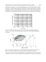
Similar to Sec. 4.1.1, an accuracy analysis of the kinematically redundant 3(P)RPR mechanism
is performed. Exemplarily, simulation results of the three triangular trajectories (t
I

, t
II
, t
III
)
which are shown in Fig. 8 are presented. In the following, facts and definitions similar to the
analysis of the 3(P
)RRR mechanism and already introduced are not mentioned again. Based
on the data sheets of commercially available standard actuators, the active joint errors were
chosen to ∆θ
(3(P)RPR) = (0.2 mm, 0.2 mm, 0.2 mm, 40 µm)
T
. As well, in the non-redundant
case the last element of ∆θ vanishes.
In Fig. 9 the optimized switching patterns δ
opt
of the actuator position δ as well as the resulting
pose errors
∆xy and ∆φ of the mechanisms are presented. Again, the EE was moved counter-
clockwise along trajectory t
I
with a constant orientation of φ = −30
◦
, φ = 0
◦
, and φ = 30
◦
.
It is important to note that the symmetrical non-redundant mechanism suffers from a com-
pletely singular. i.e. useless, workspace for φ

= 0
◦
(indicated by ∆xy = ∆φ = ∞). This is
AdvancesinRobotManipulators394
(a) 3(P)RPR (φ = −30
◦
) (b) 3(P)RPR (φ = 0
◦
) (c) 3(P)RPR (φ = 30
◦
)
Fig. 8. Exemplarily chosen trajectories t
I
, t
II
, t
III
(solid gray) for the 3(P)RPR mechanism,
the solid red lines represent the singularity loci within the workspace (solid black); note: the
workspace for φ
= 0
◦
is completely singular
s
δ [m]
c
I,1
c
I,2
c

I,3
c
I,1
-0.5
-0.3
-0.1
(a) δ
opt
(t
I
(−30
◦
))
s
c
I,1
c
I,2
c
I,3
c
I,
1
(b) δ
opt
(t
I
(0
◦
))

s
c
I,1
c
I,2
c
I,3
c
I,1
(c) δ
opt
(t
I
(30
◦
))
s
∆xy [mm]


c
I,1
c
I,2
c
I,3
c
I,1
0.4
0.7

1
(d) ∆xy(t
I
(−30
◦
))
s
∞
c
I,1
c
I,2
c
I,3
c
I,1
(e) ∆xy(t
I
(0
◦
))
s
c
I,1
c
I,2
c
I,3
c
I,1

(f) ∆xy(t
I
(30
◦
))
s
∆φ [°]


c
I,1
c
I,2
c
I,3
c
I,1
0.1
0.35
0.6
(g) ∆φ(t
I
(−30
◦
))
s
∞
c
I,1
c

I,2
c
I,3
c
I,1
(h) ∆φ(t
I
(0
◦
))
s
c
I,1
c
I,2
c
I,3
c
I,1
(i) ∆φ(t
I
(30
◦
))
Fig. 9. Simulation results while moving along trajectory t
I
(−30
◦
) (left), t
I

(0
◦
) (center), and
t
I
(30
◦
) (right); solid gray: non-redundant mechanism; dashed black: optimized redundant
mechanism using η
(J
h
); solid red: optimized redundant mechanism using γ(∆x
h
)
not the case for the kinematically redundant 3(P)RPR mechanism where the symmetry can be
affected, i.e. avoided, thanks to the additional prismatic actuator. Regarding Fig. 9 and Table 3
similar to the 3R
RR-based structure (see Sec. 4.1.1) a significant improvement of the achiev-
able accuracy due to the kinematic redundancy is well noticeable. Again, in most cases (except
t
i
(φ) Value 3RPR
3(P)RPR
using η
(J
h
) using γ(∆x
h
)
t

I
(−30
◦
)
∆xy
max
[mm] 4.87 0.70 (-85.7%) 0.70 (-85.7%)
∆φ
max
[
◦
] 1.54 0.16 (-89.9%) 0.16 (-89.9%)
t
I
(0
◦
)
∆xy
max
[mm] ∞ 0.90 (-) 0.90 (-)
∆φ
max
[
◦
] ∞ 0.53 (-) 0.48 (-)
t
I
(30
◦
)

∆xy
max
[mm] 0.97 0.66 (-31.8%) 0.66 (-32.5%)
∆φ
max
[
◦
] 0.60 0.35 (-41.1%) 0.32 (-46.6%)
t
II
(−30
◦
)
∆xy
max
[mm] 0.97 0.66 (-31.9%) 0.86 (-11.7%)
∆φ
max
[
◦
] 0.60 0.32 (-46.6%) 0.35 (-41.9%)
t
II
(0
◦
)
∆xy
max
[mm] ∞ 0.91 (-) 0.78 (-)
∆φ

max
[
◦
] ∞ 0.48 (-) 0.44 (-)
t
II
(30
◦
)
∆xy
max
[mm] 4.87 0.70 (-85.7%) 0.64 (-86.8%)
∆φ
max
[
◦
] 1.54 0.16 (-89.9%) 0.15 (-90.2%)
t
III
(−30
◦
)
∆xy
max
[mm] 0.98 0.93 (-4.6%) 0.93 (-4.9%)
∆φ
max
[
◦
] 0.35 0.29 (-17.4%) 0.28 (-21.2%)

t
III
(0
◦
)
∆xy
max
[mm] ∞ ∞ (-) ∞ (-)
∆φ
max
[
◦
] ∞ ∞ (-) ∞ (-)
t
III
(30
◦
)
∆xy
max
[mm] 1.20 0.93 (-22.2%) 0.93 (-22.2%)
∆φ
max
[
◦
] 0.41 0.27 (-34.1%) 0.27 (-34.1%)
Table 3. Redundant 3(P)RPR mechanism: maximal translational ∆xy
max
and rotational error
∆φ

max
of the moving platform while moving along trajectory t
I
, t
II
, and t
III
for t
II
(−30
◦
)) the optimization based on the gain γ(∆x
h
) leads to more appropriate switching
patterns (in terms of accuracy improvement) in comparison to an optimization based on the
Jacobian’s condition η
(J
h
). It is important to note, that even the redundant mechanism suffers
from singularities (see t
III
(0
◦
)). This might be overcome by an optimization of the redundant
actuator’s design which will be subject to future work.
4.1.3 Influence of the redundant actuator’s joint error
An additional test was performed to clarify the influence of the redundant prismatic actua-
tor joint error ∆δ on the moving platform pose error ∆x. Therefore, for different ∆δ the EE
was moved along I(
−30

◦
). The actuator position δ was changed according to the optimized
switching pattern shown in Fig. 7 and Fig. 9 (based on the gain γ
(∆x
h
)). The results are pre-
sented in Fig. 10. The plots clearly demonstrate the marginal influence of ∆δ on ∆x when
realistic values for the remaining active joint errors are chosen (cp. Sec. 4.1.1 and 4.1.2). It can
be seen that even in the case of an unrealistic high joint error ∆δ a significant increase of the
mechanism’s achievable accuracy in comparison to the non-redundant case is still obtained
(cp. Fig. 7, left column).
4.1.4 Switching operations - accuracy progress
There might be the case that the EE passes a singular configuration while performing a re-
configuration of the mechanism, i.e. while changing the singularity loci. As a result, the
performance of the PKM decreases dramatically. Hence, the switching operations have to be
ImprovingthePoseAccuracyofPlanarParallel
RobotsusingMechanismsofVariableGeometry 395
(a) 3(P)RPR (φ = −30
◦
) (b) 3(P)RPR (φ = 0
◦
) (c) 3(P)RPR (φ = 30
◦
)
Fig. 8. Exemplarily chosen trajectories t
I
, t
II
, t
III

(solid gray) for the 3(P)RPR mechanism,
the solid red lines represent the singularity loci within the workspace (solid black); note: the
workspace for φ
= 0
◦
is completely singular
s
δ [m]
c
I,1
c
I,2
c
I,3
c
I,1
-0.5
-0.3
-0.1
(a) δ
opt
(t
I
(−30
◦
))
s
c
I,1
c

I,2
c
I,3
c
I,1
(b) δ
opt
(t
I
(0
◦
))
s
c
I,1
c
I,2
c
I,3
c
I,1
(c) δ
opt
(t
I
(30
◦
))
s
∆xy [mm]



c
I,1
c
I,2
c
I,3
c
I,1
0.4
0.7
1
(d) ∆xy(t
I
(−30
◦
))
s
∞
c
I,1
c
I,2
c
I,3
c
I,1
(e) ∆xy(t
I

(0
◦
))
s
c
I,1
c
I,2
c
I,3
c
I,1
(f) ∆xy(t
I
(30
◦
))
s
∆φ [°]


c
I,1
c
I,2
c
I,3
c
I,1
0.1

0.35
0.6
(g) ∆φ(t
I
(−30
◦
))
s
∞
c
I,1
c
I,2
c
I,3
c
I,1
(h) ∆φ(t
I
(0
◦
))
s
c
I,1
c
I,2
c
I,3
c

I,1
(i) ∆φ(t
I
(30
◦
))
Fig. 9. Simulation results while moving along trajectory t
I
(−30
◦
) (left), t
I
(0
◦
) (center), and
t
I
(30
◦
) (right); solid gray: non-redundant mechanism; dashed black: optimized redundant
mechanism using η
(J
h
); solid red: optimized redundant mechanism using γ(∆x
h
)
not the case for the kinematically redundant 3(P)RPR mechanism where the symmetry can be
affected, i.e. avoided, thanks to the additional prismatic actuator. Regarding Fig. 9 and Table 3
similar to the 3RRR-based structure (see Sec. 4.1.1) a significant improvement of the achiev-
able accuracy due to the kinematic redundancy is well noticeable. Again, in most cases (except

t
i
(φ) Value 3RPR
3(P
)RPR
using η(J
h
) using γ(∆x
h
)
t
I
(−30
◦
)
∆xy
max
[mm] 4.87 0.70 (-85.7%) 0.70 (-85.7%)
∆φ
max
[
◦
] 1.54 0.16 (-89.9%) 0.16 (-89.9%)
t
I
(0
◦
)
∆xy
max

[mm] ∞ 0.90 (-) 0.90 (-)
∆φ
max
[
◦
] ∞ 0.53 (-) 0.48 (-)
t
I
(30
◦
)
∆xy
max
[mm] 0.97 0.66 (-31.8%) 0.66 (-32.5%)
∆φ
max
[
◦
] 0.60 0.35 (-41.1%) 0.32 (-46.6%)
t
II
(−30
◦
)
∆xy
max
[mm] 0.97 0.66 (-31.9%) 0.86 (-11.7%)
∆φ
max
[

◦
] 0.60 0.32 (-46.6%) 0.35 (-41.9%)
t
II
(0
◦
)
∆xy
max
[mm] ∞ 0.91 (-) 0.78 (-)
∆φ
max
[
◦
] ∞ 0.48 (-) 0.44 (-)
t
II
(30
◦
)
∆xy
max
[mm] 4.87 0.70 (-85.7%) 0.64 (-86.8%)
∆φ
max
[
◦
] 1.54 0.16 (-89.9%) 0.15 (-90.2%)
t
III

(−30
◦
)
∆xy
max
[mm] 0.98 0.93 (-4.6%) 0.93 (-4.9%)
∆φ
max
[
◦
] 0.35 0.29 (-17.4%) 0.28 (-21.2%)
t
III
(0
◦
)
∆xy
max
[mm] ∞ ∞ (-) ∞ (-)
∆φ
max
[
◦
] ∞ ∞ (-) ∞ (-)
t
III
(30
◦
)
∆xy

max
[mm] 1.20 0.93 (-22.2%) 0.93 (-22.2%)
∆φ
max
[
◦
] 0.41 0.27 (-34.1%) 0.27 (-34.1%)
Table 3. Redundant 3(P)RPR mechanism: maximal translational ∆xy
max
and rotational error
∆φ
max
of the moving platform while moving along trajectory t
I
, t
II
, and t
III
for t
II
(−30
◦
)) the optimization based on the gain γ(∆x
h
) leads to more appropriate switching
patterns (in terms of accuracy improvement) in comparison to an optimization based on the
Jacobian’s condition η
(J
h
). It is important to note, that even the redundant mechanism suffers

from singularities (see t
III
(0
◦
)). This might be overcome by an optimization of the redundant
actuator’s design which will be subject to future work.
4.1.3 Influence of the redundant actuator’s joint error
An additional test was performed to clarify the influence of the redundant prismatic actua-
tor joint error ∆δ on the moving platform pose error ∆x. Therefore, for different ∆δ the EE
was moved along I(
−30
◦
). The actuator position δ was changed according to the optimized
switching pattern shown in Fig. 7 and Fig. 9 (based on the gain γ
(∆x
h
)). The results are pre-
sented in Fig. 10. The plots clearly demonstrate the marginal influence of ∆δ on ∆x when
realistic values for the remaining active joint errors are chosen (cp. Sec. 4.1.1 and 4.1.2). It can
be seen that even in the case of an unrealistic high joint error ∆δ a significant increase of the
mechanism’s achievable accuracy in comparison to the non-redundant case is still obtained
(cp. Fig. 7, left column).
4.1.4 Switching operations - accuracy progress
There might be the case that the EE passes a singular configuration while performing a re-
configuration of the mechanism, i.e. while changing the singularity loci. As a result, the
performance of the PKM decreases dramatically. Hence, the switching operations have to be
AdvancesinRobotManipulators396
s
∆xy [mm]
c

I,1
c
I,2
c
I,3
c
I,
1
0.5
1
1.5
(a) 3(P)RRR: ∆xy(t
I
(−30
◦
))
s
∆xy [mm]
c
I,1
c
I,2
c
I,3
c
I,1
0.4
0.6
0.8
(b) 3(P)RPR: ∆xy(t

I
(−30
◦
))
s
∆φ [
◦
]
c
I,1
c
I,2
c
I,3
c
I,1
0.05
0.175
0.3
(c) 3(P)RRR: ∆φ(t
I
(−30
◦
))
s
∆φ [
◦
]
c
I,1

c
I,2
c
I,3
c
I,
1
0.1
0.15
0.2
(d) 3(P)RPR: ∆φ(t
I
(−30
◦
))
Fig. 10. Influence of ∆δ on ∆x while moving the EE along trajectory I(−30
◦
) (solid black:
∆δ
= 0µm; solid red: ∆δ = 50 µm; solid gray: ∆δ = 100 µm; solid light gray: ∆δ = 250 µm
considered within the optimization procedure. While performing a reconfiguration (moving
δ while keeping x constant) the possibility of passing any singularities is taken into account.
Additionally, configurations of low performance are avoided. Exemplarily, the behavior of
the achievable accuracy obtained while moving the EE along t
I
(−30
◦
) (including the switch-
ing operations) is given in Fig. 11. It can be clearly seen that the achievable accuracy does
not increase during reconfigurations of the mechanism. This is valid for all the trajectories

the authors tested so far. A problem however is the additional operation time necessary to
follow a desired path. This, i.e. the number of reconfigurations, could be reduced according
to the modifications mentioned in Sec. 3.2, e.g. only change δ once before starting the desired
movement or if the mechanism is unable to perform a desired operation. Furthermore, the
switching time itself could be reduced by a ’semi discrete’ optimization strategy, e.g. start
moving δ shortly before arriving at the ending point c
i,j
of the segment j of trajectory i.
4.2 Comparing the useable workspace
In order to further clarify the effect of an additional prismatic actuator on the mechanism pose
accuracy, in the following, the size of the useable workspaces w
u
is determined. The useable
workspace is defined as the singularity-free part of the total workspace w
t
providing a cer-
tain desired performance, in this case a certain desired accuracy. Mathematically, it can be ex-
pressed as the largest region where the sign of the determinant of the Jacobian det
(A) does not
change and the output error ∆x (23) satisfies any thresholds ∆x
thr
= (∆xy
thr
, ∆φ
thr
)
T
, corre-
sponding to
∆xy and ∆φ. Therefore, the Jacobian determinant as well as the moving platform

pose error are calculated over the whole workspace. An example clarifying the procedure
leading to w
u
is given in Fig. 12. The analyzed workspaces for three different EE orientations
of the non-redundant 3R
RR mechanism (δ = 0 m = const.) is given. The green part is the
largest region where the sign of det
(A) does not change whereas the red part is the smallest.
The black area is the overlayed region where a required performance, i.e. a required accuracy,
s
∆δ [m]∆
∆φ
150
c
I,1
c
I,2
c
I,3
c
I,1
-0.5
0.1
(a) 3(P)RRR: δ
opt
(t
I
(−30
◦
))

s
∆δ [m]∆
∆φ
150
c
I,1
c
I,2
c
I,3
c
I,1
-0.5
-0.2
(b) 3(P)RPR: δ
opt
(t
I
(−30
◦
))
s
∆xy [mm]
∆φ
[°]
100
c
I,1
c
I,2

c
I,3
c
I,1
0.05
0.3
0.5
1.5
(c) 3(P)RRR: ∆xy(t
I
(−30
◦
)), ∆φ(t
I
(−30
◦
))
s
∆xy [mm]
∆φ
[°]
100
c
I,1
c
I,2
c
I,3
c
I,1

0.1
0.2
0.4
0.8
(d) 3(P)RPR: ∆xy(t
I
(−30
◦
)), ∆φ(t
I
(−30
◦
))
Fig. 11. Simulation results (including switching operations) while moving along trajectory
t
I
(−30
◦
), reconfigurations are performed based on the gain; left: 3(P)RRR, right: 3(P)RPR, the
switching operation is marked by the gray background
(a) φ = −30
◦
(b) φ = 0
◦
(c) φ = 30
◦
Fig. 12. Analyzed workspace of the non-redundant 3RRR mechanism (δ = 0m = const.);
green is largest region where the sign of det
(A) does not change whereas red is the smallest,
in the black area the required accuracy can not be provided

can not be provided. Hence, the green color represents the useable workspace with respect to
the mentioned requirements. That followed, the connected green area can be determined, i.e.
the shape as well as the size of the useable workspace.
Three constant EE orientations φ
= {−30
◦
, 0
◦
, 30
◦
} were considered. The design of the ex-
emplarily chosen mechanisms as well as the input error ∆θ are equal to the ones chosen in
Sec. 4.1. The thresholds are set to ∆xy
thr
= 0.75 mm and ∆φ
thr
= 0.5
◦
. The results are given
in Fig. 13. In case of the non-redundant mechanisms the total and useable workspace w
t
and
ImprovingthePoseAccuracyofPlanarParallel
RobotsusingMechanismsofVariableGeometry 397
s
∆xy [mm]
c
I,1
c
I,2

c
I,3
c
I,1
0.5
1
1.5
(a) 3(P)RRR: ∆xy(t
I
(−30
◦
))
s
∆xy [mm]
c
I,1
c
I,2
c
I,3
c
I,1
0.4
0.6
0.8
(b) 3(P)RPR: ∆xy(t
I
(−30
◦
))

s
∆φ [
◦
]
c
I,1
c
I,2
c
I,3
c
I,1
0.05
0.175
0.3
(c) 3(P)RRR: ∆φ(t
I
(−30
◦
))
s
∆φ [
◦
]
c
I,1
c
I,2
c
I,3

c
I,1
0.1
0.15
0.2
(d) 3(P)RPR: ∆φ(t
I
(−30
◦
))
Fig. 10. Influence of ∆δ on ∆x while moving the EE along trajectory I(−30
◦
) (solid black:
∆δ
= 0µm; solid red: ∆δ = 50 µm; solid gray: ∆δ = 100 µm; solid light gray: ∆δ = 250 µm
considered within the optimization procedure. While performing a reconfiguration (moving
δ while keeping x constant) the possibility of passing any singularities is taken into account.
Additionally, configurations of low performance are avoided. Exemplarily, the behavior of
the achievable accuracy obtained while moving the EE along t
I
(−30
◦
) (including the switch-
ing operations) is given in Fig. 11. It can be clearly seen that the achievable accuracy does
not increase during reconfigurations of the mechanism. This is valid for all the trajectories
the authors tested so far. A problem however is the additional operation time necessary to
follow a desired path. This, i.e. the number of reconfigurations, could be reduced according
to the modifications mentioned in Sec. 3.2, e.g. only change δ once before starting the desired
movement or if the mechanism is unable to perform a desired operation. Furthermore, the
switching time itself could be reduced by a ’semi discrete’ optimization strategy, e.g. start

moving δ shortly before arriving at the ending point c
i,j
of the segment j of trajectory i.
4.2 Comparing the useable workspace
In order to further clarify the effect of an additional prismatic actuator on the mechanism pose
accuracy, in the following, the size of the useable workspaces w
u
is determined. The useable
workspace is defined as the singularity-free part of the total workspace w
t
providing a cer-
tain desired performance, in this case a certain desired accuracy. Mathematically, it can be ex-
pressed as the largest region where the sign of the determinant of the Jacobian det
(A) does not
change and the output error ∆x (23) satisfies any thresholds ∆x
thr
= (∆xy
thr
, ∆φ
thr
)
T
, corre-
sponding to ∆xy and ∆φ. Therefore, the Jacobian determinant as well as the moving platform
pose error are calculated over the whole workspace. An example clarifying the procedure
leading to w
u
is given in Fig. 12. The analyzed workspaces for three different EE orientations
of the non-redundant 3RRR mechanism (δ
= 0 m = const.) is given. The green part is the

largest region where the sign of det
(A) does not change whereas the red part is the smallest.
The black area is the overlayed region where a required performance, i.e. a required accuracy,
s
∆δ [m]∆
∆φ
150
c
I,1
c
I,2
c
I,3
c
I,1
-0.5
0.1
(a) 3(P)RRR: δ
opt
(t
I
(−30
◦
))
s
∆δ [m]∆
∆φ
150
c
I,1

c
I,2
c
I,3
c
I,1
-0.5
-0.2
(b) 3(P)RPR: δ
opt
(t
I
(−30
◦
))
s
∆xy [mm]
∆φ
[°]
100
c
I,1
c
I,2
c
I,3
c
I,1
0.05
0.3

0.5
1.5
(c) 3(P)RRR: ∆xy(t
I
(−30
◦
)), ∆φ(t
I
(−30
◦
))
s
∆xy [mm]
∆φ
[°]
100
c
I,1
c
I,2
c
I,3
c
I,1
0.1
0.2
0.4
0.8
(d) 3(P)RPR: ∆xy(t
I

(−30
◦
)), ∆φ(t
I
(−30
◦
))
Fig. 11. Simulation results (including switching operations) while moving along trajectory
t
I
(−30
◦
), reconfigurations are performed based on the gain; left: 3(P)RRR, right: 3(P)RPR, the
switching operation is marked by the gray background
(a) φ = −30
◦
(b) φ = 0
◦
(c) φ = 30
◦
Fig. 12. Analyzed workspace of the non-redundant 3RRR mechanism (δ = 0m = const.);
green is largest region where the sign of det
(A) does not change whereas red is the smallest,
in the black area the required accuracy can not be provided
can not be provided. Hence, the green color represents the useable workspace with respect to
the mentioned requirements. That followed, the connected green area can be determined, i.e.
the shape as well as the size of the useable workspace.
Three constant EE orientations φ
= {−30
◦

, 0
◦
, 30
◦
} were considered. The design of the ex-
emplarily chosen mechanisms as well as the input error ∆θ are equal to the ones chosen in
Sec. 4.1. The thresholds are set to ∆xy
thr
= 0.75 mm and ∆φ
thr
= 0.5
◦
. The results are given
in Fig. 13. In case of the non-redundant mechanisms the total and useable workspace w
t
and
AdvancesinRobotManipulators398
−0.5 0 0.5
0
1
δ [m ]
w
t
, w
u
[m
2
]
(a) 3(P)RRR: φ = −30
◦

−0.5 0 0.5
0
1
δ [m ]
w
t
, w
u
[m
2
]
(b) 3(P)RPR: φ = −30
◦
−0.5 0 0.5
0
1
δ [m ]
w
t
, w
u
[m
2
]
(c) 3(P)RRR: φ = 0
◦
−0.5 0 0.5
0
1
δ [m ]

w
t
, w
u
[m
2
]
(d) 3(P)RPR: φ = 0
◦
−0.5 0 0.5
0
1
δ [m ]
w
t
, w
u
[m
2
]
(e) 3(P)RRR: φ = 30
◦
−0.5 0 0.5
0
1
δ [m ]
w
t
, w
u

[m
2
]
(f) 3(P)RPR: φ = 30
◦
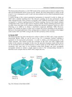
Fig. 13. Total (bold lines, filled dots) and useable (light lines, unfilled dots) workspace of the
kinematically redundant 3(P
)RRR mechanism (left, solid red), the 3(P)RPR mechanism (right,
solid red), and their non-redundant counterparts (left/right, dotted blue); the dashed red line
gives the useable workspace of the redundant mechanisms for ∆x
thr
= (0.5mm, 0.35
◦
)
T
w
u
was calculated for different base joint positions G
1
i
, i.e. for different but constant δ
i
. The
solid horizontal lines represent w
t
and w
u
for the redundant case when the base joint G
1
can

be moved linearly for
−0.5 m ≤ δ ≤ 0.5 m. Having a look at Fig. 13 a significant improve-
ment concerning the workspace areas for all the considered EE orientations is well noticeable.
Furthermore, for the redundant case the useable workspace for ∆x
thr
= (0.5 mm, 0.35
◦
)
T
was determined, i.e. the requested accuracy is increased about one third. It can be clearly
seen that in this case similar workspace sizes are obtained in comparison the non-redundant
mechanisms with less accuracy requirements. This further demonstrates the use of kinematic
redundancy in terms of accuracy improvements.
5. Conclusion
In this paper, the kinematically redundant 3(P)RRR and 3(P)RPR mechanisms were presented.
In each case, an additional prismatic actuator was applied to the structure allowing one base
joint to move linearly. After a description of some fundamentals of the proposed PKM, the
effect of the additional DOF on the moving platform pose accuracy was clarified. An opti-
mization of the redundant actuator position in a discrete manner was introduced. It is based
on a minimization of a criterion that the authors denoted the gain γ
(∆x
h
) of the maximal
homogenized pose error ∆x
h
. Using several exemplarily chosen trajectories a significant im-
provement in terms of accuracy of the proposed redundant mechanisms in combination with
the developed optimization procedure was demonstrated. It could be seen that the suggested
index γ
(∆x

h
) leads to more appropriate switching patterns than the well known condition
number of the Jacobian. Additional simulations demonstrated the marginal influence of the
redundant actuator joint error ∆δ on the moving platform pose error ∆x.
Furthermore, a comparative study on the usable workspaces, i.e. the singularity-free part of
the total workspace providing a certain desired performance, of the mentioned mechanisms
and their non-redundant counterparts was performed. The results demonstrate a significant
increase of the useable workspace of all considered EE orientations thanks to the applied ad-
ditional prismatic actuator.
To further increase the overall and the operational workspace, future work will deal with the
design optimization of the prismatic actuator, e.g. its orientation with respect to the x-axis of
the inertial coordinate frame as well as its stroke (’length’). In addition, the simulation will be
extended to PKM with higher DOF and an experimental validation of the obtained numerical
results will be performed.
6. References
Arakelian, V., Briot, S. & Glazunov, V. (2008). Increase of singularity-free zones in the
workspace of parallel manipulators using mechanisms of variable structure, Mech
Mach Theory 43(9): 1129–1140.
Cha, S H., Lasky, T. A. & Velinsky, S. A. (2007). Singularity avoidance for the 3-RRR mech-
anism using kinematic redundancy, Proc. of the 2007 IEEE International Conference on
Robotics and Automation, pp. 1195–1200.
Ebrahimi, I., Carretero, J. A. & Boudreau, R. (2007). 3-PRRR redundant planar parallel ma-
nipulator: Inverse displacement, workspace and singularity analyses, Mechanism &
Machine Theory 42(8): 1007–1016.
Gosselin, C. M. (1992). Optimum design of robotic manipulators using dexterity indices,
Robotics and Autonomous Systems 9(4): 213–226.
Gosselin, C. M. & Angeles, J. (1988). The optimum kinematic design of a planar three-degree-
of-freedom parallel manipulator, Journal of Mechanisms, Transmissions, and Automation
in Design 110(1): 35–41.
Gosselin, C. M. & Angeles, J. (1990). Singularity analysis of closed-loop kinematic chains, IEEE

Transactions on Robotics and Automation 6(3): 281–290.
Hunt, K. H. (1978). Kinematic Geometry of Mechanisms, Clarendon Press.
Kock, S. (2001). Parallelroboter mit Antriebsredundanz, PhD thesis, Institute of Control Engineer-
ing, TU Brunswick, Germany.
ImprovingthePoseAccuracyofPlanarParallel
RobotsusingMechanismsofVariableGeometry 399
−0.5 0 0.5
0
1
δ [m ]
w
t
, w
u
[m
2
]
(a) 3(P)RRR: φ = −30
◦
−0.5 0 0.5
0
1
δ [m ]
w
t
, w
u
[m
2
]

(b) 3(P)RPR: φ = −30
◦
−0.5 0 0.5
0
1
δ [m ]
w
t
, w
u
[m
2
]
(c) 3(P)RRR: φ = 0
◦
−0.5 0 0.5
0
1
δ [m ]
w
t
, w
u
[m
2
]
(d) 3(P)RPR: φ = 0
◦
−0.5 0 0.5
0

1
δ [m ]
w
t
, w
u
[m
2
]
(e) 3(P)RRR: φ = 30
◦
−0.5 0 0.5
0
1
δ [m ]
w
t
, w
u
[m
2
]
(f) 3(P)RPR: φ = 30
◦
Fig. 13. Total (bold lines, filled dots) and useable (light lines, unfilled dots) workspace of the
kinematically redundant 3(P)RRR mechanism (left, solid red), the 3(P)RPR mechanism (right,
solid red), and their non-redundant counterparts (left/right, dotted blue); the dashed red line
gives the useable workspace of the redundant mechanisms for ∆x
thr
= (0.5mm, 0.35

◦
)
T
w
u
was calculated for different base joint positions G
1
i
, i.e. for different but constant δ
i
. The
solid horizontal lines represent w
t
and w
u
for the redundant case when the base joint G
1
can
be moved linearly for
−0.5 m ≤ δ ≤ 0.5 m. Having a look at Fig. 13 a significant improve-
ment concerning the workspace areas for all the considered EE orientations is well noticeable.
Furthermore, for the redundant case the useable workspace for ∆x
thr
= (0.5 mm, 0.35
◦
)
T
was determined, i.e. the requested accuracy is increased about one third. It can be clearly
seen that in this case similar workspace sizes are obtained in comparison the non-redundant
mechanisms with less accuracy requirements. This further demonstrates the use of kinematic

redundancy in terms of accuracy improvements.
5. Conclusion
In this paper, the kinematically redundant 3(P)RRR and 3(P)RPR mechanisms were presented.
In each case, an additional prismatic actuator was applied to the structure allowing one base
joint to move linearly. After a description of some fundamentals of the proposed PKM, the
effect of the additional DOF on the moving platform pose accuracy was clarified. An opti-
mization of the redundant actuator position in a discrete manner was introduced. It is based
on a minimization of a criterion that the authors denoted the gain γ
(∆x
h
) of the maximal
homogenized pose error
∆x
h
. Using several exemplarily chosen trajectories a significant im-
provement in terms of accuracy of the proposed redundant mechanisms in combination with
the developed optimization procedure was demonstrated. It could be seen that the suggested
index γ
(∆x
h
) leads to more appropriate switching patterns than the well known condition
number of the Jacobian. Additional simulations demonstrated the marginal influence of the
redundant actuator joint error ∆δ on the moving platform pose error ∆x.
Furthermore, a comparative study on the usable workspaces, i.e. the singularity-free part of
the total workspace providing a certain desired performance, of the mentioned mechanisms
and their non-redundant counterparts was performed. The results demonstrate a significant
increase of the useable workspace of all considered EE orientations thanks to the applied ad-
ditional prismatic actuator.
To further increase the overall and the operational workspace, future work will deal with the
design optimization of the prismatic actuator, e.g. its orientation with respect to the x-axis of

the inertial coordinate frame as well as its stroke (’length’). In addition, the simulation will be
extended to PKM with higher DOF and an experimental validation of the obtained numerical
results will be performed.
6. References
Arakelian, V., Briot, S. & Glazunov, V. (2008). Increase of singularity-free zones in the
workspace of parallel manipulators using mechanisms of variable structure, Mech
Mach Theory 43(9): 1129–1140.
Cha, S H., Lasky, T. A. & Velinsky, S. A. (2007). Singularity avoidance for the 3-RRR mech-
anism using kinematic redundancy, Proc. of the 2007 IEEE International Conference on
Robotics and Automation, pp. 1195–1200.
Ebrahimi, I., Carretero, J. A. & Boudreau, R. (2007). 3-P
RRR redundant planar parallel ma-
nipulator: Inverse displacement, workspace and singularity analyses, Mechanism &
Machine Theory 42(8): 1007–1016.
Gosselin, C. M. (1992). Optimum design of robotic manipulators using dexterity indices,
Robotics and Autonomous Systems 9(4): 213–226.
Gosselin, C. M. & Angeles, J. (1988). The optimum kinematic design of a planar three-degree-
of-freedom parallel manipulator, Journal of Mechanisms, Transmissions, and Automation
in Design 110(1): 35–41.
Gosselin, C. M. & Angeles, J. (1990). Singularity analysis of closed-loop kinematic chains, IEEE
Transactions on Robotics and Automation 6(3): 281–290.
Hunt, K. H. (1978). Kinematic Geometry of Mechanisms, Clarendon Press.
Kock, S. (2001). Parallelroboter mit Antriebsredundanz, PhD thesis, Institute of Control Engineer-
ing, TU Brunswick, Germany.
AdvancesinRobotManipulators400
Kock, S. & Schumacher, W. (1998). A parallel x-y manipulator with actuation redundancy
for high-speed and active-stiffness applications, Proc. of the 1998 IEEE International
Conference on Robotics and Automation, pp. 2295–2300.
Kotlarski, J., Abdellatif, H. & Heimann, B. (2007). On singularity avoidance and workspace
enlargement of planar parallel manipulators using kinematic redundancy, Proc. of the

13th IASTED International Conference on Robotics and Applications, pp. 451–456.
Kotlarski, J., Abdellatif, H. & Heimann, B. (2008). Improving the pose accuracy of a planar
3R
RR parallel manipulator using kinematic redundancy and optimized switching
patterns, Proc. of the 2008 IEEE International Conference on Robotics and Automation,
Pasadena, USA, pp. 3863–3868.
Kotlarski, J., Abdellatif, H., Ortmaier, T. & Heimann, B. (2009). Enlarging the useable
workspace of planar parallel robots using mechanisms of variable geometry, Proc.
of the ASME/IFToMM International Conference on Reconfigurable Mechanisms and Robots,
London, United Kingdom, pp. 94–103.
Kotlarski, J., de Nijs, R., Abdellatif, H. & Heimann, B. (2009). New interval-based approach
to determine the guaranteed singularity-free workspace of parallel robots, Proc. of the
2009 International Conference on Robotics and Automation, Kobe, Japan, pp. 1256–1261.
Kotlarski, J., Do Thanh, T., Abdellatif, H. & Heimann, B. (2008). Singularity avoidance of a
kinematically redundant parallel robot by a constrained optimization of the actua-
tion forces, Proc. of the 17th CISM-IFToMM Symposium on Robot Design, Dynamics, and
Control, Tokyo, Japan, pp. 435–442.
Merlet, J P. (1996). Redundant parallel manipulators, Laboratory Robotics and Automation
8(1): 17–24.
Merlet, J P. (2006a). Computing the worst case accuracy of a pkm over a workspace or a
trajectory, Proc. of the 5th Chemnitz Parallel Kinematics Seminar, pp. 83–96.
Merlet, J P. (2006b). Parallel Robots (Second Edition), Springer.
Merlet, J P. & Daney, D. (2005). Dimensional synthesis of parallel robots with a guaranteed
given accuracy over a specific workspace, Proc. of the 2005 IEEE International Confer-
ence on Robotics and Automation, pp. 942–947.
Mohamed, M. G. & Gosselin, C. M. (2005). Design and analysis of kinematically redun-
dant parallel manipulators with configurable platforms, IEEE Transactions on Robotics
21(3): 277–287.
Müller, A. (2005). Internal preload control of redundantly actuated parallel manipulators & its
application to backlash avoiding control, IEEE Transactions on Robotics and Automation

21(4): 668–677.
Pond, G. & Carretero, J. A. (2006). Formulating jacobian matrices for the dexterity analysis of
parallel manipulators, Mechanism & Machine Theory 41(12): 1505–1519.
Wang, J. & Gosselin, C. M. (2004). Kinematic analysis and design of kinematically redundant
parallel mechanisms, Journal of Mechanical Design 126(1): 109–118.
Yang, G., Chen, W. & Chen, I M. (2002). A geometrical method for the singularity analysis of
3-RRR planar parallel robots with different actuation schemes, Pro. of the 2002 IEEE
International Conference on Intelligent Robots and Systems, pp. 2055–2060.
Zein, M., Wenger, P. & Chablat, D. (2006). Singular curves and cusp points in the joint space of
3-RPR parallel manipulators, Proc. of the 2006 IEEE International Conference on Robotics
and Automation, pp. 777–782.
KinematicSingularitiesofRobotManipulators 401
KinematicSingularitiesofRobotManipulators
PeterDonelan
0
Kinematic Singularities
of Robot Manipulators
Peter Donelan
Victoria University of Wellington
New Zealand
1. Introduction
Kinematic singularities of robot manipulators are configurations in which there is a change in
the expected or typical number of instantaneous degrees of freedom. This idea can be made
precise in terms of the rank of a Jacobian matrix relating the rates of change of input (joint)
and output (end-effector position) variables. The presence of singularities in a manipulator’s
effective joint space or work space can profoundly affect the performance and control of the
manipulator, variously resulting in intolerable torques or forces on the links, loss of stiffness
or compliance, and breakdown of control algorithms. The analysis of kinematic singularities
is therefore an essential step in manipulator design. While, in many cases, this is motivated
by a desire to avoid singularities, it is known that for almost all manipulator architectures,

the theoretical joint space must contain singularities. In some cases there are potential design
advantages in their presence, for example fine control, increased load-bearing and singularity-
free posture change.
There are several distinct aspects to singularity analysis—in any given problem it may only
be necessary to address some of them. Starting with a given manipulator architecture, ma-
nipulator kinematics describe the relation between the position and velocity (instantaneous
or infinitesimal kinematics) of the joints and of the end-effector or platform. The physical
construction and intended use of the manipulator are likely to impose constraints on both the
input and output variables; however, it may be preferable to ignore such constraints in an
initial analysis in order to deduce subsequently joint and work spaces with desirable charac-
teristics. A common goal is to determine maximal singularity-free regions. Hence, there is
a global problem to determine the whole locus of singular configurations. Depending on the
architecture, one may be interested in the singular locus in the joint space or in the work space
of the end-effector (or both). A more detailed problem is to classify the types of singularity
within the critical locus and thereby to stratify the locus. A local problem is to determine the
structure of the singular locus in the neighbourhood of a particular point. For example, it may
be important to know whether the locus separates the space into distinct subsets, a strong
converse to this being that a singular configuration is isolated.
Typically, there will be a number of design parameters for a manipulator with given
architecture—link lengths, twists and offsets. Bifurcation analysis concerns the changes in
both local and global structure of the singular locus that occur as one alters design param-
eters in a given architecture. The design process is likely to involve optimizing some desired
characteristic(s) with respect to the design parameters.
20
AdvancesinRobotManipulators402
The aim of this Chapter is to provide an overview of the development and current state of
kinematic singularity research and to survey some of the specific methodology and results
in the literature. More particularly, it describes a framework, based on the work of Müller
(2006; 2009) and of the author (Donelan, 2007b; 2008), in which singularities of both serial and
parallel manipulators can be understood.

2. Origins and Development
The origins of the the study of singularities in mechanism and machine research literature go
back to the 1960s and relate particularly to determination of the degree of mobility via screw
theory (Baker, 1978; Waldron, 1966), the study of over-constrained closed chains (Duffy &
Gilmartin, 1969) and the analysis of inverse kinematics for serial manipulators. Pieper (1968)
showed that the inverse kinematic problem could be solved explicitly for wrist-partitioned
manipulators, typical among serial manipulator designs. Generally, this remains a major
problem in manipulator kinematics and singularity analysis. In the context of control meth-
ods, Whitney introduced the Jacobian matrix (Whitney, 1969) and this has become the central
object in the study of instantaneous kinematics of manipulators and their singularities—a
number of significant articles appeared in the succeeding years (Featherstone, 1982; Litvin et
al., 1986; Paul & Shimano, 1978; Sugimoto et al., 1982; Waldron, 1982; Waldron et al., 1985);
now the literature on kinematic singularities is very extensive, numbering well over a thou-
sand items.
Interest in parallel mechanisms also gained momentum in the 1980s. Hunt (1978) proposed
the use of in-parallel actuated mechanisms, such as the Gough–Stewart platform (Dasgupta &
Mruthyunjaya, 2000), as robot manipulators, given their advantages of stiffness and precision.
In contrast to serial manipulators, where the forward kinematic mapping is constructible and
its singularities correspond to a loss of degrees of freedom in the end-effector, for parallel ma-
nipulators, the inverse kinematics is generally more tractable and its singularities correspond
to a gain in freedom for the platform or end-effector (Fichter, 1986; Hunt, 1983). While screw
theory already played a role in analyzing singularities, Merlet (1989) showed that Grassmann
line geometry, which could be viewed as a subset of screw theory (see Section 4.2), is suffi-
ciently powerful to explain the singular configurations of the Gough–Stewart platform. There-
after, a Jacobian-based approach to understanding parallel manipulator singularities was pro-
vided by Gosselin & Angeles (1990), who showed that they could experience both direct and
inverse kinematic singularities and indeed a combination of these. Subsequently, the sub-
tlety of parallel manipulator kinematics has become even more apparent, in part as a result of
the development of manipulators with restricted types of mobility, such as translational and
Schönflies manipulators (Carricato, 2005; Di Gregorio & Parenti-Castelli, 2002).

The difficulty in resolving the precise configuration space and singularity locus have meant
that a great deal of the singularity analysis takes a localized approach—one assumes a given
configuration for the manipulator and then determines whether it is a singular configuration.
It may also bepossible to determine somelocal characteristics of the locus of singularities. This
is remarkably fruitful: by choosing coordinates so that the given configuration is the identity
or home configuration it is possible to reason about necessary conditions for singularity in
terms of screws and screw systems. The difficulty that arises in deducing the global structure
of the singularity locus is that there is no straightforward way to solve the necessary inverse
kinematics. A good deal of progress can be made in some problems using Lie algebra and
properties of the closure subalgebra of a chain (open or closed). This approach can be found
in (Hao, 1998; Rico et al., 2003) but it appears to fail for the mechanisms dubbed “paradoxical"
by Hervé (1978).
A number of authors have sought to apply methods of mathematical singularity theory to the
study of manipulator singularities, for example Gibson (1992); Karger (1996); Pai & Leu (1992);
Tcho´n (1991). A recent survey of this approach can be found in (Donelan, 2007b). There are
several salient features. Firstly, the kinematic mapping is explicitly recognized as a function
between manifolds, though it may not be given explicit form. Secondly, singularities may be
classified not only on the basis of their kinematic status but also in terms of intrinsic character-
istics of the mapping. For example, the rank deficiency (corank) of the kinematic mapping is a
simple discriminator. More subtle higher-order distinctions can be made that distinguish be-
tween the topological types of the local singularity locus and enable it to be stratified. Thirdly,
it provides a precise language and machinery for determining generic properties of the kine-
matics.
Following the results of Merlet (1989), another approach has been to use geometric algebra,
especially in the analysis of parallel manipulator kinematics and singularities. It is a common
theme that singular configurations correspond to special configurations of points, lines and
planes associated with a manipulator—for example coplanarity of joint axes or collinearity
of spherical joints. Such conditions can be expressed as simple equations in the appropriate
algebra. Some examples of recent successful application of these techniques are Ben-Horin &
Shoham (2009); Torras et al. (1996); White (1994); Wolf et al. (2004).

3. Manipulator Architecture and Mobility
A robot manipulator is assumed to consist of a number of rigid components (links), some pairs
of which are connected by joints that are assumed to be Reuleaux lower pairs, so representable
by the contact of congruent surfaces in the connected pair of links (Hunt, 1978). These include
three types with one degree of freedom (dof): revolute R, prismatic P and helical or screw H
(the first two correspond to purely rotational and purely translational freedom respectively)
and three types having higher degree of freedom: cylindrical C with 2 dof, planar E and
spherical S each with 3 dof. Some manipulators include universal U joints consisting of two R
joints with intersecting axes, also denoted (RR).
The architecture of a manipulator is essentially a topological description of its links and joints:
it can be determined by a graph whose vertices are the links and whose edges represent joints
(Müller, 2006). A serial manipulator is an open chain consisting of a sequence of pairwise joined
links, the initial (base) and final (end-effector) links only being connected to one other link.
If the initial and final links of a serial manipulator are connected to each other, the result is a
simple closed chain. This is the most basic example of a parallel manipulator, that is a manipulator
whose topological representation includes at least one cycle or loop. Note that manipulators
such as multi-fingered robot hands are neither serial nor parallel—their graph is a tree and
the relevant kinematics are likely to concern the simultaneous placement of each finger.
Associated with the architecture is a combinatorial invariant, the (full-cycle) mobility µ of the
manipulator, which is its total internal or relative number of degrees of freedom. This is given
by the formula of Chebychev–Grübler–Kutzbach (CGK) (Hunt, 1978; Waldron, 1966):
µ
= n(l −1) −
k
∑
i=1
(n −δ
i
) =
k

∑
i=1
δ
i
−n(k −l + 1) (1)
where n is the number of degrees of freedom of an unconstrained link (n
= 6 for spatial, n = 3
for planar or spherical manipulators), k is the number of joints, l the number of links and δ
i
the
KinematicSingularitiesofRobotManipulators 403
The aim of this Chapter is to provide an overview of the development and current state of
kinematic singularity research and to survey some of the specific methodology and results
in the literature. More particularly, it describes a framework, based on the work of Müller
(2006; 2009) and of the author (Donelan, 2007b; 2008), in which singularities of both serial and
parallel manipulators can be understood.
2. Origins and Development
The origins of the the study of singularities in mechanism and machine research literature go
back to the 1960s and relate particularly to determination of the degree of mobility via screw
theory (Baker, 1978; Waldron, 1966), the study of over-constrained closed chains (Duffy &
Gilmartin, 1969) and the analysis of inverse kinematics for serial manipulators. Pieper (1968)
showed that the inverse kinematic problem could be solved explicitly for wrist-partitioned
manipulators, typical among serial manipulator designs. Generally, this remains a major
problem in manipulator kinematics and singularity analysis. In the context of control meth-
ods, Whitney introduced the Jacobian matrix (Whitney, 1969) and this has become the central
object in the study of instantaneous kinematics of manipulators and their singularities—a
number of significant articles appeared in the succeeding years (Featherstone, 1982; Litvin et
al., 1986; Paul & Shimano, 1978; Sugimoto et al., 1982; Waldron, 1982; Waldron et al., 1985);
now the literature on kinematic singularities is very extensive, numbering well over a thou-
sand items.

Interest in parallel mechanisms also gained momentum in the 1980s. Hunt (1978) proposed
the use of in-parallel actuated mechanisms, such as the Gough–Stewart platform (Dasgupta &
Mruthyunjaya, 2000), as robot manipulators, given their advantages of stiffness and precision.
In contrast to serial manipulators, where the forward kinematic mapping is constructible and
its singularities correspond to a loss of degrees of freedom in the end-effector, for parallel ma-
nipulators, the inverse kinematics is generally more tractable and its singularities correspond
to a gain in freedom for the platform or end-effector (Fichter, 1986; Hunt, 1983). While screw
theory already played a role in analyzing singularities, Merlet (1989) showed that Grassmann
line geometry, which could be viewed as a subset of screw theory (see Section 4.2), is suffi-
ciently powerful to explain the singular configurations of the Gough–Stewart platform. There-
after, a Jacobian-based approach to understanding parallel manipulator singularities was pro-
vided by Gosselin & Angeles (1990), who showed that they could experience both direct and
inverse kinematic singularities and indeed a combination of these. Subsequently, the sub-
tlety of parallel manipulator kinematics has become even more apparent, in part as a result of
the development of manipulators with restricted types of mobility, such as translational and
Schönflies manipulators (Carricato, 2005; Di Gregorio & Parenti-Castelli, 2002).
The difficulty in resolving the precise configuration space and singularity locus have meant
that a great deal of the singularity analysis takes a localized approach—one assumes a given
configuration for the manipulator and then determines whether it is a singular configuration.
It may also bepossible to determine somelocal characteristics of the locus of singularities. This
is remarkably fruitful: by choosing coordinates so that the given configuration is the identity
or home configuration it is possible to reason about necessary conditions for singularity in
terms of screws and screw systems. The difficulty that arises in deducing the global structure
of the singularity locus is that there is no straightforward way to solve the necessary inverse
kinematics. A good deal of progress can be made in some problems using Lie algebra and
properties of the closure subalgebra of a chain (open or closed). This approach can be found
in (Hao, 1998; Rico et al., 2003) but it appears to fail for the mechanisms dubbed “paradoxical"
by Hervé (1978).
A number of authors have sought to apply methods of mathematical singularity theory to the
study of manipulator singularities, for example Gibson (1992); Karger (1996); Pai & Leu (1992);

Tcho´n (1991). A recent survey of this approach can be found in (Donelan, 2007b). There are
several salient features. Firstly, the kinematic mapping is explicitly recognized as a function
between manifolds, though it may not be given explicit form. Secondly, singularities may be
classified not only on the basis of their kinematic status but also in terms of intrinsic character-
istics of the mapping. For example, the rank deficiency (corank) of the kinematic mapping is a
simple discriminator. More subtle higher-order distinctions can be made that distinguish be-
tween the topological types of the local singularity locus and enable it to be stratified. Thirdly,
it provides a precise language and machinery for determining generic properties of the kine-
matics.
Following the results of Merlet (1989), another approach has been to use geometric algebra,
especially in the analysis of parallel manipulator kinematics and singularities. It is a common
theme that singular configurations correspond to special configurations of points, lines and
planes associated with a manipulator—for example coplanarity of joint axes or collinearity
of spherical joints. Such conditions can be expressed as simple equations in the appropriate
algebra. Some examples of recent successful application of these techniques are Ben-Horin &
Shoham (2009); Torras et al. (1996); White (1994); Wolf et al. (2004).
3. Manipulator Architecture and Mobility
A robot manipulator is assumed to consist of a number of rigid components (links), some pairs
of which are connected by joints that are assumed to be Reuleaux lower pairs, so representable
by the contact of congruent surfaces in the connected pair of links (Hunt, 1978). These include
three types with one degree of freedom (dof): revolute R, prismatic P and helical or screw H
(the first two correspond to purely rotational and purely translational freedom respectively)
and three types having higher degree of freedom: cylindrical C with 2 dof, planar E and
spherical S each with 3 dof. Some manipulators include universal U joints consisting of two R
joints with intersecting axes, also denoted (RR).
The architecture of a manipulator is essentially a topological description of its links and joints:
it can be determined by a graph whose vertices are the links and whose edges represent joints
(Müller, 2006). A serial manipulator is an open chain consisting of a sequence of pairwise joined
links, the initial (base) and final (end-effector) links only being connected to one other link.
If the initial and final links of a serial manipulator are connected to each other, the result is a

simple closed chain. This is the most basic example of a parallel manipulator, that is a manipulator
whose topological representation includes at least one cycle or loop. Note that manipulators
such as multi-fingered robot hands are neither serial nor parallel—their graph is a tree and
the relevant kinematics are likely to concern the simultaneous placement of each finger.
Associated with the architecture is a combinatorial invariant, the (full-cycle) mobility µ of the
manipulator, which is its total internal or relative number of degrees of freedom. This is given
by the formula of Chebychev–Grübler–Kutzbach (CGK) (Hunt, 1978; Waldron, 1966):
µ
= n(l −1) −
k
∑
i=1
(n −δ
i
) =
k
∑
i=1
δ
i
−n(k −l + 1) (1)
where n is the number of degrees of freedom of an unconstrained link (n
= 6 for spatial, n = 3
for planar or spherical manipulators), k is the number of joints, l the number of links and δ
i
the
AdvancesinRobotManipulators404
dofs of the i th joint. The first expression represents the difference between the total freedom
of the links and the constraints imposed by the joints. The second version emphasizes that
the mobility is the difference between the total joint dofs and the number of constraints as

expressed by the dimension of the cycle space of the associated graph (Gross & Yellen, 2004).
A specific manipulator requires more information, determining the variable design parame-
ters inherent in the architecture. The formula (1) is generic (Müller, 2009): there may be specific
realizations of an architecture for which the formula does not give the true mobility. For ex-
ample, the Bennett mechanism consists of 4 links connected by 4 revolute joints into a closed
chain and is designed so that the axes lie pairwise on the two sets of generators of a hyper-
boloid. The CGK formula gives µ
= 6×(4 −1) −
∑
4
i
=1
(6 −1) = −2 but in fact the mechanism
is mobile with 1 dof. Instances of an architecture in which (1) underestimates the true mobil-
ity are termed over-constrained. In other cases, there are specific configurations in which µ
does not coincide with the infinitesimal freedom of the manipulator. This has given rise to
a search for a more universal formula that takes into account the non-generic cases, see for
example (Gogu, 2005). It is precisely the discrepancies that arise which correspond to forms
of singularity that are explored in subsequent sections.
4. The Kinematic Mapping
In the robotics literature, the Jacobian matrix for a serial manipulator is the linear transfor-
mation that relates joint velocities to end-effector velocities. Explicitly, suppose the joint
variables are q
= (q
1
, . . . , q
k
) and the end-effector’s position is described by coordinates
x
= (x

1
, . . . , x
n
). Thus, k is the total number of the joints (or total degrees of freedom, if
any have
≥ 2 dof) of the joints, while n is the dimension of the displacement space of the
end-effector, typically either n
= 3 for planar or spherical motion or n = 6 for full spatial
motion. The kinematic mapping is a function x
= f (θ) that determines the displacement of the
end-effector corresponding to given values of the joint variables. Then for a time-dependent
motion described by q
= q(t), at a configuration q
0
= q(t
0
) say,
˙
x
(t
0
) = J f (q
0
)
˙
q
(t
0
) (2)
where J

= J f (q
0
) is the n ×k matrix of partial derivatives of f with ijth entry ∂ f
i
/∂q
j
. It is
important to note that the linear relation expressed by (2) holds infinitesimally; the Jacobian
matrix is itself dependent on the joint variables. In many practical situations, for example in
control algorithms, the requirement is to find an inverse matrix for J, which is only possible
when k
= n and the determinant of the Jacobian is non-zero. In the case k > n, the kinematics
are said to be redundant and one may seek a pseudo-inverse. In the case of wrist-partitioned
serial manipulators, the Jacobian itself partitions in a natural way and so the singularity loci
of such manipulators can also be analyzed relatively simply (Stani
˘
si´c & Engleberth, 1978). It
is not essential to consider the time-dependence of a motion: from the point of view of the
manipulator’s capabilities, the Jacobian is determined by the choice of coordinates for joints
and end-effector so the properties of interest are those that are invariant under change of
coordinates. This is made clearer if the domain and range of the kinematic mapping f are
properly defined.
4.1 Displacement groups
The range is the set of rigid displacements of the end-effector. The rigidity of the links of
a manipulator, including its end-effector, means that their motion in space is assumed to be
isometric (distance between any pair of points is preserved) and orientation-preserving. As-
suming the ambient space to be Euclidean, the resulting set of possible displacements is the
spatial Euclidean (isometry) group SE
(3) (Murray et al., 1994; Selig, 2005). Composition of dis-
placements and the existence of an inverse displacement ensure that, mathematically, this set

is a group. Moreover it can be, at least on a neighbourhood of every point, given Euclidean
coordinates, and hence forms a Lie group having compatible spatial or topological (differen-
tiable manifold) and algebraic (group) structures. The number of independent coordinates
required is the dimension of the Lie group and SE
(3) is 6-dimensional. It is, via choices of an
origin and 3-dimensional orthonormal coordinates in the ambient space and in the link, iso-
morphic (that isto saytopologically and algebraically equivalent to) to the semi-direct product
SO
(3)  R
3
, where the components of the product correspond to the orientation-preserving
rotations about a fixed point (the origin) and translations, respectively.
For planar manipulators, analogously, the Euclidean isometry group is the 3–dimensional
group SE
(2)
∼
=
SO(2)  R
2
. Every element of the rotation group SO(2) may be written, with
respect to given orthonormal basis for R
2
, in the form:

cos θ
−sin θ
sin θ cos θ

(3)
where θ measures the angle of counter-clockwise rotation. In this case, θ is a coordinate for

the 1-dimensional group SO
(2) which can, in fact, be used globally, though it is not one-to-
one. Indeed, it is clear that SO
(2) is, in a topological sense, the same as a unit circle, denoted
S
1
and θ and θ + 2pπ represent the same point for any integer p. Topologically, SO(3) is
3-dimensional projective space. Coordinates may be chosen in a number of ways. The dimen-
sions correspond locally to the rotation about each of three perpendicular axes, or one can use
Euler angles. Alternatively, there is a 2:1 representation by points of a 3-dimensional sphere,
and unit quaternions or Euler–Rodrigues parameters are often used.
Regarding the joint variables, the motion associated with each Reuleaux pair corresponds to a
subgroup of SE
(3) of the same dimension as its degrees of freedom (Hervé, 1978). In particular
R, P and H joints can be represented by one-dimensional subgroups of the Euclidean group.
For an R joint, the subgroup is topologically S
1
, while for P and H joints the group is R. For
an S joint, the subgroup is (a copy of) SO
(3); for C and E joints the subgroups are equivalent
to S
1
×R and R ×R respectively. Depending on the architecture of the manipulator, its joint
variables therefore lie in a product of components, each of the form either S
1
, R or SO(3), and
this product Q, say, forms the theoretical domain of the kinematic mapping. As mentioned
previously, however, there are in practice almost certainly restrictions on the joint variables
so that the actual domain is some subset of the theoretical joint space. The set Q is also a
manifold for which the joint variables give coordinates, say q

= (q
1
, . . . , q
k
), at least locally
though not necessarily in a one-to-one manner for the whole space at once.
The kinematic mapping has the form of a function f : Q
→ G, where Q is the joint space and
G the displacement group for the end-effector, are well-defined manifolds. Local coordinates
enable f to be expressed explicitly as a formula. While G is usually taken to be SE
(3), for
spherical manipulators in which there is a fixed point for the end-effector G
= SO(3). For a
robot hand or multi-legged walking robot, G may be a product of several copies of SE
(3). For
a positional manipulator, for example a 3R arm assembly that determines the wrist-centre for
a wrist-partitioned serial manipulator, the range is simply R
3
.
KinematicSingularitiesofRobotManipulators 405
dofs of the i th joint. The first expression represents the difference between the total freedom
of the links and the constraints imposed by the joints. The second version emphasizes that
the mobility is the difference between the total joint dofs and the number of constraints as
expressed by the dimension of the cycle space of the associated graph (Gross & Yellen, 2004).
A specific manipulator requires more information, determining the variable design parame-
ters inherent in the architecture. The formula (1) is generic (Müller, 2009): there may be specific
realizations of an architecture for which the formula does not give the true mobility. For ex-
ample, the Bennett mechanism consists of 4 links connected by 4 revolute joints into a closed
chain and is designed so that the axes lie pairwise on the two sets of generators of a hyper-
boloid. The CGK formula gives µ

= 6×(4 −1) −
∑
4
i
=1
(6 −1) = −2 but in fact the mechanism
is mobile with 1 dof. Instances of an architecture in which (1) underestimates the true mobil-
ity are termed over-constrained. In other cases, there are specific configurations in which µ
does not coincide with the infinitesimal freedom of the manipulator. This has given rise to
a search for a more universal formula that takes into account the non-generic cases, see for
example (Gogu, 2005). It is precisely the discrepancies that arise which correspond to forms
of singularity that are explored in subsequent sections.
4. The Kinematic Mapping
In the robotics literature, the Jacobian matrix for a serial manipulator is the linear transfor-
mation that relates joint velocities to end-effector velocities. Explicitly, suppose the joint
variables are q
= (q
1
, . . . , q
k
) and the end-effector’s position is described by coordinates
x
= (x
1
, . . . , x
n
). Thus, k is the total number of the joints (or total degrees of freedom, if
any have
≥ 2 dof) of the joints, while n is the dimension of the displacement space of the
end-effector, typically either n

= 3 for planar or spherical motion or n = 6 for full spatial
motion. The kinematic mapping is a function x
= f (θ) that determines the displacement of the
end-effector corresponding to given values of the joint variables. Then for a time-dependent
motion described by q
= q(t), at a configuration q
0
= q(t
0
) say,
˙
x
(t
0
) = J f (q
0
)
˙
q
(t
0
) (2)
where J
= J f (q
0
) is the n ×k matrix of partial derivatives of f with ijth entry ∂ f
i
/∂q
j
. It is

important to note that the linear relation expressed by (2) holds infinitesimally; the Jacobian
matrix is itself dependent on the joint variables. In many practical situations, for example in
control algorithms, the requirement is to find an inverse matrix for J, which is only possible
when k
= n and the determinant of the Jacobian is non-zero. In the case k > n, the kinematics
are said to be redundant and one may seek a pseudo-inverse. In the case of wrist-partitioned
serial manipulators, the Jacobian itself partitions in a natural way and so the singularity loci
of such manipulators can also be analyzed relatively simply (Stani
˘
si´c & Engleberth, 1978). It
is not essential to consider the time-dependence of a motion: from the point of view of the
manipulator’s capabilities, the Jacobian is determined by the choice of coordinates for joints
and end-effector so the properties of interest are those that are invariant under change of
coordinates. This is made clearer if the domain and range of the kinematic mapping f are
properly defined.
4.1 Displacement groups
The range is the set of rigid displacements of the end-effector. The rigidity of the links of
a manipulator, including its end-effector, means that their motion in space is assumed to be
isometric (distance between any pair of points is preserved) and orientation-preserving. As-
suming the ambient space to be Euclidean, the resulting set of possible displacements is the
spatial Euclidean (isometry) group SE
(3) (Murray et al., 1994; Selig, 2005). Composition of dis-
placements and the existence of an inverse displacement ensure that, mathematically, this set
is a group. Moreover it can be, at least on a neighbourhood of every point, given Euclidean
coordinates, and hence forms a Lie group having compatible spatial or topological (differen-
tiable manifold) and algebraic (group) structures. The number of independent coordinates
required is the dimension of the Lie group and SE
(3) is 6-dimensional. It is, via choices of an
origin and 3-dimensional orthonormal coordinates in the ambient space and in the link, iso-
morphic (that isto saytopologically and algebraically equivalent to) to the semi-direct product

SO
(3)  R
3
, where the components of the product correspond to the orientation-preserving
rotations about a fixed point (the origin) and translations, respectively.
For planar manipulators, analogously, the Euclidean isometry group is the 3–dimensional
group SE
(2)
∼
=
SO(2)  R
2
. Every element of the rotation group SO(2) may be written, with
respect to given orthonormal basis for R
2
, in the form:

cos θ
−sin θ
sin θ cos θ

(3)
where θ measures the angle of counter-clockwise rotation. In this case, θ is a coordinate for
the 1-dimensional group SO
(2) which can, in fact, be used globally, though it is not one-to-
one. Indeed, it is clear that SO
(2) is, in a topological sense, the same as a unit circle, denoted
S
1
and θ and θ + 2pπ represent the same point for any integer p. Topologically, SO(3) is

3-dimensional projective space. Coordinates may be chosen in a number of ways. The dimen-
sions correspond locally to the rotation about each of three perpendicular axes, or one can use
Euler angles. Alternatively, there is a 2:1 representation by points of a 3-dimensional sphere,
and unit quaternions or Euler–Rodrigues parameters are often used.
Regarding the joint variables, the motion associated with each Reuleaux pair corresponds to a
subgroup of SE
(3) of the same dimension as its degrees of freedom (Hervé, 1978). In particular
R, P and H joints can be represented by one-dimensional subgroups of the Euclidean group.
For an R joint, the subgroup is topologically S
1
, while for P and H joints the group is R. For
an S joint, the subgroup is (a copy of) SO
(3); for C and E joints the subgroups are equivalent
to S
1
×R and R ×R respectively. Depending on the architecture of the manipulator, its joint
variables therefore lie in a product of components, each of the form either S
1
, R or SO(3), and
this product Q, say, forms the theoretical domain of the kinematic mapping. As mentioned
previously, however, there are in practice almost certainly restrictions on the joint variables
so that the actual domain is some subset of the theoretical joint space. The set Q is also a
manifold for which the joint variables give coordinates, say q
= (q
1
, . . . , q
k
), at least locally
though not necessarily in a one-to-one manner for the whole space at once.
The kinematic mapping has the form of a function f : Q

→ G, where Q is the joint space and
G the displacement group for the end-effector, are well-defined manifolds. Local coordinates
enable f to be expressed explicitly as a formula. While G is usually taken to be SE
(3), for
spherical manipulators in which there is a fixed point for the end-effector G
= SO(3). For a
robot hand or multi-legged walking robot, G may be a product of several copies of SE
(3). For
a positional manipulator, for example a 3R arm assembly that determines the wrist-centre for
a wrist-partitioned serial manipulator, the range is simply R
3
.
AdvancesinRobotManipulators406
4.2 Infinitesimal kinematics
Associated with a given point in either of these spaces q ∈ Q, g ∈ G, is its tangent space,
denoted T
q
Q, T
g
G, consisting of tangent vectors of paths through that point. The tangent
spaces are vector spaces of the same dimension as the corresponding manifold. In terms of a
choice of local coordinates q on a neighbourhood of q
∈ Q and x near g ∈ G, these tangent
vectors will correspond to the vectors
˙
q,
˙
x. If g
= f (q) then there is a linear transformation
T

q
f : T
q
Q → T
g
G whose matrix representation is simply the Jacobian matrix J f (q).
Working locally, we are free to choose coordinates so that the given configuration is the iden-
tity e
∈ G and so we are interested in T
e
G especially. This vector space represents infinitesimal
displacements of the end-effector. It has additional structure, namely that of a Lie algebra,
characteristically denoted g: it has a bilinear, skew-symmetric “bracket" product
[u
1
, u
2
] ∈ g
for u
1
, u
2
∈ g, that satisfies an additional property, the Jacobi identity. See, for example, Mur-
ray et al. (1994); Selig (2005) for further details in the context of robot kinematics. The bracket
provides a measure of the failure of a pair of displacements to commute.
For the Euclidean group of displacements of a rigid body in R
3
, its Lie algebra se(3) inherits
the semi-direct product structure of SE
(3) and is isomorphic to so(3) ⊕t(3); the infinitesimal

rotations so
(3) can be represented by 3 ×3 skew-symmetric matrices
Ω
=


0
−ω
3
ω
2
ω
3
0 −ω
1
−ω
2
ω
1
0


(4)
or equivalently the corresponding 3-vector ω that spans the kernel of the matrix (0 for the zero
matrix); the infinitesimal translations are also 3-vectors v. Hence elements X
∈ se(3) , termed
twists are represented by pairs of 3-vectors
(ω, v). For X = 0, the line in se (3) spanned by X
is called a screw.
The Lie bracket on se

(3) can be defined in terms of the standard vector product × on R
3
by
[(ω
1
, v
1
), (ω
2
, v
2
)] = (ω
1
×ω
2
, ω
1
×v
2
+ v
1
×ω
2
) (5)
Thought of as a 6-vector, the components of this representation are generally known as screw
coordinates though more properly they are twist coordinates. The pitch of a twist
(ω, v) is
the ratio of the two fundamental invariants, the Klein and Killing forms, expressed as scalar
products of the component 3-vectors of the twists as:
h

=
ω ·v
ω ·ω
(6)
A twist X of pitch 0 corresponds to infinitesimal rotation about an axis and the corresponding
screw can be identified with the line in R
3
that is its axis; in that case, screw coordinates are
identical with classical Plücker line coordinates. When ω
= 0, the pitch is not well-defined by
this formula but is conventionally said to be ∞. Note that the pitch is in fact an invariant of
screws, not just twists.
The Klein form arises as the quadratic form associated with the non-degenerate bilinear form
Q
0
((ω
1
, v
1
), (ω
2
, v
2
)) =
1
2
(ω
1
·v
2

+ ω
2
·v
1
) (7)
The form Q
0
gives rise to a natural pairing between the Lie algebra and its dual space of
wrenches (force plus torque) so it is possible to identify wrenches and twists. As Q
0
is indefi-
nite, there exist non-zero reciprocal twists X
1
, X
2
satisfying Q
0
(X
1
, X
2
) = 0. In statics, a wrench
X
2
is reciprocal to a twist X
1
if it performs no work on a body free to move along X
1
.
In order to describe the infinitesimal capabilities of a rigid body with several degrees of free-

dom, define a screw system to be any subspace S
⊆ se(3) (Davidson & Hunt, 2004; Gibson &
Hunt, 1990). If X
1
, . . . , X
k
form a set of independent twists, then they span a k-(screw) system.
Associated with S is a reciprocal
(6 −k)-system S
⊥
consisting of the constraints or wrenches
that perform no work when acting on the end-effector. (These are not necessarily distinct from
S.)
4.3 Product of exponentials
It is valuable to have a standard form in which to express the kinematic mapping. In particu-
lar, the product of exponentials, allows us to make use of the rich theory of Lie groups. For any
Lie group G there is a natural exponential mapping, exp, from the Lie algebra g to the group G
itself. When the elements of G, and hence g, are written as matrices then for any matrix U
∈ g
and q
∈ R,
exp
(qU) =
∞
∑
n=0
U
n
n!
q

n
∈ G (8)
The one-parameter subgroups (i.e. 1-dimensional) of a Lie group G always have the form the
form exp
(qX), where X = 0 is an element of the Lie algebra g and q ∈ R. As noted previously,
these correspond to the motions generated by R, P and H joints. Note that any non-zero mul-
tiple of X may be used to represent the same joint: in effect, the joint is uniquely represented
by a screw. For an R joint the pitch h
= 0, while for a P joint h = ∞.
Brockett (1984) adapted an approach for representing kinematic mappings originally due to
Denavit & Hartenberg (1955) and demonstrated that the motion of the end-effector of a serial
manipulator can be written as a product of exponentials:
f
(q
1
, . . . , q
k
) = exp(q
1
X
1
) ·exp(q
2
X
2
) ···exp (q
k
X
k
) (9)

where q
i
denotes the joint variable of the ith joint and X
i
its twist relative to a fixed set of
base link coordinates, for i
= 1, . . . , k. An alternative approach uses coordinates in each
link and expresses the invariant relation between successive links by a standard form of ma-
trix in terms of its (Denavit–Hartenberg) design parameters. However the pure product of
exponentials formulation permits the use of a classical formula from Lie theory, the Baker–
Campbell–Hausdorff (BCH) formula (Donelan, 2007b; Selig, 2005). Given f in the form (9),
since
d
dq
exp(qX)



q=0
= X then at q
1
= ··· = q
k
= 0, the twists X
1
, . . . , X
k
span a screw
system S of dimension δ
≤ k, that describes the infinitesimal capabilities of the end-effector.

Here, δ is the infinitesimal mobility.
The product-of-exponentials formalism (9) can be extended to chains that include spherical
joints. For any point a
∈ R
3
there is a 3-dimensional subgroup G
a
∈ SE(3 ) of rotations about
a, leaving a fixed. If g
a
⊂ se(3) is the corresponding Lie subalgebra then the restriction of
the exponential on se
(3) to g
a
is surjective so that every element of G
a
can be written (not
uniquely) in the form exp
(q
1
X
1
+ q
2
X
2
+ q
3
X
3

) where X
i
, i = 1, 2, 3 form a basis for g
a
; for
example they can be taken to be infinitesimal rotations about three orthogonal lines through
a. The product then includes an exponential of this extended form.
5. Serial Manipulator Singularities
The most important characteristic of a linear transformation, invariant under linear change
of coordinates, is its rank, the dimension of its image. Since a linear transformation cannot
KinematicSingularitiesofRobotManipulators 407
4.2 Infinitesimal kinematics
Associated with a given point in either of these spaces q ∈ Q, g ∈ G, is its tangent space,
denoted T
q
Q, T
g
G, consisting of tangent vectors of paths through that point. The tangent
spaces are vector spaces of the same dimension as the corresponding manifold. In terms of a
choice of local coordinates q on a neighbourhood of q
∈ Q and x near g ∈ G, these tangent
vectors will correspond to the vectors
˙
q,
˙
x. If g
= f (q) then there is a linear transformation
T
q
f : T

q
Q → T
g
G whose matrix representation is simply the Jacobian matrix J f (q).
Working locally, we are free to choose coordinates so that the given configuration is the iden-
tity e
∈ G and so we are interested in T
e
G especially. This vector space represents infinitesimal
displacements of the end-effector. It has additional structure, namely that of a Lie algebra,
characteristically denoted g: it has a bilinear, skew-symmetric “bracket" product
[u
1
, u
2
] ∈ g
for u
1
, u
2
∈ g, that satisfies an additional property, the Jacobi identity. See, for example, Mur-
ray et al. (1994); Selig (2005) for further details in the context of robot kinematics. The bracket
provides a measure of the failure of a pair of displacements to commute.
For the Euclidean group of displacements of a rigid body in R
3
, its Lie algebra se(3) inherits
the semi-direct product structure of SE
(3) and is isomorphic to so(3) ⊕t(3); the infinitesimal
rotations so
(3) can be represented by 3 ×3 skew-symmetric matrices

Ω
=


0
−ω
3
ω
2
ω
3
0 −ω
1
−ω
2
ω
1
0


(4)
or equivalently the corresponding 3-vector ω that spans the kernel of the matrix (0 for the zero
matrix); the infinitesimal translations are also 3-vectors v. Hence elements X
∈ se(3) , termed
twists are represented by pairs of 3-vectors
(ω, v). For X = 0, the line in se (3) spanned by X
is called a screw.
The Lie bracket on se
(3) can be defined in terms of the standard vector product × on R
3

by
[(ω
1
, v
1
), (ω
2
, v
2
)] = (ω
1
×ω
2
, ω
1
×v
2
+ v
1
×ω
2
) (5)
Thought of as a 6-vector, the components of this representation are generally known as screw
coordinates though more properly they are twist coordinates. The pitch of a twist
(ω, v) is
the ratio of the two fundamental invariants, the Klein and Killing forms, expressed as scalar
products of the component 3-vectors of the twists as:
h
=
ω ·v

ω
·ω
(6)
A twist X of pitch 0 corresponds to infinitesimal rotation about an axis and the corresponding
screw can be identified with the line in R
3
that is its axis; in that case, screw coordinates are
identical with classical Plücker line coordinates. When ω
= 0, the pitch is not well-defined by
this formula but is conventionally said to be ∞. Note that the pitch is in fact an invariant of
screws, not just twists.
The Klein form arises as the quadratic form associated with the non-degenerate bilinear form
Q
0
((ω
1
, v
1
), (ω
2
, v
2
)) =
1
2
(ω
1
·v
2
+ ω

2
·v
1
) (7)
The form Q
0
gives rise to a natural pairing between the Lie algebra and its dual space of
wrenches (force plus torque) so it is possible to identify wrenches and twists. As Q
0
is indefi-
nite, there exist non-zero reciprocal twists X
1
, X
2
satisfying Q
0
(X
1
, X
2
) = 0. In statics, a wrench
X
2
is reciprocal to a twist X
1
if it performs no work on a body free to move along X
1
.
In order to describe the infinitesimal capabilities of a rigid body with several degrees of free-
dom, define a screw system to be any subspace S

⊆ se(3) (Davidson & Hunt, 2004; Gibson &
Hunt, 1990). If X
1
, . . . , X
k
form a set of independent twists, then they span a k-(screw) system.
Associated with S is a reciprocal
(6 −k)-system S
⊥
consisting of the constraints or wrenches
that perform no work when acting on the end-effector. (These are not necessarily distinct from
S.)
4.3 Product of exponentials
It is valuable to have a standard form in which to express the kinematic mapping. In particu-
lar, the product of exponentials, allows us to make use of the rich theory of Lie groups. For any
Lie group G there is a natural exponential mapping, exp, from the Lie algebra g to the group G
itself. When the elements of G, and hence g, are written as matrices then for any matrix U
∈ g
and q
∈ R,
exp
(qU) =
∞
∑
n=0
U
n
n!
q
n

∈ G (8)
The one-parameter subgroups (i.e. 1-dimensional) of a Lie group G always have the form the
form exp
(qX), where X = 0 is an element of the Lie algebra g and q ∈ R. As noted previously,
these correspond to the motions generated by R, P and H joints. Note that any non-zero mul-
tiple of X may be used to represent the same joint: in effect, the joint is uniquely represented
by a screw. For an R joint the pitch h
= 0, while for a P joint h = ∞.
Brockett (1984) adapted an approach for representing kinematic mappings originally due to
Denavit & Hartenberg (1955) and demonstrated that the motion of the end-effector of a serial
manipulator can be written as a product of exponentials:
f
(q
1
, . . . , q
k
) = exp(q
1
X
1
) ·exp(q
2
X
2
) ···exp (q
k
X
k
) (9)
where q

i
denotes the joint variable of the ith joint and X
i
its twist relative to a fixed set of
base link coordinates, for i
= 1, . . . , k. An alternative approach uses coordinates in each
link and expresses the invariant relation between successive links by a standard form of ma-
trix in terms of its (Denavit–Hartenberg) design parameters. However the pure product of
exponentials formulation permits the use of a classical formula from Lie theory, the Baker–
Campbell–Hausdorff (BCH) formula (Donelan, 2007b; Selig, 2005). Given f in the form (9),
since
d
dq
exp(qX)



q=0
= X then at q
1
= ··· = q
k
= 0, the twists X
1
, . . . , X
k
span a screw
system S of dimension δ
≤ k, that describes the infinitesimal capabilities of the end-effector.
Here, δ is the infinitesimal mobility.

The product-of-exponentials formalism (9) can be extended to chains that include spherical
joints. For any point a
∈ R
3
there is a 3-dimensional subgroup G
a
∈ SE(3 ) of rotations about
a, leaving a fixed. If g
a
⊂ se(3) is the corresponding Lie subalgebra then the restriction of
the exponential on se
(3) to g
a
is surjective so that every element of G
a
can be written (not
uniquely) in the form exp
(q
1
X
1
+ q
2
X
2
+ q
3
X
3
) where X

i
, i = 1, 2, 3 form a basis for g
a
; for
example they can be taken to be infinitesimal rotations about three orthogonal lines through
a. The product then includes an exponential of this extended form.
5. Serial Manipulator Singularities
The most important characteristic of a linear transformation, invariant under linear change
of coordinates, is its rank, the dimension of its image. Since a linear transformation cannot
AdvancesinRobotManipulators408
increase dimension and the image is itself a subspace of the range, the rank can be no greater
than either the dimension of the domain or of the range of the transformation. This provides
the basis for the precise definition of a singularity:
Definition 1. A serial manipulator with kinematic mapping f : Q
→ G, where the joint space Q has
dimension k and the displacement group G has dimension n, has a kinematic singularity at q
∈ Q if
rank T
q
f has rank less than both k and n.
In particular, if k
= n then there is a kinematic singularity when rank T
q
f < n, or equivalently
det J f
(q) = 0. In terms of mobility, the definition is equivalent to δ < µ.
Using topological methods, it can be shown that for standard architectures such as 6R serial
manipulators, where the joint space is the 6-dimensional torus Q
= T
6

and the end-effector
space is SE
(3), the kinematic mapping must have singularities (Gottlieb, 1986). These can
only be excluded from the the joint space by imposing restrictions on the joint variables. In
particular, if the joint space is compact, such as T
6
, then so its image, the work space, and
is hence bounded in SE
(3). The kinematic mapping will have singularities at the boundary
configurations. However it may also have singularities interior to the workspace.
A fundamental problem is to determine the locus of kinematic singularities in the joint space
of a manipulator and, if possible, to stratify it in a natural way. As has been mentioned before,
actually determining the locus remains a difficult problem for most manipulators. However
one can address the question of whether the locus is itself a submanifold of the joint space
using singularity theory methods. The singularities of rank deficiency 1 (corank 1) can be
recognized by whether, at a given configuration, the first-order Taylor polynomial of the kine-
matic mapping f : Q
→ SE(3) lies in a certain manifold. Transversality to this manifold, a
linear-algebraic condition that holds when a certain set of twists span the Lie algebra se
(3), is
enough to guarantee that the corank 1 part of the singularity locus is a manifold of dimension
|6 −k|+ 1. The resulting condition involves the joint twists and certain Lie brackets involving
them (Donelan, 2008).
The approach can also, in principle, be extended to a manipulator architecture by including
the design parameters. In this case, one may expect to encounter more degenerate singu-
larities for specific values of the design parameter. An important problem is to determine
the bifurcation set that separates classes within the architecture of manipulators with distinct
topological type of singularity locus.
6. Parallel Manipulator Singularities
6.1 Infinitesimal analysis of closure

In contrast to serial manipulators, in which all the joints are actuated, for a parallel manipu-
lator only some of the joints will be actuated, the remainder being passive. The approach to
parallel manipulator singularities pioneered by Gosselin & Angeles (1990) makes use of the
actuated joint variables q and output (end-effector) variables x, constrained by an equation of
the form:
F
(q, x) = 0 (10)
Differentiating (10), the infinitesimal kinematics can be written in the form:

∂F
∂q
.
.
.
∂F
∂x

˙
q
˙
x

= J
q
˙
q
+ J
x
˙
x

= 0 (11)
Fig. 1. Planar 4R manipulator
where the two Jacobian matrices J
q
= ∂F/∂q, J
x
= ∂F/∂x depend on both q and x. If one
assumes no redundancy, then the number of actuator variables equals the number of output
variables, i.e. the mobility µ of the manipulator. The number of constraints, the dimension
of the range of F, should then be the difference between the number of variables 2µ and the
mobility µ, hence also µ. Thus the Jacobians are both µ
×µ matrices.
This leads to three types of singularity, depending on loss of rank of J
q
(type I), or J
x
(type II),
or both (type III). A type I singularity is comparable to the kinematic singularity of a serial
manipulator in Definition 1, where there exist theoretical end-effector velocities that are not
achievable by means of any input joint variable velocity. On the other hand, in a type II
singularity, there is a non-zero vector
˙
x in the kernel of J
x
which therefore gives a solution
to (11) with
˙
q
= 0, in other words when the actuated joints are static or locked. Such a
solution may be isolated but may also correspond to a finite branch of motion, referred to

as an architecture singular motion (Ma & Angeles, 1992) or self-motion (Karger & Husty, 1998).
(Note that this term is also used for motions of a serial redundant manipulator in which the
end-effector remains static.)
In practice, as noted by Gosselin & Angeles (1990), the constraint equations one actually for-
mulates do not necessarily have the form (10). Denavit & Hartenberg (1955) observed that
for a closed chain the matrix product must be the identity and, likewise, for the product-of-
exponentials formulation. For a simple closed chain, the end-effector is identified with the
base, so gives rise to a closure equation for the kinematic mapping of the form:
φ
(q
1
, . . . , q
k
) = exp(q
1
X
1
) ·exp(q
2
X
2
) ···exp (q
k
X
k
) = I (12)
where I is the identity transformation that leaves the end-effector fixed with respect to the
base link.
By way of a relatively simple example, consider a planar 4R closed chain (Gibson & New-
stead, 1986) where the closure equation involves the design parameters (link lengths) a, b, c, d

and four joint variables q
i
, i = 1, 2, 3, 4 as in Figure 1. Since the kinematics concern SE(2),
which is 3-dimensional, there are three scalar closure equations, two for translation and one
for rotation:
a cos q
1
+ b cos(q
1
+ q
2
) + c cos(q
1
+ q
2
+ q
3
) + d cos(q
1
+ q
2
+ q
3
+ q
4
) = 0 (13)
a sin q
1
+ b sin(q
1

+ q
2
) + c sin(q
1
+ q
2
+ q
3
) + d sin(q
1
+ q
2
+ q
3
+ q
4
) = 0 (14)
q
1
+ q
2
+ q
3
+ q
4
= 0 mod 2π (15)
KinematicSingularitiesofRobotManipulators 409
increase dimension and the image is itself a subspace of the range, the rank can be no greater
than either the dimension of the domain or of the range of the transformation. This provides
the basis for the precise definition of a singularity:

Definition 1. A serial manipulator with kinematic mapping f : Q
→ G, where the joint space Q has
dimension k and the displacement group G has dimension n, has a kinematic singularity at q
∈ Q if
rank T
q
f has rank less than both k and n.
In particular, if k
= n then there is a kinematic singularity when rank T
q
f < n, or equivalently
det J f
(q) = 0. In terms of mobility, the definition is equivalent to δ < µ.
Using topological methods, it can be shown that for standard architectures such as 6R serial
manipulators, where the joint space is the 6-dimensional torus Q
= T
6
and the end-effector
space is SE
(3), the kinematic mapping must have singularities (Gottlieb, 1986). These can
only be excluded from the the joint space by imposing restrictions on the joint variables. In
particular, if the joint space is compact, such as T
6
, then so its image, the work space, and
is hence bounded in SE
(3). The kinematic mapping will have singularities at the boundary
configurations. However it may also have singularities interior to the workspace.
A fundamental problem is to determine the locus of kinematic singularities in the joint space
of a manipulator and, if possible, to stratify it in a natural way. As has been mentioned before,
actually determining the locus remains a difficult problem for most manipulators. However

one can address the question of whether the locus is itself a submanifold of the joint space
using singularity theory methods. The singularities of rank deficiency 1 (corank 1) can be
recognized by whether, at a given configuration, the first-order Taylor polynomial of the kine-
matic mapping f : Q
→ SE(3) lies in a certain manifold. Transversality to this manifold, a
linear-algebraic condition that holds when a certain set of twists span the Lie algebra se
(3), is
enough to guarantee that the corank 1 part of the singularity locus is a manifold of dimension
|6 −k|+ 1. The resulting condition involves the joint twists and certain Lie brackets involving
them (Donelan, 2008).
The approach can also, in principle, be extended to a manipulator architecture by including
the design parameters. In this case, one may expect to encounter more degenerate singu-
larities for specific values of the design parameter. An important problem is to determine
the bifurcation set that separates classes within the architecture of manipulators with distinct
topological type of singularity locus.
6. Parallel Manipulator Singularities
6.1 Infinitesimal analysis of closure
In contrast to serial manipulators, in which all the joints are actuated, for a parallel manipu-
lator only some of the joints will be actuated, the remainder being passive. The approach to
parallel manipulator singularities pioneered by Gosselin & Angeles (1990) makes use of the
actuated joint variables q and output (end-effector) variables x, constrained by an equation of
the form:
F
(q, x) = 0 (10)
Differentiating (10), the infinitesimal kinematics can be written in the form:

∂F
∂q
.
.

.
∂F
∂x

˙
q
˙
x

= J
q
˙
q
+ J
x
˙
x
= 0 (11)
Fig. 1. Planar 4R manipulator
where the two Jacobian matrices J
q
= ∂F/∂q, J
x
= ∂F/∂x depend on both q and x. If one
assumes no redundancy, then the number of actuator variables equals the number of output
variables, i.e. the mobility µ of the manipulator. The number of constraints, the dimension
of the range of F, should then be the difference between the number of variables 2µ and the
mobility µ, hence also µ. Thus the Jacobians are both µ
×µ matrices.
This leads to three types of singularity, depending on loss of rank of J

q
(type I), or J
x
(type II),
or both (type III). A type I singularity is comparable to the kinematic singularity of a serial
manipulator in Definition 1, where there exist theoretical end-effector velocities that are not
achievable by means of any input joint variable velocity. On the other hand, in a type II
singularity, there is a non-zero vector
˙
x in the kernel of J
x
which therefore gives a solution
to (11) with
˙
q
= 0, in other words when the actuated joints are static or locked. Such a
solution may be isolated but may also correspond to a finite branch of motion, referred to
as an architecture singular motion (Ma & Angeles, 1992) or self-motion (Karger & Husty, 1998).
(Note that this term is also used for motions of a serial redundant manipulator in which the
end-effector remains static.)
In practice, as noted by Gosselin & Angeles (1990), the constraint equations one actually for-
mulates do not necessarily have the form (10). Denavit & Hartenberg (1955) observed that
for a closed chain the matrix product must be the identity and, likewise, for the product-of-
exponentials formulation. For a simple closed chain, the end-effector is identified with the
base, so gives rise to a closure equation for the kinematic mapping of the form:
φ
(q
1
, . . . , q
k

) = exp(q
1
X
1
) ·exp(q
2
X
2
) ···exp (q
k
X
k
) = I (12)
where I is the identity transformation that leaves the end-effector fixed with respect to the
base link.
By way of a relatively simple example, consider a planar 4R closed chain (Gibson & New-
stead, 1986) where the closure equation involves the design parameters (link lengths) a, b, c, d
and four joint variables q
i
, i = 1, 2, 3, 4 as in Figure 1. Since the kinematics concern SE(2),
which is 3-dimensional, there are three scalar closure equations, two for translation and one
for rotation:
a cos q
1
+ b cos(q
1
+ q
2
) + c cos(q
1

+ q
2
+ q
3
) + d cos(q
1
+ q
2
+ q
3
+ q
4
) = 0 (13)
a sin q
1
+ b sin(q
1
+ q
2
) + c sin(q
1
+ q
2
+ q
3
) + d sin(q
1
+ q
2
+ q

3
+ q
4
) = 0 (14)
q
1
+ q
2
+ q
3
+ q
4
= 0 mod 2π (15)
AdvancesinRobotManipulators410
Usually one joint variable is eliminated via (15), which is then omitted, and (13,14) simplified.
One of q
1
, q
3
is taken as actuator variable. Hence, to obtain a constraint of the form (10), it is
necessary first to eliminate the remaining passive joint variables. This can be done by using
cos
2
θ
i
+ sin
2
θ
i
= 1, i = 1, . . ., 4, at the cost of obtaining a formula involving the two branches

of a quadratic. In particular, one loses differentiability where the discriminant vanishes. Al-
ternatively, the equations can be rewritten as algebraic equations either using tan half-angle
as variable, or replacing both cos θ
i
and sin θ
i
by new variables, together with corresponding
Pythagorean constraint equations. In either case it is, in theory, possible to use Gröbner basis
techniques to eliminate variables (Cox et al., 2004).
The situation can, however, become much more complex. For the Gough–Stewart platform
in its most general architecture, for a given set of actuator variables q there may be up to 40
possible configurations x for the platform (Dietmaier, 1998; Lazard, 1993; Mourrain, 1993).
The omission of passive joint variables has additional drawbacks. Firstly, the choice of actu-
ated variable may be arbitrary, whereas it is sometimes preferable to allow freedom in this
choice. Secondly, a manipulator may gain finite or infinitesimal freedom with respect to only
its passive joints in certain configurations. This phenomenon was observed by Di Gregorio
& Parenti-Castelli (2002) who showed that a 3-UPU manipulator designed for translational
motion could undergo rotation in some configurations. Such solutions may not be apparent
when solving the restricted constraint equations (10).
The need to include passive joints for the instantaneous kinematics of a general parallel ma-
nipulator was recognized by Zlatanov et al. (1994a;b). They distinguished six types of sin-
gularity in total. In addition to those arising from inclusion of the passive joints, they also
allowed that the instantaneous mobility could exceed the full-cycle mobility µ in (1). The re-
sulting singularity type was denoted increased instantaneous mobility (IIM). The phenomenon
had already been idenitified for simple closed chains by Hunt (1978), who termed it uncer-
tainty configuration, as it corresponds to an intersection of branches of the configuration space,
allowing the end-effector motion in at least two different modes. This has also been termed a
configuration space singularity (Zlatanovet al.,2001) ortopological singularity (Shvalb etal., 2009).
Indeed, even in the relatively simple case of the planar 4R closed chain, if the link lengths
e

1
≤ e
2
≤ e
3
≤ e
4
(in increasing order) satisfy the non-Grashof condition e
1
+ e
4
= e
2
+ e
3
then the 4-bar can fold flat, with all joints collinear, and the configuration space has a singu-
larity (Gibson & Newstead, 1986).
6.2 A unified approach
Consider a general parallel manipulator with l links and k joints, the ith joint having δ
i
degrees
of freedom, i
= 1,. , k. Suppose Q is the product of of the individual joint spaces, so that
Q is a manifold of dimension d
=
∑
k
i
=1
δ

i
. The configuration space C ⊆ Q is the set of joint
variable vectors that satisfy the constraints imposed by the manipulator’s structure. As noted
in Section 3, the number of independent constraints is k
− l + 1, the dimension of the cycle
space of the graph. Let q
1
, . . . , q
d
denote the joint variables associated with twists X
1
, . . . , X
d
.
Each constraint can be written in the form φ
j
(q) = I, j = 1, . . ., k −l + 1 with φ
j
as in (12). The
map
Φ : Q
→ SE(3)
k−l+1
, Φ(q) = (φ
1
(q), . . . , φ
k−l+1
(q)) (16)
defines the configuration space as C
= {q ∈ Q : Φ(q) = (I, . . . , I)}. The Pre-Image Theorem

of differential topology asserts that C is a manifold of dimension µ
= dimQ −dim SE(3)
k−l+1
provided that T
q
Φ has maximum rank for all q ∈ C. Consider, for example, a Gough–Stewart
platform having 6 UPS legs connecting the base to the platform, as in Figure 2. Each leg has
Fig. 2. 6 UPS parallel manipulator
6 joint variables, hence d
= 36, while the number of links, including the base is l = 14 and the
number of joints k
= 18. Given dim SE(3) = 6, it follows that the Jacobian is 30×36. Although
this is rather large, we can determine its structure quite simply. Suppose thelegs are numbered
r
= 1, . . . , 6 and the twists in each leg denoted X
rs
, r, s = 1, . . . , 6. Five independent closure
equations arise from the closed chains consisting of leg 1, leg r, the base and the platform, for
r
= 2,. . ., 6 as follows:
exp
(q
11
X
11
) exp(q
12
X
12
) exp(q

13
X
13
) exp(q
14
X
14
+ q
15
X
15
+ q
16
X
16
)
·
exp(−q
r4
X
r4
−q
r5
X
r5
−q
r6
X
r6
) exp(−q

r3
X
r3
) exp(−q
r2
X
r2
) exp(−q
r1
X
r1
) = I (17)
The Jacobian matrix consists of 5 rows of 36 twists (6-vectors), the jth row having in the col-
umn of the ith joint variable either the corresponding twist X
i
, if that joint is involved in the
loop described by the closure equation for φ
j
, or else 0; for example the first row is

X
11
X
12
··· X
16
X
21
X
22

··· X
26
0 ··· 0

(18)
It follows that a necessary and sufficient condition for maximum rank is that the pairwise
vector sum of the screw systems of legs span se
(3). Alternatively, there is a singularity if there
exists a common reciprocal wrench. This is a configuration space singularity.
Suppose now that the the Jacobian is of full rank, so that the configuration space is a manifold
whose dimension is the full-cycle mobility µ in the CGK formula (1), or simply that this is true
in a neighbourhood of a configuration. Can the full mobility of the platform be achieved using
a given set of µ actuated joints? This can be answered using the Implicit Function Theorem.
One requires the corresponding joint variables to give local coordinates for C. The theorem
asserts that this is the case if the square matrix, obtained by deleting the µ columns of the
Jacobian corresponding to the actuator variables, is non-singular. If that fails to be the case at
some configuration q
∈ C, then there is a direction in the tangent space T
q
C that projects to
0 in the actuator velocity space but which corresponds to a non-zero velocity of the platform.
This is therefore a type II singularity in the nomenclature above, or what might be termed an
actuator singularity.
Finally, the type I or kinematic singularities for a parallel manipulator at a non-singular point
of the configuration space are simply the singularities of the forward kinematics from C to
SE
(3).
KinematicSingularitiesofRobotManipulators 411
Usually one joint variable is eliminated via (15), which is then omitted, and (13,14) simplified.
One of q

1
, q
3
is taken as actuator variable. Hence, to obtain a constraint of the form (10), it is
necessary first to eliminate the remaining passive joint variables. This can be done by using
cos
2
θ
i
+ sin
2
θ
i
= 1, i = 1, . . ., 4, at the cost of obtaining a formula involving the two branches
of a quadratic. In particular, one loses differentiability where the discriminant vanishes. Al-
ternatively, the equations can be rewritten as algebraic equations either using tan half-angle
as variable, or replacing both cos θ
i
and sin θ
i
by new variables, together with corresponding
Pythagorean constraint equations. In either case it is, in theory, possible to use Gröbner basis
techniques to eliminate variables (Cox et al., 2004).
The situation can, however, become much more complex. For the Gough–Stewart platform
in its most general architecture, for a given set of actuator variables q there may be up to 40
possible configurations x for the platform (Dietmaier, 1998; Lazard, 1993; Mourrain, 1993).
The omission of passive joint variables has additional drawbacks. Firstly, the choice of actu-
ated variable may be arbitrary, whereas it is sometimes preferable to allow freedom in this
choice. Secondly, a manipulator may gain finite or infinitesimal freedom with respect to only
its passive joints in certain configurations. This phenomenon was observed by Di Gregorio

& Parenti-Castelli (2002) who showed that a 3-UPU manipulator designed for translational
motion could undergo rotation in some configurations. Such solutions may not be apparent
when solving the restricted constraint equations (10).
The need to include passive joints for the instantaneous kinematics of a general parallel ma-
nipulator was recognized by Zlatanov et al. (1994a;b). They distinguished six types of sin-
gularity in total. In addition to those arising from inclusion of the passive joints, they also
allowed that the instantaneous mobility could exceed the full-cycle mobility µ in (1). The re-
sulting singularity type was denoted increased instantaneous mobility (IIM). The phenomenon
had already been idenitified for simple closed chains by Hunt (1978), who termed it uncer-
tainty configuration, as it corresponds to an intersection of branches of the configuration space,
allowing the end-effector motion in at least two different modes. This has also been termed a
configuration space singularity (Zlatanovet al.,2001) ortopological singularity (Shvalb etal., 2009).
Indeed, even in the relatively simple case of the planar 4R closed chain, if the link lengths
e
1
≤ e
2
≤ e
3
≤ e
4
(in increasing order) satisfy the non-Grashof condition e
1
+ e
4
= e
2
+ e
3
then the 4-bar can fold flat, with all joints collinear, and the configuration space has a singu-

larity (Gibson & Newstead, 1986).
6.2 A unified approach
Consider a general parallel manipulator with l links and k joints, the ith joint having δ
i
degrees
of freedom, i
= 1,. , k. Suppose Q is the product of of the individual joint spaces, so that
Q is a manifold of dimension d
=
∑
k
i
=1
δ
i
. The configuration space C ⊆ Q is the set of joint
variable vectors that satisfy the constraints imposed by the manipulator’s structure. As noted
in Section 3, the number of independent constraints is k
− l + 1, the dimension of the cycle
space of the graph. Let q
1
, . . . , q
d
denote the joint variables associated with twists X
1
, . . . , X
d
.
Each constraint can be written in the form φ
j

(q) = I, j = 1, . . ., k −l + 1 with φ
j
as in (12). The
map
Φ : Q
→ SE(3)
k−l+1
, Φ(q) = (φ
1
(q), . . . , φ
k−l+1
(q)) (16)
defines the configuration space as C
= {q ∈ Q : Φ(q) = (I, . . . , I)}. The Pre-Image Theorem
of differential topology asserts that C is a manifold of dimension µ
= dimQ −dim SE(3)
k−l+1
provided that T
q
Φ has maximum rank for all q ∈ C. Consider, for example, a Gough–Stewart
platform having 6 UPS legs connecting the base to the platform, as in Figure 2. Each leg has
Fig. 2. 6 UPS parallel manipulator
6 joint variables, hence d
= 36, while the number of links, including the base is l = 14 and the
number of joints k
= 18. Given dim SE(3) = 6, it follows that the Jacobian is 30×36. Although
this is rather large, we can determine its structure quite simply. Suppose thelegs are numbered
r
= 1, . . . , 6 and the twists in each leg denoted X
rs

, r, s = 1, . . . , 6. Five independent closure
equations arise from the closed chains consisting of leg 1, leg r, the base and the platform, for
r
= 2,. . ., 6 as follows:
exp
(q
11
X
11
) exp(q
12
X
12
) exp(q
13
X
13
) exp(q
14
X
14
+ q
15
X
15
+ q
16
X
16
)

·
exp(−q
r4
X
r4
−q
r5
X
r5
−q
r6
X
r6
) exp(−q
r3
X
r3
) exp(−q
r2
X
r2
) exp(−q
r1
X
r1
) = I (17)
The Jacobian matrix consists of 5 rows of 36 twists (6-vectors), the jth row having in the col-
umn of the ith joint variable either the corresponding twist X
i
, if that joint is involved in the

loop described by the closure equation for φ
j
, or else 0; for example the first row is

X
11
X
12
··· X
16
X
21
X
22
··· X
26
0 ··· 0

(18)
It follows that a necessary and sufficient condition for maximum rank is that the pairwise
vector sum of the screw systems of legs span se
(3). Alternatively, there is a singularity if there
exists a common reciprocal wrench. This is a configuration space singularity.
Suppose now that the the Jacobian is of full rank, so that the configuration space is a manifold
whose dimension is the full-cycle mobility µ in the CGK formula (1), or simply that this is true
in a neighbourhood of a configuration. Can the full mobility of the platform be achieved using
a given set of µ actuated joints? This can be answered using the Implicit Function Theorem.
One requires the corresponding joint variables to give local coordinates for C. The theorem
asserts that this is the case if the square matrix, obtained by deleting the µ columns of the
Jacobian corresponding to the actuator variables, is non-singular. If that fails to be the case at

some configuration q
∈ C, then there is a direction in the tangent space T
q
C that projects to
0 in the actuator velocity space but which corresponds to a non-zero velocity of the platform.
This is therefore a type II singularity in the nomenclature above, or what might be termed an
actuator singularity.
Finally, the type I or kinematic singularities for a parallel manipulator at a non-singular point
of the configuration space are simply the singularities of the forward kinematics from C to
SE
(3).
AdvancesinRobotManipulators412
Even though this model gives a reasonably complete picture of the singularity types possible
for a parallel manipulator, the paradoxical mechanisms such as Bennett, Bricard, Goldberg
etc., are not explained; they correspond here to manipulators for which every configuration is
a configuration space singularity, as the constraint Jacobian rank is non-maximal. Neverthe-
less, their configuration spaces are manifolds, but of the “wrong" dimension.
7. Outlook
The analysis of manipulator singularities is a burgeoning area of research. This chapter has
touched briefly on some key themes. There are significant open problems, including under-
standing over-constrained mechanisms, genericity theorems for manipulator architectures,
higher-order analysis and topology of the singularity loci, singularities of compliant mech-
anisms, bifurcation analysis and many more. The practical problems of manipulator design
and control remain central goals, but their resolution involves many branches of mathemat-
ics including algebraic geometry, differential topology, Lie group theory, geometric algebra,
analysis, numerical methods and combinatorics.
8. References
Baker, J. E. (1978). On the investigation of extreme in linkage analysis, using screw system
algebra. Mechanism and Machine Theory, Vol. 13, No. 3, pp. 333–343
Ben-Horin, P. & Shoham, M. (2009). Application of Grassmann–Cayley algebra to geometrical

interpretation of parallel robot singularities. Int. J. Robotics Research, Vol. 28, No. 1,
pp. 127–141
Bonev, I. & Zlatanov, D., (2001). The mystery of the singular SNU translational parallel robot.
ParalleMIC Reviews, No. 4, />Brockett, R. (1984). Robotic manipulators and the product of exponentials formula. Proc. Math-
ematical Theory of Networks and Systems, pp. 120–129, Beer-Sheva, June 1983, Springer,
Berlin/Heidelberg
Carricato, M. (2005). Fully isotropic four-degrees-of-freedom parallel mechanisms for Schön-
flies motion. Int. J. Robotics Research, Vol. 24, No. 5, pp. 397–414
Cox D., Little J. & O’Shea, D. (2008). Ideals, Varieties, and Algorithms, 3rd edition, Springer,
Berlin/Heidelberg
Dasgupta, B. & Mruthyunjaya, T. S. (2000). The Stewart platform: a review. Mechanism and
Machine Theory, Vol. 35, No. 1, pp15–40
Davidson, J. K. & Hunt, K. H. (2004). Robots and Screw Theory, Oxford University Press, Oxford
Denavit, J. & Hartenberg, R. S. (1955). A kinematic notation for lower pair mechanisms based
on matrices. J. Applied Mechanics, Vol. 22, June pp. 215–221
Dietmaier, P. (1998). The Stewart–Gough Platform of general geometry can have 40 real pos-
tures. Advances in Robot Kinematics: Analysis and Control, pp. 7–16, Kluwer Academic,
Dordrecht, The Netherlands
Di Gregorio, R. & Parenti-Castelli, V., (2002). Mobility Analysis of the 3-UPU Parallel Mecha-
nism Assembled for a Pure Translational Motion. J. Mechanical Design, Vol. 124, No.
2, pp. 259–264
Donelan, P. S. (2007a). Singularities of robot manipulators, in Singularity Theory, pp. 189–217,
World Scientific, Hackensack NJ
Donelan, P. S. (2007b). Singularity-theoretic methods in robot kinematics. Robotica, Vol. 25, No.
6, pp. 641–659
Donelan, P. S. (2008). Genericity conditions for serial manipulators. Advances in Robot Kinemat-
ics: Analysis and Design, pp. 185–192, Springer, Berlin/Heidelberg
Duffy, J. & Gilmartin, M. J. (1969). Limit positions of four-link spatial mechanisms—1. Mech-
anisms having revolute and cylindric pairs. J. Mechanisms, Vol. 4, No. 3, pp. 261–272
Featherstone, R. (1983). Position and velocity transformations between robot end-effector co-

ordinates and joint angles. Int. J. Robotics Research, Vol. 2, No. 2, pp. 35–45
Fichter, E. F. (1986). A Stewart platform-based manipulator: general theory and practical con-
struction. Int. J. Robotics Research, Vol. 5, No. 2, pp. 157–182
Gibson, C. G. (1992). Kinematic singularities—a new mathematical tool. Advances in Robot
Kinematics, pp. 209–215, Ferrara, Italy, September 1992
Gibson, C. G. & Hunt, K. H. (1990). Geometry of screw systems I & II. Mechanism and Machine
Theory, Vol. 25, No. 1, pp. 1–27
Gibson, C. G. & Newstead, P. E. (1986). On the geometry of the planar 4–bar mechanism. Acta
Applicandae Mathematicae, Vol. 7, pp. 113–135
Gogu, G. (2005). Mobility of mechanisms: a critical review. Mechanism and Machine Theory, Vol.
40, No. 9. pp. 1068–1097
Gosselin, C. & Angeles, J. (1990). Singularity analysis of closed-loop kinematic chains. IEEE
Trans. Robotics and Automation, Vol. 6, No. 3, pp. 281–290
Gottlieb, D. H. (1986). Robots and fibre bundles. Bull. Soc. Mathématique de Belgique, Vol. 38,
pp. 219–223
Gross, J. L. & Yellen, J. (2004). Fundamentals of graph theory, in Handbook of Graph Theory, pp.
2-19, CRC Press, Boca Raton, FL
Hao, K. (1998). Dual number method, rank of a screw system and generation of Lie subalge-
bras. Mechanism and Machine Theory, Vol. 33, No. 7. pp. 1063–1084
Hervé, J. M. (1978). Analyse structurelle des mécanismes par groupe des déplacements. Mech-
anism and Machine Theory, Vol.13, pp. 437–450
Hunt, K. H. (1978). Kinematic Geometry of Mechanisms, Clarendon Press, Oxford
Hunt, K. H. (1983). Structural kinematics of in-parallel-actuated robot arms. ASME J. Mecha-
nisms, Transmission and Automation in Design, Vol. 105, No. 2, pp. 705–712
Karger, A. (1996). Singularity analysis of serial robot–manipulators. J. Mechanical Design, Vol.
118, No. 4, pp. 520–525
Karger, A. & Husty , M. (1998). Classification of all self-motions of the original Stewart–Gough
platform. Computer-Aided Design, Vol. 30, No. 3, pp. 202–215
Lazard, D. (1993). On the representation of rigid-body motions and its application to gener-
alized platform manipulators. Computational Kinematics, pp. 175–181, Kluwer Aca-

demic, Dordrecht, The Netherlands
Litvin, F. L., Yi, Z., Parenti Castelli, V. & Innocenti, C. (1986). Singularities, configurations, and
displacement functions for manipulators. Int. J. Robotics Research, Vol. 5, No. 2, pp.
52–65
Ma, O. & Angeles, J. (1992). Architecture singularities of parallel manipulators. Int. J. Robotics
and Automation, Vol. 7, No. 1, pp. 23–29
Merlet, J. P. (1989). Singular configurations of parallel manipulators and Grassmann geometry.
Int. J. Robotics Research, Vol. 8, No.5, pp. 45–56
Mourrain, B. (1993). The 40 “generic” positions of a parallel robot. Proc. 1993 Int. Symposium
on Symbolic and Algebraic Computation, pp. 173–182, Kiev, Ukraine 1993, ACM, New
York NY
KinematicSingularitiesofRobotManipulators 413
Even though this model gives a reasonably complete picture of the singularity types possible
for a parallel manipulator, the paradoxical mechanisms such as Bennett, Bricard, Goldberg
etc., are not explained; they correspond here to manipulators for which every configuration is
a configuration space singularity, as the constraint Jacobian rank is non-maximal. Neverthe-
less, their configuration spaces are manifolds, but of the “wrong" dimension.
7. Outlook
The analysis of manipulator singularities is a burgeoning area of research. This chapter has
touched briefly on some key themes. There are significant open problems, including under-
standing over-constrained mechanisms, genericity theorems for manipulator architectures,
higher-order analysis and topology of the singularity loci, singularities of compliant mech-
anisms, bifurcation analysis and many more. The practical problems of manipulator design
and control remain central goals, but their resolution involves many branches of mathemat-
ics including algebraic geometry, differential topology, Lie group theory, geometric algebra,
analysis, numerical methods and combinatorics.
8. References
Baker, J. E. (1978). On the investigation of extreme in linkage analysis, using screw system
algebra. Mechanism and Machine Theory, Vol. 13, No. 3, pp. 333–343
Ben-Horin, P. & Shoham, M. (2009). Application of Grassmann–Cayley algebra to geometrical

interpretation of parallel robot singularities. Int. J. Robotics Research, Vol. 28, No. 1,
pp. 127–141
Bonev, I. & Zlatanov, D., (2001). The mystery of the singular SNU translational parallel robot.
ParalleMIC Reviews, No. 4, />Brockett, R. (1984). Robotic manipulators and the product of exponentials formula. Proc. Math-
ematical Theory of Networks and Systems, pp. 120–129, Beer-Sheva, June 1983, Springer,
Berlin/Heidelberg
Carricato, M. (2005). Fully isotropic four-degrees-of-freedom parallel mechanisms for Schön-
flies motion. Int. J. Robotics Research, Vol. 24, No. 5, pp. 397–414
Cox D., Little J. & O’Shea, D. (2008). Ideals, Varieties, and Algorithms, 3rd edition, Springer,
Berlin/Heidelberg
Dasgupta, B. & Mruthyunjaya, T. S. (2000). The Stewart platform: a review. Mechanism and
Machine Theory, Vol. 35, No. 1, pp15–40
Davidson, J. K. & Hunt, K. H. (2004). Robots and Screw Theory, Oxford University Press, Oxford
Denavit, J. & Hartenberg, R. S. (1955). A kinematic notation for lower pair mechanisms based
on matrices. J. Applied Mechanics, Vol. 22, June pp. 215–221
Dietmaier, P. (1998). The Stewart–Gough Platform of general geometry can have 40 real pos-
tures. Advances in Robot Kinematics: Analysis and Control, pp. 7–16, Kluwer Academic,
Dordrecht, The Netherlands
Di Gregorio, R. & Parenti-Castelli, V., (2002). Mobility Analysis of the 3-UPU Parallel Mecha-
nism Assembled for a Pure Translational Motion. J. Mechanical Design, Vol. 124, No.
2, pp. 259–264
Donelan, P. S. (2007a). Singularities of robot manipulators, in Singularity Theory, pp. 189–217,
World Scientific, Hackensack NJ
Donelan, P. S. (2007b). Singularity-theoretic methods in robot kinematics. Robotica, Vol. 25, No.
6, pp. 641–659
Donelan, P. S. (2008). Genericity conditions for serial manipulators. Advances in Robot Kinemat-
ics: Analysis and Design, pp. 185–192, Springer, Berlin/Heidelberg
Duffy, J. & Gilmartin, M. J. (1969). Limit positions of four-link spatial mechanisms—1. Mech-
anisms having revolute and cylindric pairs. J. Mechanisms, Vol. 4, No. 3, pp. 261–272
Featherstone, R. (1983). Position and velocity transformations between robot end-effector co-

ordinates and joint angles. Int. J. Robotics Research, Vol. 2, No. 2, pp. 35–45
Fichter, E. F. (1986). A Stewart platform-based manipulator: general theory and practical con-
struction. Int. J. Robotics Research, Vol. 5, No. 2, pp. 157–182
Gibson, C. G. (1992). Kinematic singularities—a new mathematical tool. Advances in Robot
Kinematics, pp. 209–215, Ferrara, Italy, September 1992
Gibson, C. G. & Hunt, K. H. (1990). Geometry of screw systems I & II. Mechanism and Machine
Theory, Vol. 25, No. 1, pp. 1–27
Gibson, C. G. & Newstead, P. E. (1986). On the geometry of the planar 4–bar mechanism. Acta
Applicandae Mathematicae, Vol. 7, pp. 113–135
Gogu, G. (2005). Mobility of mechanisms: a critical review. Mechanism and Machine Theory, Vol.
40, No. 9. pp. 1068–1097
Gosselin, C. & Angeles, J. (1990). Singularity analysis of closed-loop kinematic chains. IEEE
Trans. Robotics and Automation, Vol. 6, No. 3, pp. 281–290
Gottlieb, D. H. (1986). Robots and fibre bundles. Bull. Soc. Mathématique de Belgique, Vol. 38,
pp. 219–223
Gross, J. L. & Yellen, J. (2004). Fundamentals of graph theory, in Handbook of Graph Theory, pp.
2-19, CRC Press, Boca Raton, FL
Hao, K. (1998). Dual number method, rank of a screw system and generation of Lie subalge-
bras. Mechanism and Machine Theory, Vol. 33, No. 7. pp. 1063–1084
Hervé, J. M. (1978). Analyse structurelle des mécanismes par groupe des déplacements. Mech-
anism and Machine Theory, Vol.13, pp. 437–450
Hunt, K. H. (1978). Kinematic Geometry of Mechanisms, Clarendon Press, Oxford
Hunt, K. H. (1983). Structural kinematics of in-parallel-actuated robot arms. ASME J. Mecha-
nisms, Transmission and Automation in Design, Vol. 105, No. 2, pp. 705–712
Karger, A. (1996). Singularity analysis of serial robot–manipulators. J. Mechanical Design, Vol.
118, No. 4, pp. 520–525
Karger, A. & Husty , M. (1998). Classification of all self-motions of the original Stewart–Gough
platform. Computer-Aided Design, Vol. 30, No. 3, pp. 202–215
Lazard, D. (1993). On the representation of rigid-body motions and its application to gener-
alized platform manipulators. Computational Kinematics, pp. 175–181, Kluwer Aca-

demic, Dordrecht, The Netherlands
Litvin, F. L., Yi, Z., Parenti Castelli, V. & Innocenti, C. (1986). Singularities, configurations, and
displacement functions for manipulators. Int. J. Robotics Research, Vol. 5, No. 2, pp.
52–65
Ma, O. & Angeles, J. (1992). Architecture singularities of parallel manipulators. Int. J. Robotics
and Automation, Vol. 7, No. 1, pp. 23–29
Merlet, J. P. (1989). Singular configurations of parallel manipulators and Grassmann geometry.
Int. J. Robotics Research, Vol. 8, No.5, pp. 45–56
Mourrain, B. (1993). The 40 “generic” positions of a parallel robot. Proc. 1993 Int. Symposium
on Symbolic and Algebraic Computation, pp. 173–182, Kiev, Ukraine 1993, ACM, New
York NY
AdvancesinRobotManipulators414
Müller, A. (2006). A conservative elimination procedure for permanently redundant closure
constraints in MBS-models with relative coordinates. Multibody System Dynamics, Vol.
16, No. 4, pp. 309–330
Müller, A. (2009). Generic mobility of rigid body mechanisms. Mechanism and Machine Theory,
Vol. 44, No. 6, pp. 1240–1255
Murray, R. M., Li, Z. & Shastry, S. S. (1994). A Mathematical Introduction to Robotic Manipulation,
CRC Press, Boca Raton
Pai, D. K. & Leu, M. C. (1992). Genericity and singularities of robot manipulators. IEEE Trans.
Robotics and Automation, Vol. 8, No. 5, pp. 545–559
Paul, R. P. & Shimano, B. (1979). Kinematic control equations for simple manipulators. Proc.
1978 IEEE Conference on Decision and Control, pp. 1398–1406, San Diego, January 1978,
IEEE, Piscataway NY
Pieper, D. L. (1968). The Kinematics of Manipulators Under Computer Control. Ph.D. Thesis,
Stanford University
Rico, J. M., Gallardo, J. & Ravani, B. (2003). Lie algebras and the mobility of kinematic chains.
J. Robotic Systems, Vol. 20, No. 8, pp. 477–499
Selig, J. (1996). Geometrical Fundamentals of Robotics, Springer Verlag, New York NY
Shvalb, N., Shoham, M.,Bamberger, H. & Blanc, D. (2009). Topological and kinematic singu-

larities for a class of parallel mechanisms. Math. Problems in Engineering, Vol. 2009,
doi:10.1155/2009/249349
Stani
˘
si´c, M. M. & Engleberth, J. W. (1988). A geometricdescription of manipulator singularities
in terms of singular surfaces. Advances in Robot Kinematics, pp. 132–141, Ljubljana,
1988
Sugimoto, K., Duffy, J. & Hunt, K. H. (1982). Special configurations of spatial mechanisms and
robot arms. Mechanism and Machine Theory, Vol. 17, No. 2, pp. 119–132
Tcho´n, K. (1991). Differential topology of the inverse kinematic problem for redundant robot
manipulators. Int. J. Robotics Research, Vol. 10, No. 5, pp. 492–504
Torras, C., Thomas, F. & Alberich-Carraminana, M. (2006). Stratifying the singularity loci of a
class of parallel manipulators. IEEE Trans. Robotics, Vol. 22, No. 1, pp. 23–32
Waldron, K. J. (1966). The constraint analysis of mechanisms. J. Mechanisms, Vol. 1, No. 2, pp.
101–114
Waldron, K. J. (1982). Geometrically based manipulator rate control algorithms. Mechanism
and Machine Theory, Vol. 17, No. 6, pp. 379–385
Waldron, K. J., Wang, S. L. & Bolin, S. J. (1985). A study of the Jacobian matrix of serial ma-
nipulators. J. Mechanisms, Transmission and Automation in Design, Vol. 107, No. 2, pp.
230–238
White, N. L (1994). Grassmann–Cayley algebra and robotics. J. Intelligent & Robotic Systems,
Vol. 11, No. 1, pp. 91–107
Whitney, D. E. (1969). Resolved motion rate control of manipulators and human prostheses.
IEEE Trans. Man–Machine Systems, Vol. 10, No. 2, pp. 47–53
Wolf, A., Ottaviano, E., Shoham, M. & Ceccarelli, M. (2004). Application of line geometry and
linear complex approximation to singularity analysis of the 3-DOF CaPaMan parallel
manipulator. Mechanism and Machine Theory, Vol. 39, No. 1, pp. 75–95
Zlatanov, D., Bonev, I. & Gosselin, C. (2001). Constraint singularities
as configuration space singularities. ParalleMIC Reviews, No. 8,
/>Zlatanov, D., Fenton, R. G. & Benhabib, B., (1994). Singularity analysis of mechanisms and

robots via a motion–space model of the instantaneous kinematics. Proc. IEEE Int.
Conf. on Robotics and Automation, pp. 980–985, San Diego CA, May 1994, IEEE, Pis-
cataway NY
Zlatanov, D., Fenton, R. G. & Benhabib, B., (1994). Singularity analysis of mechanisms and
robots via a velocity–equation model of the instantaneous kinematics. Proc. IEEE Int.
Conf. on Robotics and Automation, pp. 986–991, San Diego CA, May 1994, IEEE, Piscat-
away NY
KinematicSingularitiesofRobotManipulators 415
Müller, A. (2006). A conservative elimination procedure for permanently redundant closure
constraints in MBS-models with relative coordinates. Multibody System Dynamics, Vol.
16, No. 4, pp. 309–330
Müller, A. (2009). Generic mobility of rigid body mechanisms. Mechanism and Machine Theory,
Vol. 44, No. 6, pp. 1240–1255
Murray, R. M., Li, Z. & Shastry, S. S. (1994). A Mathematical Introduction to Robotic Manipulation,
CRC Press, Boca Raton
Pai, D. K. & Leu, M. C. (1992). Genericity and singularities of robot manipulators. IEEE Trans.
Robotics and Automation, Vol. 8, No. 5, pp. 545–559
Paul, R. P. & Shimano, B. (1979). Kinematic control equations for simple manipulators. Proc.
1978 IEEE Conference on Decision and Control, pp. 1398–1406, San Diego, January 1978,
IEEE, Piscataway NY
Pieper, D. L. (1968). The Kinematics of Manipulators Under Computer Control. Ph.D. Thesis,
Stanford University
Rico, J. M., Gallardo, J. & Ravani, B. (2003). Lie algebras and the mobility of kinematic chains.
J. Robotic Systems, Vol. 20, No. 8, pp. 477–499
Selig, J. (1996). Geometrical Fundamentals of Robotics, Springer Verlag, New York NY
Shvalb, N., Shoham, M.,Bamberger, H. & Blanc, D. (2009). Topological and kinematic singu-
larities for a class of parallel mechanisms. Math. Problems in Engineering, Vol. 2009,
doi:10.1155/2009/249349
Stani
˘

si´c, M. M. & Engleberth, J. W. (1988). A geometricdescription of manipulator singularities
in terms of singular surfaces. Advances in Robot Kinematics, pp. 132–141, Ljubljana,
1988
Sugimoto, K., Duffy, J. & Hunt, K. H. (1982). Special configurations of spatial mechanisms and
robot arms. Mechanism and Machine Theory, Vol. 17, No. 2, pp. 119–132
Tcho´n, K. (1991). Differential topology of the inverse kinematic problem for redundant robot
manipulators. Int. J. Robotics Research, Vol. 10, No. 5, pp. 492–504
Torras, C., Thomas, F. & Alberich-Carraminana, M. (2006). Stratifying the singularity loci of a
class of parallel manipulators. IEEE Trans. Robotics, Vol. 22, No. 1, pp. 23–32
Waldron, K. J. (1966). The constraint analysis of mechanisms. J. Mechanisms, Vol. 1, No. 2, pp.
101–114
Waldron, K. J. (1982). Geometrically based manipulator rate control algorithms. Mechanism
and Machine Theory, Vol. 17, No. 6, pp. 379–385
Waldron, K. J., Wang, S. L. & Bolin, S. J. (1985). A study of the Jacobian matrix of serial ma-
nipulators. J. Mechanisms, Transmission and Automation in Design, Vol. 107, No. 2, pp.
230–238
White, N. L (1994). Grassmann–Cayley algebra and robotics. J. Intelligent & Robotic Systems,
Vol. 11, No. 1, pp. 91–107
Whitney, D. E. (1969). Resolved motion rate control of manipulators and human prostheses.
IEEE Trans. Man–Machine Systems, Vol. 10, No. 2, pp. 47–53
Wolf, A., Ottaviano, E., Shoham, M. & Ceccarelli, M. (2004). Application of line geometry and
linear complex approximation to singularity analysis of the 3-DOF CaPaMan parallel
manipulator. Mechanism and Machine Theory, Vol. 39, No. 1, pp. 75–95
Zlatanov, D., Bonev, I. & Gosselin, C. (2001). Constraint singularities
as configuration space singularities. ParalleMIC Reviews, No. 8,
/>Zlatanov, D., Fenton, R. G. & Benhabib, B., (1994). Singularity analysis of mechanisms and
robots via a motion–space model of the instantaneous kinematics. Proc. IEEE Int.
Conf. on Robotics and Automation, pp. 980–985, San Diego CA, May 1994, IEEE, Pis-
cataway NY
Zlatanov, D., Fenton, R. G. & Benhabib, B., (1994). Singularity analysis of mechanisms and

robots via a velocity–equation model of the instantaneous kinematics. Proc. IEEE Int.
Conf. on Robotics and Automation, pp. 986–991, San Diego CA, May 1994, IEEE, Piscat-
away NY