TRIBOLOGY - LUBRICANTS AND LUBRICATION Part 9 pot
Bạn đang xem bản rút gọn của tài liệu. Xem và tải ngay bản đầy đủ của tài liệu tại đây (4.65 MB, 20 trang )
Tribology - Lubricants and Lubrication
152
Fig. 13. Longitudinal stresses for problems (25), (30) and (33), (34) at r1 ≤ r ≤ r2
Fig. 14. Circumferential stresses for problems (25), (30) and (33), (34) at r1 ≤ r ≤ r2
As seen from Figures 15–16, the σ
r
and σ
ϕ
distributions obtained from the analytical
calculation practically fully coincide with those obtained from the finite-element calculation,
which points to a very small error of the latter.
5. Stress-strain state of the three-dimenisonal model of a pipe with corrosion
damage under complex loading
Consider the problem of determining the stress-strain state of a two-dimenaional model of a
pipe in the area of three-dimensional elliptical damage.
In calculations we used a model of a pipe with the following geometric characteristics
(Figure 2): inner (without damage) and outer radii r
1
= 0.306 m and r
2
= 0.315 m,
Three-Dimensional Stress-Strain State of a Pipe with Corrosion Damage Under Complex Loading
153
Fig. 15. Radial stress distribution for the analytical calculation (
()
p
r
σ
), for the two-
dimensional computer model (
(
)
2D
r
σ
), for the three-dimensional computer model (
()
3D
r
σ
)
Fig. 16. Circumferential stress distribution for the analytical calculation (
()
p
ϕ
σ
), for the two-
dimensional computer model (
(
)
2D
ϕ
σ
), for the three-dimensional computer model (
()
3D
ϕ
σ
)
respectively, the length of the calculated pipe section L=3 m, sizes of elliptical corrosion
damage length × width × depth – 0.8 m × 0.4 m × 0.0034 m.
The pipe mateial had the following characteristics: elasticity modulus E
1
= 2⋅10
11
Pa,
Poisson’s coefficient v
1
= 0.3, temperature expansion coefficient α = 10
-5
°С
-1
, thermal
conductivity k = 43 W/(m°С), and the soil parameters were: E
2
= 1.5⋅10
9
Pa, Poisson’s
coefficient v
2
= 0.5. The coefficient of friction between the pipe and soil was μ = 0.5.
The internal pressure in the pipe (1) is:
1
4 MPa.
r
rr
p
σ
=
== (37)
Tribology - Lubricants and Lubrication
154
The temperature diffference between the pipe walls is (3)
12
20 .
о
rr
TT T С−=Δ= (38)
The value of internal tangential stresses (wall friction) (2) is determined from the
hydrodynamic calculation of the turbulent motion of a viscous fluid in the pipe.
Calculations in the absence of fixing of the outer surface of the pipe and in the presence of
the friction force over the inner surface (2) were made for 1/2 of the main model (Figure 2),
since in this case (in the presence of friction) the calculation model has only one symmetry
plane. In the absence of outer surface fixing, calculations were made for 1/4 of the model of
the pipeline section since the boundary conditions of form (2) are also absent and, hence, the
model has two symmetry planes.
The investigation of the stress state of the pipe in soil is peformed for 1/4 of the main model
of the pipe placed inside a hollow elastic cylinder modeling soil (Figure 17).
In calculations without temperature load, a finite-element grid is composed of 20-node
elements SOLID95 (Figure 17) meant for three-dimensional solid calculations. In the
presence of temperature difference, a grid is composed of a layer of 10-node finite elements
SOLID98 intended for three-dimensional solid and temperature calculations. The size of a
finite element (fin length) a
FE
=10
-2
m.
Fig. 17. General view and the finite-element partition of ¼ of the pipe model in soil
Thus, the pipe wall is composed of one layer of elements since its thickness is less than
centermeter. During a compartively small computer time such partition allows obtaining the
results that are in good agreement with the analytical ones (see, below).
Calculations for boundary conditions (8) with a description of the contact between the pipe
and soil use elements CONTA175 and TARGE170.
As seen from Figure 17, the finite elements are mainly shaped as a prism, the base of which
is an equivalateral triangle. The value of the tangential stresses
1
rz
rr
τ
=
applied to each node
of the inner surface will then be calculated as follows:
1
()
0
,
node
rz
rr
S
τ
τ
=
= (39)
where S is the area of the romb with the side a
FE
and with the acute angle β
FE
= π/3. Thus,
the value of the tangential stress applied at one node will be
Three-Dimensional Stress-Strain State of a Pipe with Corrosion Damage Under Complex Loading
155
1
()
242
0
sin 260 10 3 /2 2.25 10 Pa.
node
rz FE FE
rr
a
ττβ
−−
=
==⋅=⋅ (40)
The analysis of the calculation results will be mainly made for the normal (principal)
stresses σ
x
, σ
y
, σ
z
in the Cartesian system of coordinates. It should be noted that for axis-
symmetrical models, among which is a pipe, the cylindrical system of coordinates is natural,
in which the normal stresses in the radial σ
r
, circumferential σ
t
, and axial σ
z
directions are
principal. Since the software ANSYS does not envisage stresses in the polar system of
coordinates, the analysis of the stress state will be made on the basis of σ
x
, σ
y
, σ
z
in those
domains where they coincide with σ
r
, σ
t
, σ
z
corresponding to the last principal stresses σ
1
,
σ
2
, σ
3
and also to the tangential stresses σ
yz
.
Make a comparative analysis of the results of numerical calculation for boundary conditions
(1), (6) and (1), (7) with those of analytical calculation as described in Sect. 1.4. Consider pipe
stresses in the circumferential σ
t
and radial σ
r
directions.
Figures 18 and Figure 19 show that in the case of fixing
2
2
0
xy
rr
rr
uu
=
=
=
= , corrosion
damage exerts an essential influence on the σ
t
distribution over the inner surface of the pipe.
At the damage edge, the absolute value of circumferential σ
t
is, on average, by 15% higher
than the one at the inner surface of the pipe with damage and, on average, by 30 % higher
than the one inside damage. In the case of fixing
22
2
0
xyz
rr rr
rr
uuu
==
=
=
==, the σ
t
distributions are localized just in the damage area. The additional key condition
2
0
z
rr
u
=
=
(coupling along the z-axis) is expressed in increasing |σ
t
| at the inner surface without
damage in the calculation for (1), (7) approximately by 60% in comparison with the
calculation for (1), (6). However in the calculation for (1), (7), the |σ
t
| differences between
the damage edge, the inner surface without damage, and the inner surface with damage are,
on average, only 6 and 3% , respectively. Maximum and minimum values of σ
t
in the
calculation for (1), (6) are:
min 6
1.27 10
t
σ
=− ⋅ Pa and
max 5
7.96 10
t
σ
=− ⋅ Pa; in the calculation
for (1), (7) are:
min 6
1.72 10
t
σ
=− ⋅ Pa and
max 6
1.61 10
t
σ
=
−⋅ Pa.
The analysis of the stress distribution reveals a good coincidence of the results of the
analytical and finite-element calculations for σ
t
. At r
1
≤ y ≤ r
2
, x=z=0 in the vicinity of the
pipe without damage, the error is at r = r
1
1.093 1.082
100% 1.03%,
1.093
e
−
=⋅=
(41)
at r = r
2
1.175 1.165
100% 0.94%.
1.175
e
−
=⋅=
(42)
Thus, at the upper inner surface of the pipe the damage influence on the σ
t
variation is
inconsiderable. A comparatively small error as obtained above is attributed to the fact that
the three-dimensional calculation subject to (1), (6) was made at the same key conditions as
the analytical calculation of the two-dimensional model. At the same time, owing to the
additonal condition
2
0
z
rr
u
=
=
the difference between the results of the analytical
calculation and the calculation for (1), (7) is much greater – about 45 %.
Tribology - Lubricants and Lubrication
156
Fig. 18. Distribution of the stress σ
2
(σ
t
) at
1
r
rr
p
σ
=
=
,
2
2
0
xy
rr
rr
uu
=
=
=
=
Fig. 19. Distribution of the stress σ
1
(σ
t
) at
1
r
rr
p
σ
=
=
,
22
2
0
xyz
rr rr
rr
uuu
==
=
=
==
A more detailed analysis of the stress-strain state can be made for distributions along the
below paths.
For 1/2 of the pipe model:
Path 1. Along the straight line r
1
≤ y ≤ r
2
at x=z=0:
from P
11
(0, r
1
, 0) to P
12
(0, r
2
, 0).
Path 2. Corrosion damage center (– r
1
– h ≤ y ≤ – r
2
at x=z=0):
from P
21
(0, – r
1
– h, 0) to P
22
(0, – r
2
, 0).
Three-Dimensional Stress-Strain State of a Pipe with Corrosion Damage Under Complex Loading
157
Path 3. Cavity boundary over the cross section z=0:
from P
31
(0.186, – 0.243, 0) to P
32
(0.192, – 0.25, 0).
Path 4. Cavity boundary over the cross section x=0:
from P
41
(0, –r
1
, d/2) to P
42
(0, –r
2
, d/2).
Path 5. Along the straight line of the upper inner surface of the pipe
– 0.8L/2 ≤ z ≤ 0.8L/2 at x = 0, y = r
1
: from P
51
(0, r
1
, – 0.8L/2) to P
52
(0, r
1
, 0.8L/2).
Path 6. Along the curve of the lower inner surface of the pipe – 0.8L/2 ≤ z ≤ 0.8L/2 at x=0,
(
)
1
1
,0 /2
,/2 0.8/2
rfz zd
y
rd z L
⎧
−= ≤ ≤
⎪
=
⎨
−≤≤
⎪
⎩
through the points:
P
64
(0, – r
1
, – 0.8L/2), P
63
(0, – r
1
, – d/2), P
62
(0, – r
1
, – 0.0025, –0.2), P
61
(0, – r
1
, – h, 0), P
62
(0, – r
1
, –
0.0025, 0.2), P
63
(0, – r
1
, d/2), P
64
(0, – r
1
, 0.8L/2).
For 1/4 of the pipe model, paths 1–4 are the same as those for 1/2, whereas paths 5 and 6
are of the form:
Path 5. Along the strainght upper inner surface of the pipe 0 ≤ z ≤ 0.8L/2 at x=0, y=r
1
: from
P
51
(0, r
1
, 0) to P
52
(0, r
1
, 0.8L/2).
Path 6. Along the curve of the lower inner surface of the pipe 0 ≤ z ≤ 0.8L/2 at x=0,
()
1
1
,0 /2
,/2 0.8/2
rfz zd
y
rd z L
⎧− = ≤ ≤
⎪
=
⎨
−≤≤
⎪
⎩
through the points:
P
61
(0, – r
1
, – h, 0), P
62
(0, – r
1
, – 0.0025, 0.2), P
63
(0, – r
1
, d/2), P
64
(0, – r
1
, 0.8L/2).
In the above descriptions of the paths, d=0.8 m is the length of corrosion damage along the z
axis of the pipe. The function f(z) describes the inhomogeneity of the geometry of the inner
surface of the pipe with corrosion damage.
The analysis of the distributions shows that |σ
t
| increases up to 10% from the inner to the
outer surface along paths 1, 2, 4 and decreases up to 2% along path 3. Thus, it is seen that at
the corrosion damage edge over the cross section (path 3), the |σ
t
| distribution has a
specific pattern. It should also be mentioned that if in the calculation for (1), (6), |σ
t
| inside
the damage is approximately by 20% less than the one at the inner surface without damage,
then in the calculation for (1), (7) this stress is approximately by 2% higher.
Figure 20 shows the σ
r
distribution that is very similar to those in the calculations for (1),
(6) and for (1), (7). I.e., the procedure of fixing the outer surface of the pipe practically
does not influencesthe σ
r
distribution. At the corrorion damage edge of the inner surface
of the pipe, the σ
r
distribution undergoes small variation (up to 1%). Maximum and
minimum values of σ
r
in the calculation for (1), (6) are:
min 6
4.02 10
r
σ
=− ⋅ Pa and
max 6
3.91 10
r
σ
=− ⋅ Pa; in the calculation for (1), (7):
min 6
4.02 10
r
σ
=− ⋅ Pa and
max 6
3.92 10
r
σ
=− ⋅ Pa.
The numerical analysis of the resuts reveals a good agreement between the results of
analytical and finite-element calculations for σ
r
((1), (6)). For r
1
≤ y ≤ r
2
, x=z=0 in the region
of the pipe without damage at r = r
1
e is >>1%, whereas at r = r
2
e is ≈1% for (1), (6).
Make a comparative analysis of the results of these numerical calculations for (1), and (1), (8)
with those of the analytical calculation described in Sect. 1.4 for the boundary conditions of
the form
1
r
rr
p
σ
=
= ,
2
0
r
rr
σ
=
=
. Consider pipe stresses in the circumfrenetial σ
t
and radial
σ
r
directions under the action of internal pressure (1) for fixing absent at the outer surface
and at the contact between the the pipe and soil (1), (8).
Tribology - Lubricants and Lubrication
158
Fig. 20. Distribution of the stress σ
3
(σ
r
) at
1
r
rr
p
σ
=
=
,
2
2
0
xy
rr
rr
uu
=
=
=
=
From Figures 21 and 22 it is seen that in the case of pipe fixing
2
2
0
xy
rr
rr
uu
=
=
=
= the
corrosion damage exerts an essential influence on the σ
t
distribution over the inner surface
of the pipe. The minimum of the tensile stress σ
t
is at the damage edge over the cross
section, whereas the maximum – inside the damage. The σ
t
value at the damage edge is, on
average, by 30% less than the one at the inner surface of the pipe without damage and by
60% less than the one inside the damage. The stress σ
t
is approximately by 50% less at the
surface without damage as against the one inside the damage. At the contact between the
pipe and soil, the σ
t
disturbances are localized just in the damage area. In the calculation for
(1), (8), the σ
t
differences between the damage edge, the inner surface without damage, and
the damage interior are, on average, 60 and 70%, respectively. The stress σ
t
is approximately
by 30% less at the surface without damage as against the one inside the damage. In this
calculation there appear essential end disturbances of σ
t
. Such a disturbance is the drawback
of the calculation involvingh the modeling of the contact between the pipe and soil.
Additional investigations are needed to eliminate this disturbance. On the whole, σ
t
at the
inner surface of the pipe in the calculation for (1) is, on average, by 70% larger than the one
in the calculation for (1), (8). Maximum and minimum values of σ
r
in the calculation for (1)
are:
min 7
8.39 10
t
σ
=⋅
Pa and
max 8
6.65 10
t
σ
=
⋅
Pa; in the calculation for (1), (8):
min 6
7.66 10
t
σ
=⋅
Pa and
max 7
6.17 10
t
σ
=⋅
Pa.
The numerical analysis of the results shows not bad coincidence of the results of the
analytical and finite-element calculations for σ
t
, (1). At r
1
≤ y ≤ r
2
, x = z = 0 in the region of
the pipe without damage the error at r = r
1
is approximately equal to
1.38 1.45
100% 6.71%,
1.38
e
−
=⋅=−
(43)
at r = r
2
1.34 1.305
100% 2.61%.
1.34
e
−
=⋅=
(44)
Three-Dimensional Stress-Strain State of a Pipe with Corrosion Damage Under Complex Loading
159
Fig. 21. Distribution of the stress σ
1
(σ
t
) at
1
r
rr
p
σ
=
=
Fig. 22. Distribution of the stress σ
2
(σ
t
) at
1
r
rr
p
σ
=
=
,
22
(1) (2)
rr
rr rr
σσ
=
=
=− ,
222
(1) (2) (1)
n
rr rr rr
f
ττ
σσσ
===
=− =
,
3
3
0
xy
rr
rr
uu
=
=
=
=
Thus, at the upper inner surface of the pipe, the damage influence on the σ
t
variation is
inconsiderable. A comparatively small error obtained says about the fit of the key condition
1
r
rr
p
σ
=
= in the three-dimensional calculation with the key condition for the two-
dimensional model
1
r
rr
p
σ
=
=
,
2
0
r
rr
σ
=
=
in the analytical calculation. For (1), (8), because
Tribology - Lubricants and Lubrication
160
of the presence of elastic soil the difference between the results of the analytical and finite-
element calculations and the calculation for (1), (7) is much larger – about 70 %.
The analysis shows that from the inner to the outer surface along paths 1, 2, 4, the stress σ
t
decreases approximately by 7, 36 and 43%, respectively, and increases approximately by
120% along path 3. Thus, it is seen that at the corrosion damage edge over cross section
(path 3) the σ
t
distribution has an essentially peculiar pattern. The σ
t
variations in the
calculation for (1), (8) along paths 1, 2, 3 are identical to those in the calculation for (1) and
are approximately 3, 1.5 and 15 %, respectively. However unlike the calculation for (1), in
the calculation for (1), (8) σ
t
increases a little (up to 1%) along path 4.
The stress σ
r
distributions shown in Figures 23 and 24 illustrate a qualitative agreement of
the results of the analytical and finite-element calculations for (1). In the calculation for (1)
|σ
r
| is approximately by 70% higher at the damage edge than the one at the inner surface
without damage.
Fig. 23. Distribution of the stress σ
3
(σ
r
) at
1
r
rr
p
σ
=
=
In the calculation for (1), (8), because of the soil pressure, |σ
r
| practically does not vary in
the damage vicinity.
Maximum and minimum values of σ
r
in the calculation for (1) are:
min 7
2.49 10
r
σ
=− ⋅ Pa and
max 5
4.64 10
r
σ
=⋅
Pa; in the calculation for (1), (8):
min 7
1.62 10
r
σ
=− ⋅ Pa and
max 6
1.09 10
r
σ
=⋅
Pa.
Figures 1.18– 1.28 plot the distributions of the principal stresses corresponding to the sresses
σ
t
, σ
r
, σ
z
for different fixing types. From the comparison of theses distributions it is seen that
four forms of boundary conditions form two qualitatively different types of the stress σ
t
distributions. So, in the case of rigid fixing of the outer surface of the pipe (at
2
2
0
xy
rr
rr
uu
=
=
==
or
22
2
0
xyz
rr rr
rr
uuu
==
=
=
==) σ
t
<0. In the case, fixing is absent and
contact is present, σ
t
>0. At the contact interaction between the pipe and soil, the level due to
the pressure soil in σ
t
is approximately three times less than in the absence of fixing. The
Three-Dimensional Stress-Strain State of a Pipe with Corrosion Damage Under Complex Loading
161
Fig. 24. Distribution of the stress σ
3
(σ
r
) at
1
r
rr
p
σ
=
=
,
22
(1) (2)
rr
rr rr
σσ
=
=
=− ,
222
(1) (2) (1)
n
rr rr rr
f
ττ
σ
σσ
===
=− =
,
3
3
0
xy
rr
rr
uu
=
=
=
=
Fig. 25. Distribution of the stress
σ
z
at
1
r
rr
p
σ
=
=
,
2
2
0
xy
rr
rr
uu
=
=
=
=
Tribology - Lubricants and Lubrication
162
Fig. 26. Distribution of the stress
σ
z
at
1
r
rr
p
σ
=
=
,
22
2
0
xyz
rr rr
rr
uuu
==
=
=
==
Fig. 27. Distirbution of the stress
σ
2
(σ
z
) at
1
r
rr
p
σ
=
=
Three-Dimensional Stress-Strain State of a Pipe with Corrosion Damage Under Complex Loading
163
σ
t
<0 distributions over the inner surface of the pipe are qualitatively and quantitatively
indentical in all calculations. The
σ
z
distributions are essensially different for the considered
calculations. In the calculations for
2
2
0
xy
rr
rr
uu
=
=
=
= and in the absence of fixing, there
exist regions of both tensile and compressive stresses
σ
z
. In the calculation for
22
2
0
xyz
rr rr
rr
uuu
==
=
===
, the peculiarities of the σ
z
<0 distributions manefest themselves
just in the damage region (fixing influence in all directions). At the contact interaction
between the pipe and soil, the
σ
z
>0 distribution in the damage region is similar to the
distribution for
2
2
0
xy
rr
rr
uu
=
=
=
=
.
The bulk analysis of the stress distributions has shown that the results of calculation of the
contact interaction of the pipe and soil are intermediate between the calculation results for
the extreme cases of fixing. So, the
σ
r
<0 distribution has a similar pattern in all calculations.
By the
σ
t
distribution, the case of the contact between the pipe and soil is close to that of
absent fixing since in these calculations the boundary conditions allow the pipe to be
expanded in the radial direction. By the
σ
z
distributions, the case of the contact between the
pipe and soil is close for
2
2
0
xy
rr
rr
uu
=
=
=
=
, since in these calculations for the outer surface
of the pipe, displacements along the
z axis of the pipe are possible and at the same time
displacements in the radial direction are limited.
Fig. 28. Distribution of the stress
σ
1
(σ
z
) at
1
r
rr
p
σ
=
=
,
22
(1) (2)
rr
rr rr
σσ
=
=
=− ,
222
(1) (2) (1)
n
rr rr rr
f
ττ
σ
σσ
===
=− =
,
3
3
0
xy
rr
rr
uu
=
=
=
=
Tribology - Lubricants and Lubrication
164
The corrosion damage disturbance of the strain state of the pipe as a whole corresponds to
the disturbance of the stress state (Figures 29–34). The exception is only
ε
t
(Figures 29, 30)
that is tensile at the entire inner surface of the pipe, except for the damage edge where it
becomes essentially compressive. This effect in principle corresponds to the effect of
developing compressive strains inside the damage in a total compressive strain field. This
effect was reaveled during full-scale pressure tests of pipes.
Fig. 29. Strains
ε
t
at
1
r
rr
p
σ
=
=
,
2
2
0
xy
rr
rr
uu
=
=
=
=
Fig. 30. Strains
ε
t
at
1
r
rr
p
σ
=
=
,
22
2
0
xyz
rr rr
rr
uuu
==
=
=
==
Three-Dimensional Stress-Strain State of a Pipe with Corrosion Damage Under Complex Loading
165
Fig. 31. Strains
ε
r
at
1
r
rr
p
σ
=
=
,
2
2
0
xy
rr
rr
uu
=
=
=
=
Fig. 32. Strains
ε
r
at
1
r
rr
p
σ
=
=
,
22
2
0
xyz
rr rr
rr
uuu
==
=
=
==
Tribology - Lubricants and Lubrication
166
Fig. 33. Strains
ε
z
at
1
r
rr
p
σ
=
=
,
2
2
0
xy
rr
rr
uu
=
=
=
=
Fig. 34. Strains
ε
z
at
1
r
rr
p
σ
=
=
,
22
2
0
xyz
rr rr
rr
uuu
==
=
=
==
6. Influnce of different loading types on the stress-strain state of three-
dimensional pipe models
Figures 35, 36 present the distributions of the principal stresses corresponding to the stresses
σ
t
for different loading types in the absence of fixing of the outer surface of the pipe. From
the comparison of these distributions it is seen that three loading types form three
Three-Dimensional Stress-Strain State of a Pipe with Corrosion Damage Under Complex Loading
167
characteristic distribution types of the stresses
()
p
i
j
σ
,
()T
i
j
σ
,
()
p
T
ij
σ
+
such that according to (10)
() ()
()
pT p
T
i
j
i
j
i
j
σ
σσ
+
=+
.
Fig. 35. Distribution of the stress
σ
1
(σ
t
) in the absence of the outer surface fixing for
1
r
rr
p
σ
=
=
Fig. 36. Distribution of the stress
σ
1
(σ
t
) in the absence of the outer surface fixing for
12
rr
TT T−=Δ
Tribology - Lubricants and Lubrication
168
A comparative analysis of the stress distributions along the assigned paths shows that at the
corrosion damage center (path 2) there is an almost two-fold increase of the stresses (
σ
t
), as
compared to the surface of the pipe without damage (path 1). The disturbing effect of
corrosion damage (path 6) on the stress state is clearly seen.
Figures 37–39 plot the distributions of the principal stresses corresponding to the stresses
σ
t
for different loading types when displacements are absent along the
x and y axes of the
outer surface of the pipe
2
2
0
xy
rr
rr
uu
=
=
=
=
and along the z axis at the right end
0
z
zL
u
=
=
when friction is present at the inner surface
1
0
rz
rr
τ
=
≠
. From the comparison of these
figures it is possible to single out several characteristic distribution types of the stresses
()
p
i
j
σ
,
()
i
j
τ
σ
,
()T
i
j
σ
,
()p
ij
τ
σ
+
,
()
p
T
ij
σ
+
,
()
p
T
ij
τ
σ
+
+
related by (10).
Figures 1.37–1.38 illustrate a noticeable influence of the viscous fluid (oil) pipe wall friction
(
()
i
j
τ
σ
) on the
()p
ij
τ
σ
+
formation. From Figure 39 it is seen that temeprature stresses are
dominant, exceeding by no less than 2-3 times the stresses developed by the action of
1
r
rr
p
σ
=
= =4 MPa,
1
0rz
rr
τ
τ
=
=
=260 Pa. In view of the fact that the temperature difference
12
rr
TT T−=Δ=20°C exerts a dramatic influence on the formation of the stress state of the
pipe, the distributions of
()
p
T
ij
σ
+
and
()
p
T
ij
τ
σ
+
+
are qualitatively similar to the
()
p
T
ij
τ
σ
++
distribution, slightly differing in numerical values.
Fig. 37. Distribition pf the stress
σ
1
(
()
p
i
j
σ
) at
2
2
0
xy
rr
rr
uu
=
=
=
= for
1
r
rr
p
σ
=
=
Three-Dimensional Stress-Strain State of a Pipe with Corrosion Damage Under Complex Loading
169
Fig. 38. Distribution of the stress
σ
1
(
()p
ij
τ
σ
+
) at
2
2
0
xy
rr
rr
uu
=
=
=
=
, 0
z
zL
u
=
=
for
1
r
rr
p
σ
=
= ,
1
0rz
rr
τ
τ
=
=
Fig. 39. Distribution of the stress
σ
1
(
()
p
T
ij
τ
σ
+
+
) at
2
2
0
xy
rr
rr
uu
=
=
=
= , 0
z
zL
u
=
=
for
1
r
rr
p
σ
=
= ,
1
0rz
rr
τ
τ
=
=
,
12
rr
TT T
−
=Δ
Tribology - Lubricants and Lubrication
170
A comparative analysis of the stress distributions shows that at the corrosion damage center
the stresses grow (almost two-fold increase for
σ
t
) in comparison with the surface of the pipe
without damage.
7. Conclusion
Within the framework of the investigations made, the method for evaluation of the
influence of the process of friction of moving oil on the damage of the inner surface of the
pipe has been developed. The method involves analytical and numerical calculations of
the motion of the two-and three-dimensional flow of viscous fluid (oil) in the pipe within
laminar and turbulent regimes, with different average flow velocities at some internal
pipe pressure, in the presence or the absence of corrosion damage at the inner surface of
the pipe.
The method allows defining a broad spectrum of flow motion characteristics, including:
velocity, energy and turbulence intensity, a value of tangential stresses (friction force)
caused by the flow motion at the inner surface of the pipe.
The method for evaluation of the stress-strain state of two-and three-dimensional pipe
models as acted upon by internal pressure, uniformly distributed tangential stresses over
the inner surface of the pipe (pipe flow friction forces), and temperature with regard to
corrosion-erosion damages of the inner surface of the pipe has been developed, too. For
finite-element pipe models with boundary conditions of type (1)–(7) mainly the
circumferential stresses, being the largest, were considered.
The methof allows defining the variation in the values of the tensor components of stresses
and strains in the pipe with corrosion damage for assigned pipe fixing under individual
loading (temperature, pressure, fluid flow friction over the inner surface of the pipe) and
their different combinations.
8. References
[1] Ainbinder А.B., Kamershtein А.G. Strength and stability calculation of trunk pipelines.
М: Nedra, 1982. – 344 p.
[2] Borodavkin P.P., Sinyukov А.М. Strength of trunk pipelines. М: Nedra, 1984. – 286 p.
[3] Grachev V.V., Guseinzade М.А., Yakovlev Е.I. et al. Complex pipeline systems. М:
Nedra, 1982. – 410 p.
[4] Handbook on the designing of trunk pipelines / Ed, by А.К. Dertsakyan. L: Nedra, 1977.
– 519 p.
[5] Kostyuchenko А.А. Influence of friction due to the oil flow on the pipe loading / А.А.
Kostyuchenko, S.S. Sherbakov, N.А. Zalessky, P.A. Ivankin, L.А. Sosnovskiy //
Reliability and safety of the trunk pipeline transportation: Proc. VI International
Scientific-Technical Conference, Novopolotsk, 11–14 December 2007 / PSU; eds:
V.K. Lipsky et al. – Novopolotsk, 2007 a. – P. 76-78.
[6] Kostyuchenko А.А. Wall friction in the turbulent oil flow motion in the pipe with
corrosion defect / А.А. Kostyuchenko, S.S. Sherbakov, N.А. Zalessky, P.S.
Ivankin, L.А. Sosnovskiy // Reliability and safety of the trunk pipeline
transportation: Proc. VI International Scientific-Technical Conference,