Design and Implementation of Satellite-Based
Networks and Services for Ubiquitous Access to Healthcare 131

an appropriate design. In this chapter we have presented WoTeSa/WinVicos as a flexible
high-end module for real-time interactive telemedical services. Besides video
communication in medically expedient quality, the provision of interactivity for the remote
control of medical equipment is indispensable. Both video communication and interactivity
require a (nearly) real-time mode of bi-directional interactions. Various examples have been
given of particular networks and services that have been deployed, each to support medical
telepresence in specific functional scenarios (GALENOS, DELTASS MEDASHIP and
EMISPHER).
However, despite substantial improvements that have been realised, these developments
bear the risk of creating and amplifying digital divides in the world. To avoid and
counteract this risk and to fulfill the promise of Telemedicine, namely ubiquitous access to
high-level healthcare for everyone, anytime, anywhere (so-called ubiquitous Healthcare or
u-Health) a real integration of both the various platforms (providing the “Quality-of-
Service”, QoS) and the various services (providing the “Class-of-Service”, CoS) is required
(Graschew et al., 2002; Graschew et al., 2003b; Wootton et al., 2005; Rheuban & Sullivan
2005; Graschew et al., 2006a). A virtual combination of applications serves as the basic
concept for the virtualisation of hospitals. Virtualisation of hospitals supports the creation of
ubiquitous organisations for healthcare, which amplify the attributes of physical
organisations by extending its power and reach. Instead of people having to come to the
physical hospital for information and services the virtual hospital comes to them whenever
they need it. The creation of Virtual Hospitals (VH) can bring us closer to the ultimate target
of u-Health (Graschew et al., 2006b).
The methodologies of VH should be medical-needs-driven, rather than technology-driven.
Moreover, they should also supply new management tools for virtual medical communities
(e.g. to support trust-building in virtual communities). VH provide a modular architecture
for integration of different telemedical solutions in one platform (see Fig. 10).
Due to the distributed character of VH, data, computing resources as well as the need for
these are distributed over many sites in the Virtual Hospital. Therefore, Grid infrastructures

and services become useful for successful deployment of services like acquisition and
processing of medical images (3D patient models), data storage, archiving and retrieval, as
well as data mining, especially for evidence-based medicine (Graschew et al., 2006c).
The possibility to get support from external experts, the improvement of the precision of the
medical treatment by means of a real medical telepresence, as well as online documentation
and hence improved analysis of the available data of a patient, all contribute to an
improvement in treatment and care of patients in all circumstances, thus supporting our
progress from e-Health and Telemedicine towards real u-Health.




Fig. 10. Concept for the functional organisation of Virtual Hospitals (VH): The technologies
of VH (providing the “Quality-of-Service”, QoS) like satellite-terrestrial links, Grid
technologies, etc. will be implemented as a transparent layer, so that the various user groups
can access a variety of services (providing the “Class-of-Service”, CoS) such as expert
advice, e-learning, etc. on top of it, not bothering with the technological details and
constraints.

6. References
Dario, C. et al. (2005). Opportunities and Challenges of eHealth and Telemedicine via
Satellite. Eur J. Med. Res., Vol. 10, Suppl I, Proceedings of ESRIN-Symposium, July 5,
2004, Frascati, Italy, (2005), pp. 1-52.
Eadie, L.H. et al., (2003). Telemedicine in surgery. Br. J. Surg., Vol. 90, pp. 647-58.
Graschew, G. et al. (2000). Interactive telemedicine in the operating theatre of the future. J
Telemedicine and Telecare Vol. 6, Suppl. 2, pp. 20-24.
Graschew, G. et al. (2001). GALENOS as interactive telemedical network via satellite, In:
Optical Network Design and Management, Proc. of SPIE, Vol 4584, pp. 202-205.
Graschew, G. et al. (2002). Broadband Networks for Interactive Telemedical Applications,
APOC 2002, Applications of Broadband Optical and Wireless Networks, Shanghai 16

17.10.2002, Proceedings of SPIE, Vol. 4912, pp. 1-6.
Graschew, G. et al. (2003a). Telemedicine as a Bridge to Avoid the Digital Divide World, 8.
Fortbildungsveranstaltung und Arbeitstagung Telemed 2003, Berlin, 7 8. November 2003,
Tagungsband, pp. 122-127.
Graschew, G. et al. (2003b). Telepresence over Satellite, Proceedings of the 17th International
Congress Computer Assisted Radiology and Surgery, London, 25 28.6.2003,
International Congress Series, Vol. 1256, ed. H.U. Lemke et al., pp. 273-278.
Graschew, G. et al. (2004a). Interactive Telemedicine as a Tool to Avoid a Digital Divide of
the World, In: Medical Care and Compunetics 1, L. Bos (Ed.), pp. 150-156, IOS Press,
Amsterdam.
Satellite Communications132

Graschew, G. et al., (2004b). MEDASHIP – Medizinische Assistenz an Bord von Schiffen, In:
Telemedizinführer Deutschland, ed. 2004, A. Jäckel (Ed.), Deutsches Medizin Forum,
Ober-Mörlen, Germany, pp. 45-50.
Graschew, G. et al., (2005). Überbrückung der digitalen Teilung in der Euro-Mediterranen
Gesundheitsversorgung – das EMISPHER-Projekt, In: Telemedizinführer Deutschland,
ed. 2005, A. Jäckel (Ed.), Ober-Mörlen, Germany, pp. 231-236.
Graschew, G. et al., (2006a). VEMH – Virtual Euro-Mediterranean Hospital für Evidenz-
basierte Medizin in der Euro-Mediterranen Region, In: Telemedizinführer
Deutschland, Ausgabe 2006, A. Jäckel (Ed.), Medizin Forum AG, Bad Nauheim,
Germany, pp. 233-236.
Graschew, G. et al., (2006b). New Trends in the Virtualization of Hospitals – Tools for Global
e-Health, In: Medical and Care Compunetics 3, L. Bos et al. (Eds.) Proceedings of
ICMCC 2006, The Hague, 7-9 June 2006, IOS Press, Amsterdam, pp.168-175.
Graschew, G. et al., (2006c). Virtual Hospital and Digital Medicine – Why is the GRID
needed?, In: Challenges and Opportunities of HealthGrids, V. Hernandez et al. (Eds.)
Proceedings of HealthGrid 2006, Valencia, 7-9 June 2006, IOS Press, Amsterdam,
pp.295-304.
Graschew, G. et al., (2008). DELTASS – Disaster Emergency Logistic Telemedicine

Advanced Satellites System - Telemedical Services for Disaster Emergencies.
International Journal of Risk Assessment and Management Vol. 9, pp. 351-366.
Graschew, G. et al., (2009). New developments in network design for telemedicine.
Hospital IT Europe, Vol. 2 No. 2, pp. 15-18.
Guillen, S. et al., (2002). User satisfaction with home telecare based on broadband
communication. J. Telemed. Telecare, Vol. 8, pp. 81-90.
Lacroix, L. et al., (2002). International concerted action on collaboration in telemedicine:
recommendations of the G-8 Global Healthcare Applications Subproject-4. Telemed.
J. E-Health, Vol. 8, pp. 149-157.
Latifi, R. et al., (2004). Telepresence and telemedicine in trauma and emergency care
management. Stud. Health Technol. Inform., Vol. 104, pp. 193-199.
O'Neill, S.K. et al., (2000). The design and implementation of an off-the-shelf, standards-
based tele-ultrasound system. J. Telemed. Telecare, Vol. 6, suppl 2, pp. 52-53.
Pande, R.U. et al., (2003). The telecommunication revolution in the medical field: present
applications and future perspective. Curr. Surg., Vol. 60, pp. 636-640.
Rheuban, K.S. & Sullivan, E. (2005). The University of Virginia Telemedicine Program:
traversing barriers beyond geography. J. Long-Term Eff. Med. Implants, Vol. 15, pp.
49-56.
Sable, C. (2002). Digital echocardiography and telemedicine applications in pediatric
cardiology. Pediatr-Cardiol. Vol. 23, pp. 358-369.
Schlag, P.M. et al., (1999). Telemedicine – The New Must for Surgery. Archives of Surgery Vol.
134, pp. 1216-1221.
Smith, A.C. et al., (2004). Diagnostic accuracy of and patient satisfaction with telemedicine
for the follow-up of paediatric burns patients. J. Telemed. Telecare, Vol. 10, pp. 193-
198.
Wootton, R. et al., (2005). E-health and the Universitas 21 organization: 2. Telemedicine and
underserved populations. J. Telemed. Telecare, Vol. 11, pp. 221-224.
Characterisation and Channel Modelling for Satellite Communication Systems 133
Characterisation and Channel Modelling for Satellite Communication
Systems

Asad Mehmood and Abbas Mohammed
X

Characterisation and Channel Modelling
for Satellite Communication Systems

Asad Mehmood and Abbas Mohammed
Blekinge Institute of Technology
Sweden

1. Introduction
The high quality of service, low cost and high spectral efficiency are of particular interest for
wireless communication systems. Fundamental to these features has been much enhanced
understanding of radio propagation channels for wireless communication systems. In order
to provide global coverage of broadband multimedia and internet-based services with a
high signal quality to diverse users, seamless integration of terrestrial and satellites
networks are expected to play a vital role in the upcoming era of mobile communications.
The diverse nature of propagation environments has great impact on the design, real-time
operation and performance assessment of highly reconfigurable hybrid (satellite-terrestrial)
radio systems providing voice, text and multimedia services operating at radio frequencies
ranging from 100 MHz to 100 GHz and optical frequencies. Therefore, a perfect knowledge
and modelling of the propagation channel is necessary for the performance assessment of
these systems. The frame work for most of the recent developments in satellite
communications includes satellite land mobile and fixed communications, satellite
navigation and earth observation systems and the sate-of-art propagation models and
evaluation tools for these systems.

The organization of the chapter is as follows: Section 2 describes the multipath propagation
impairments in land mobile satellite (LMS) communications. In Section 3, the probability
distributions that characterize different impairments on radio waves are discussed. Section 4

provides an overview of statistical channel models including single-state, multi-state and
frequency selective channel models for LMS communications. The chapter ends with
concluding remarks.

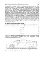
2. Propagation Impairments Effecting Satellite Communication Links
The use of satellite communication systems for modern broadband wireless services
involves propagation environments for radio signals different from that in conventional
terrestrial radio systems. The radio waves propagating between a satellite and an earth
station experience different kinds of propagation impairments: the effects of the ionosphere,
the troposphere and the local fading effects as shown in Fig. 1. The combined effect of these
7
Satellite Communications134
impairments on a satellite-earth link can cause random fluctuations in amplitude, phase,
angles of arrivals, de-polarization of electromagnetic waves and shadowing which result in
degradation of the signal quality and increase in the error rates of the communication links.


Fig. 1. The land-Mobile-Satellite Communication System

2.1 Ionospheric Effects
The effects of the ionosphere (an ionized section of the space extending from a height of 30
km to 1000 km) have adverse impact on the performance of earth-satellite radio propagation
links. These effects cause various impairments phenomena such as scintillation, polarization
rotation, refraction, group delays and dispersion etc, on the radio signals. The scintillation
and polarization rotation effects are of foremost concern for satellite communications.

Ionospheric scintillations are variations in the amplitude level, phase and angle of arrival of
the received radio waves. They are caused by the small irregularities in the refractive index
of the atmosphere owing to rapid variations in the local electron density. The main effect of
scintillation is fading that strongly depends on the irregularities or inhomogeneities of the

ionosphere (Ratcliffe, 1973; Blaunstein, 1995; Saunders & Zavala, 2007). Scintillation effects
are significant in two zones: at high altitudes (E and F layers of ionosphere) and the other is
±20º around the earth’s magnetic equator. The effects of scintillation decrease with increase
in operating frequency. It has been observed in various studies that at the operating
frequency of 4 GHz ionospheric scintillations can result in fades of several dBs and duration
between 1 to 10 seconds. The details about ionospheric scintillation can be found in
International Telecommunication Union Recommendations (ITU-R, 2009a).

The orthogonal polarization (linear or circular) is used in satellite communication systems to
increase the spectral efficiency without increasing the bandwidth requirements. This
technique, however, has limitations due to depolarization of electromagnetic waves
propagating through the atmosphere. When linearly polarized waves pass through the
ionosphere, the free electrons present in the ionosphere due to ionization interact with these
waves under the influence of the earth’s magnetic field in a similar way as the magnetic
field of a motor acts on a current carrying conductor. This results in rotation of the plane of
polarization of electromagnetic waves, recognized as Faraday rotation. The magnitude of
Faraday rotation is proportional to the length of the path through the ionosphere, the
geomagnetic field strength and the electron density, and inversely proportional to the
square of the operating frequency. The polarization rotation is significant for small
percentages of time at frequencies 1 GHz or less. The effect of Faraday rotation is much
lower at higher frequencies even in the regions of strong ionospheric impairments and low
elevation angles, e.g., at frequency of 10 GHz, Faraday rotation remains below 1º and can be
ignored (ITU, 2002). Cross-polarization can also be caused by the antenna systems at each
side of the link. The effects of depolarization are investigated by two methods: cross-
polarization discrimination (XPD) and polarization isolation. The details can be found in
(Roddy, 2006; Saunders & Zavala, 2007).

2.2 Tropospheric Effects
The troposphere is the non-ionized lower portion of the earth’s atmosphere covering
altitudes from the ground surface up to a height of about 15 km of the atmosphere. The

impairments of this region on radio propagations include hydrometeors, e.g., clouds, rain,
snow, fog as well as moisture in atmosphere, gradient of temperature and sporadic
structures of wind streams both in horizontal and vertical directions. The effects imparted
by these impairments on radio signals are rain attenuation, depolarization, scintillation,
refraction, absorption, etc. The radio waves are degraded by these effects to varying degrees
as a function of geographic location, frequency and elevation angle with specific
characteristics. The tropospheric effects in LMS communication links become significant
when the operating frequency is greater than 1 GHz.

One of the major causes of attenuation for LMS communication links operating at frequency
bands greater than 10 GHz (e.g., Ku-Band) is rain on the transmission paths in tropospheric
region. The rain attenuation in the received signal amplitude is due to absorption and
scattering of the radio waves energy by raindrops. The attenuation is measured as a
function of rainfall rate and increases with increase in the operating frequency, rainfall rate
and low elevation angles (Ippolito, 2008). The rainfall rate is the rate at which rain would
accrue in a rain gauge placed in a specific region on the ground (e.g., at base station). The
procedure to calculate attenuation statistics due to rainfall along a satellite-earth link for
frequencies up to 30 GHz consists of estimating the attenuation that exceeds 0.001% of the
time from the rainfall rate that exceeds at the same percentage of time and has been detailed
in ITU-R recommendations (ITU-R, 2007).

The LMS channel utilization can be augmented without increasing the transmission
bandwidth by the use of orthogonally polarized transmissions (linear or circular). The
polarization of radio waves can be altered by raindrops or ice particles in the transmission
path in such a way that power is transferred from the desired component to the undesired
component, resulting in interference between two orthogonally polarized channels. The
shape of small raindrops is spherical due to surface tension forces, but large raindrops adopt
shape of spheroids (having flat base) produced by aerodynamic forces acting in upward
Characterisation and Channel Modelling for Satellite Communication Systems 135
impairments on a satellite-earth link can cause random fluctuations in amplitude, phase,

angles of arrivals, de-polarization of electromagnetic waves and shadowing which result in
degradation of the signal quality and increase in the error rates of the communication links.


Fig. 1. The land-Mobile-Satellite Communication System

2.1 Ionospheric Effects
The effects of the ionosphere (an ionized section of the space extending from a height of 30
km to 1000 km) have adverse impact on the performance of earth-satellite radio propagation
links. These effects cause various impairments phenomena such as scintillation, polarization
rotation, refraction, group delays and dispersion etc, on the radio signals. The scintillation
and polarization rotation effects are of foremost concern for satellite communications.

Ionospheric scintillations are variations in the amplitude level, phase and angle of arrival of
the received radio waves. They are caused by the small irregularities in the refractive index
of the atmosphere owing to rapid variations in the local electron density. The main effect of
scintillation is fading that strongly depends on the irregularities or inhomogeneities of the
ionosphere (Ratcliffe, 1973; Blaunstein, 1995; Saunders & Zavala, 2007). Scintillation effects
are significant in two zones: at high altitudes (E and F layers of ionosphere) and the other is
±20º around the earth’s magnetic equator. The effects of scintillation decrease with increase
in operating frequency. It has been observed in various studies that at the operating
frequency of 4 GHz ionospheric scintillations can result in fades of several dBs and duration
between 1 to 10 seconds. The details about ionospheric scintillation can be found in
International Telecommunication Union Recommendations (ITU-R, 2009a).

The orthogonal polarization (linear or circular) is used in satellite communication systems to
increase the spectral efficiency without increasing the bandwidth requirements. This
technique, however, has limitations due to depolarization of electromagnetic waves
propagating through the atmosphere. When linearly polarized waves pass through the
ionosphere, the free electrons present in the ionosphere due to ionization interact with these

waves under the influence of the earth’s magnetic field in a similar way as the magnetic
field of a motor acts on a current carrying conductor. This results in rotation of the plane of
polarization of electromagnetic waves, recognized as Faraday rotation. The magnitude of
Faraday rotation is proportional to the length of the path through the ionosphere, the
geomagnetic field strength and the electron density, and inversely proportional to the
square of the operating frequency. The polarization rotation is significant for small
percentages of time at frequencies 1 GHz or less. The effect of Faraday rotation is much
lower at higher frequencies even in the regions of strong ionospheric impairments and low
elevation angles, e.g., at frequency of 10 GHz, Faraday rotation remains below 1º and can be
ignored (ITU, 2002). Cross-polarization can also be caused by the antenna systems at each
side of the link. The effects of depolarization are investigated by two methods: cross-
polarization discrimination (XPD) and polarization isolation. The details can be found in
(Roddy, 2006; Saunders & Zavala, 2007).

2.2 Tropospheric Effects
The troposphere is the non-ionized lower portion of the earth’s atmosphere covering
altitudes from the ground surface up to a height of about 15 km of the atmosphere. The
impairments of this region on radio propagations include hydrometeors, e.g., clouds, rain,
snow, fog as well as moisture in atmosphere, gradient of temperature and sporadic
structures of wind streams both in horizontal and vertical directions. The effects imparted
by these impairments on radio signals are rain attenuation, depolarization, scintillation,
refraction, absorption, etc. The radio waves are degraded by these effects to varying degrees
as a function of geographic location, frequency and elevation angle with specific
characteristics. The tropospheric effects in LMS communication links become significant
when the operating frequency is greater than 1 GHz.

One of the major causes of attenuation for LMS communication links operating at frequency
bands greater than 10 GHz (e.g., Ku-Band) is rain on the transmission paths in tropospheric
region. The rain attenuation in the received signal amplitude is due to absorption and
scattering of the radio waves energy by raindrops. The attenuation is measured as a

function of rainfall rate and increases with increase in the operating frequency, rainfall rate
and low elevation angles (Ippolito, 2008). The rainfall rate is the rate at which rain would
accrue in a rain gauge placed in a specific region on the ground (e.g., at base station). The
procedure to calculate attenuation statistics due to rainfall along a satellite-earth link for
frequencies up to 30 GHz consists of estimating the attenuation that exceeds 0.001% of the
time from the rainfall rate that exceeds at the same percentage of time and has been detailed
in ITU-R recommendations (ITU-R, 2007).

The LMS channel utilization can be augmented without increasing the transmission
bandwidth by the use of orthogonally polarized transmissions (linear or circular). The
polarization of radio waves can be altered by raindrops or ice particles in the transmission
path in such a way that power is transferred from the desired component to the undesired
component, resulting in interference between two orthogonally polarized channels. The
shape of small raindrops is spherical due to surface tension forces, but large raindrops adopt
shape of spheroids (having flat base) produced by aerodynamic forces acting in upward
Satellite Communications136
direction on the raindrops. When a linearly polarized wave passes through raindrops of
non-spherical structure, the vertical component of radio wave parallel to minor axis of
raindrops experiences less attenuation than that the horizontal component. As a result, there
will be a difference in the amount of attenuation and phase shift experienced by each of the
wave components. These differences cause depolarization of radio waves in the LMS links
and are illustrated as differential attenuation and differential phase shift. Rain and ice
depolarization have significant impacts on satellite-earth radio links for frequency bands
above 12 GHz, especially for systems employing independent dual orthogonally polarized
channels in the same frequency band in order to increase the capacity. The method of
predicting the long-term depolarization statistics has been described in ITU-R
recommendations (ITU-R, 2007).

A radio wave propagating through satellite-earth communication link will experience
reduction in the received signal’s amplitude level due to attenuation by different gases

(oxygen, nitrogen, hydrogen, etc.) present in the atmosphere. The amount of fading due to
gases is characterized mainly by altitude above sea level, frequency, temperature, pressure
and water vapour concentration. The principal cause of signal attenuation due to
atmospheric gases is molecular absorption. The absorption of radio waves occurs due to
conversion of radio wave energy to thermal energy at some specific resonant frequency of
the particles (quantum-level change in the rotational energy of the gas molecules). Among
different gases only water vapours and oxygen have resonant frequencies in the band of
interest up to 100 GHz. The attenuation due to atmospheric gases is normally neglected at
frequency bands below 10 GHz. A procedure to find out the effects of gaseous attenuation
on LMS links has been discussed in ITU-R recommendations (ITU-R, 2009b).

Scintillations (rapid variations in the received signal level, phase and angle-of-arrival) occur
due to inhomogeneities in the refractive index of atmosphere and influence low margin
satellite systems. The tropospheric scintillations can be severe at low elevation angles and
frequency bands above 10 GHz. Multipath effects can be observed for small percentages of
time at very low elevation angles (≤ 4º) due to large scale scintillation effects resulting in
signal attenuation greater than 10 dB.

2.3 Local Effects
In addition to the ionospheric and the tropospheric attenuation effects, radio waves suffer
from energy loss due to complex and varying propagation environments on the terrain. An
earth station is surrounded by different obstacles (buildings, trees, vegetation etc) of varying
heights, dimensions and of different densities. These obstructions cause different multipath
propagation phenomena: diffraction due to bending of the signal around edges of buildings,
dispersion or scattering by the interaction with objects of uneven shapes or surfaces,
specular reflection of the waves from objects with dimensions greater than the wavelength
of the radio waves, absorption through foliage etc. In addition, the movement of mobile
station on earth over short distances on the order of few wavelengths or over short time
durations on the order of few seconds results in rapid changes in the signal strength due to
changes in phases (Doppler Effect). All these effects result in loss of the signal energy and

degrade the performance and reliability of LMS communications links. A detailed
discussion about local effects on LMS communication links can be found in (Goldhirsh &
Vogel, 1998; Blaunstein & Christodoulou, 2007).

3. Probability Distribution Functions for Different Types of Fading
The performance of satellite-earth communication links depends on the operating
frequency, geographical location, climate, elevation angle to the satellite etc. The link
reliability of a satellite-based communication system decreases with the increase in
operating frequency and at low elevation angles. In addition, the random and unpredictable
nature of propagation environments increases complexity and uncertainty in the
characterization of transmission impairments on the LMS communication links. Therefore, it
is suitable to describe these phenomena in stochastic manner in order to assess the
performance of LMS communication systems over fading channels. Various precise and
elegant statistical distributions exist in the literature that can be used to characterize fading
effects in different propagation environments (Simon & Alouini, 2000; Corraza, 2007). In
general signal fading is decomposed as large scale path loss, a medium slowly varying
component following lognormal distribution and small scale fading in terms of Rayleigh or
Rice distributions depending on the existence of the LOS path between the transmitter and
the receiver. In this section, we give a brief overview of standard statistical distributions
used to model different fading effects on the LMS communication links.

3.1 Rayleigh Distribution
In case of heavily built-up areas (Urban Environments) the transmitted signal arrives at the
receiver through different multipath propagation mechanisms (section 2.3). The resultant
signal at the receiver is taken as the summation of diffuse multipath components
characterized by time-varying attenuations, different delays and phase shifts. When the
number of paths increase the sum approaches to complex Gaussian random variable having
independent real and imaginary parts with zero mean and equal variance. The amplitude of
the composite signal follows Rayleigh distribution and the phases of individual components
are uniformly distributed in the interval 0 to


2 . The received signal (real part) can be
written as:

 



n
i
iciRay
tttaR
1
)(cos)(

ni , ,2,1,0

(1)
where
)(ta
i
is the amplitude, )(t
i

is the phase of the
th
i multipath component and
c



represents the angular frequency of the carrier. The corresponding probability density
function (pdf) of the received signal’s envelope is expressed in the following mathematical
form:

)
2
exp()(
2
2
2


r
r
rP
Ray


0r (2)

where

denotes the standard deviation and ‘r ‘ represents envelop of the received signal.

Characterisation and Channel Modelling for Satellite Communication Systems 137
direction on the raindrops. When a linearly polarized wave passes through raindrops of
non-spherical structure, the vertical component of radio wave parallel to minor axis of
raindrops experiences less attenuation than that the horizontal component. As a result, there
will be a difference in the amount of attenuation and phase shift experienced by each of the
wave components. These differences cause depolarization of radio waves in the LMS links

and are illustrated as differential attenuation and differential phase shift. Rain and ice
depolarization have significant impacts on satellite-earth radio links for frequency bands
above 12 GHz, especially for systems employing independent dual orthogonally polarized
channels in the same frequency band in order to increase the capacity. The method of
predicting the long-term depolarization statistics has been described in ITU-R
recommendations (ITU-R, 2007).

A radio wave propagating through satellite-earth communication link will experience
reduction in the received signal’s amplitude level due to attenuation by different gases
(oxygen, nitrogen, hydrogen, etc.) present in the atmosphere. The amount of fading due to
gases is characterized mainly by altitude above sea level, frequency, temperature, pressure
and water vapour concentration. The principal cause of signal attenuation due to
atmospheric gases is molecular absorption. The absorption of radio waves occurs due to
conversion of radio wave energy to thermal energy at some specific resonant frequency of
the particles (quantum-level change in the rotational energy of the gas molecules). Among
different gases only water vapours and oxygen have resonant frequencies in the band of
interest up to 100 GHz. The attenuation due to atmospheric gases is normally neglected at
frequency bands below 10 GHz. A procedure to find out the effects of gaseous attenuation
on LMS links has been discussed in ITU-R recommendations (ITU-R, 2009b).

Scintillations (rapid variations in the received signal level, phase and angle-of-arrival) occur
due to inhomogeneities in the refractive index of atmosphere and influence low margin
satellite systems. The tropospheric scintillations can be severe at low elevation angles and
frequency bands above 10 GHz. Multipath effects can be observed for small percentages of
time at very low elevation angles (≤ 4º) due to large scale scintillation effects resulting in
signal attenuation greater than 10 dB.

2.3 Local Effects
In addition to the ionospheric and the tropospheric attenuation effects, radio waves suffer
from energy loss due to complex and varying propagation environments on the terrain. An

earth station is surrounded by different obstacles (buildings, trees, vegetation etc) of varying
heights, dimensions and of different densities. These obstructions cause different multipath
propagation phenomena: diffraction due to bending of the signal around edges of buildings,
dispersion or scattering by the interaction with objects of uneven shapes or surfaces,
specular reflection of the waves from objects with dimensions greater than the wavelength
of the radio waves, absorption through foliage etc. In addition, the movement of mobile
station on earth over short distances on the order of few wavelengths or over short time
durations on the order of few seconds results in rapid changes in the signal strength due to
changes in phases (Doppler Effect). All these effects result in loss of the signal energy and
degrade the performance and reliability of LMS communications links. A detailed
discussion about local effects on LMS communication links can be found in (Goldhirsh &
Vogel, 1998; Blaunstein & Christodoulou, 2007).

3. Probability Distribution Functions for Different Types of Fading
The performance of satellite-earth communication links depends on the operating
frequency, geographical location, climate, elevation angle to the satellite etc. The link
reliability of a satellite-based communication system decreases with the increase in
operating frequency and at low elevation angles. In addition, the random and unpredictable
nature of propagation environments increases complexity and uncertainty in the
characterization of transmission impairments on the LMS communication links. Therefore, it
is suitable to describe these phenomena in stochastic manner in order to assess the
performance of LMS communication systems over fading channels. Various precise and
elegant statistical distributions exist in the literature that can be used to characterize fading
effects in different propagation environments (Simon & Alouini, 2000; Corraza, 2007). In
general signal fading is decomposed as large scale path loss, a medium slowly varying
component following lognormal distribution and small scale fading in terms of Rayleigh or
Rice distributions depending on the existence of the LOS path between the transmitter and
the receiver. In this section, we give a brief overview of standard statistical distributions
used to model different fading effects on the LMS communication links.


3.1 Rayleigh Distribution
In case of heavily built-up areas (Urban Environments) the transmitted signal arrives at the
receiver through different multipath propagation mechanisms (section 2.3). The resultant
signal at the receiver is taken as the summation of diffuse multipath components
characterized by time-varying attenuations, different delays and phase shifts. When the
number of paths increase the sum approaches to complex Gaussian random variable having
independent real and imaginary parts with zero mean and equal variance. The amplitude of
the composite signal follows Rayleigh distribution and the phases of individual components
are uniformly distributed in the interval 0 to

2 . The received signal (real part) can be
written as:

 



n
i
iciRay
tttaR
1
)(cos)(

ni , ,2,1,0

(1)
where
)(ta
i

is the amplitude, )(t
i

is the phase of the
th
i multipath component and
c


represents the angular frequency of the carrier. The corresponding probability density
function (pdf) of the received signal’s envelope is expressed in the following mathematical
form:

)
2
exp()(
2
2
2


r
r
rP
Ray


0r (2)

where


denotes the standard deviation and ‘r ‘ represents envelop of the received signal.

Satellite Communications138
3.2 Rician Distribution
In propagation scenarios when a LOS component is present between the transmitter and the
receiver, the signal arriving at the receiver is expressed as the sum of one dominant vector
and large number of independently fading uncorrelated multipath components with
amplitudes of the order of magnitude and phases uniformly distributed in the interval
(0,2

). The received signal is characterized by Rice distribution and is given as follows:


 



n
i
iciRice
tttaCR
1
)(cos)(

ni , ,2,1,0

(3)
where constant ‘C’ represents the magnitude of the LOS signal between the transmitter and
the receiver. Other parameters are the same as described for Rayleigh distribution. The pdf

of the envelope of the received signal is illustrated in the following mathematical form:






2
2
22
0
2
2
exp)(



rC
Cr
Rice
I
r
rP









(4)

where
0
I represents the modified Bessel function of first kind and zero order, and
2
2
C
is
the mean power of the LOS component. If there is no direct path between the transmitter
and the receiver (i.e., C = 0) the above equation reduces to Rayleigh distribution. The ratio of
the average specular power (direct path) to the average fading power (multipath) over
specular paths is known as Rician factor (
2
2
2

a
) and is expressed in dBs.

3.3 Log-Normal Distribution
In addition to signal power loss due to hindrance of objects of large dimensions (buildings,
hills, etc), vegetation and foliage is another significant factor that cause scattering and
absorption of radio waves by trees with irregular pattern of branches and leaves with
different densities. As a result the power of the received signal varies about the mean power
predicted by the path loss. This type of variation in the received signal power is called
shadowing and is usually formulated as log-normally distributed over the ensemble of
typical locals. Shadowing creates holes in coverage areas and results in poor coverage and
poor carrier-to-interference ratio (CIR) in different places. The pdf of the received signal’s

envelope affected by shadowing follows lognormal distribution that can be written in the
following mathematical form:




















2
2
log
2
)(ln
2
1
exp

2
1
)(



r
r
rP
normal
0r (5)

where

and

are mean and standard deviation of the shadowed component of the
received signal, respectively.

3.4 Nakagami Distribution
As discussed in (Saunders & Zavala, 2007), the random fluctuations in the radio signal
propagating through the LMS communication channels can be categorized into two types of
fading: multipath fading and shadowing. The composite shadow fading (line-of-sight and
multiplicative shadowing) can be modelled by lognormal distribution. The application of
lognormal distribution to characterize shadowing effects results in complicated expressions
for the first and second order statistics and also the performance evaluation of
communication systems such as interference analysis and bit error rates become difficult.
An alternative to lognormal distribution is Nakagami distribution which can produce
simple statistical models with the same performance. The pdf of the received signal
envelope following Nakagami distribution is given by,





















2
2
12
2
2
exp
2
)(
2
)(


mr
r
m
m
rP
m
m
r
0r (6)

where (.) represents the Gamma function, )(2
22
rE

is the average power of the LOS
component and
2
1
m is the Nakagami-m parameter which varies between
2
1
to  . When
m increases the number of Gaussian random variables contributions increases and the
probability of deep fades in the corresponding pdf function decreases. Non-zero finite small
and large values of m correspond to urban and open areas, respectively. The intermediate
values of
m correspond to rural and suburban areas.

3.5 Suzuki Distribution

The Suzuki process is characterized as the product of Rayleigh distributed process and
lognormal process (Pätzold et al., 1998). Consider a Rayleigh distributed random variable

with pdf )(rP

and another random variable

following lognormal distribution with
pdf
)(rP

. Let

be a random variable defined by the product of these two independent
variables (



. ). The pdf
)(rP

of

can be written as follows:

































2
2
1
2

0
1
2
0
ln
exp.exp.
2
)(
2
0
2
2
3







mr
r
rP
z
r
r
0r (7)
This type of distribution can be used to represent propagation scenarios when LOS
component is absent in the received signal.


4. Statistical Channel Models for Land-Mobile-Satellite Communications
The influence of radio channel is a critical issue for the design, real-time operation and
performance assessment of LMS communication systems providing voice, text and
multimedia services operating at radio frequencies ranging from 100 MHz to 100 GHz and
optical frequencies. Thus, a good and accurate understanding of radio propagation channel
Characterisation and Channel Modelling for Satellite Communication Systems 139
3.2 Rician Distribution
In propagation scenarios when a LOS component is present between the transmitter and the
receiver, the signal arriving at the receiver is expressed as the sum of one dominant vector
and large number of independently fading uncorrelated multipath components with
amplitudes of the order of magnitude and phases uniformly distributed in the interval
(0,2

). The received signal is characterized by Rice distribution and is given as follows:


 



n
i
iciRice
tttaCR
1
)(cos)(

ni , ,2,1,0

(3)

where constant ‘C’ represents the magnitude of the LOS signal between the transmitter and
the receiver. Other parameters are the same as described for Rayleigh distribution. The pdf
of the envelope of the received signal is illustrated in the following mathematical form:






2
2
22
0
2
2
exp)(



rC
Cr
Rice
I
r
rP









(4)

where
0
I represents the modified Bessel function of first kind and zero order, and
2
2
C
is
the mean power of the LOS component. If there is no direct path between the transmitter
and the receiver (i.e., C = 0) the above equation reduces to Rayleigh distribution. The ratio of
the average specular power (direct path) to the average fading power (multipath) over
specular paths is known as Rician factor (
2
2
2

a
) and is expressed in dBs.

3.3 Log-Normal Distribution
In addition to signal power loss due to hindrance of objects of large dimensions (buildings,
hills, etc), vegetation and foliage is another significant factor that cause scattering and
absorption of radio waves by trees with irregular pattern of branches and leaves with
different densities. As a result the power of the received signal varies about the mean power
predicted by the path loss. This type of variation in the received signal power is called
shadowing and is usually formulated as log-normally distributed over the ensemble of

typical locals. Shadowing creates holes in coverage areas and results in poor coverage and
poor carrier-to-interference ratio (CIR) in different places. The pdf of the received signal’s
envelope affected by shadowing follows lognormal distribution that can be written in the
following mathematical form:




















2
2
log
2
)(ln
2

1
exp
2
1
)(



r
r
rP
normal
0r (5)

where

and

are mean and standard deviation of the shadowed component of the
received signal, respectively.

3.4 Nakagami Distribution
As discussed in (Saunders & Zavala, 2007), the random fluctuations in the radio signal
propagating through the LMS communication channels can be categorized into two types of
fading: multipath fading and shadowing. The composite shadow fading (line-of-sight and
multiplicative shadowing) can be modelled by lognormal distribution. The application of
lognormal distribution to characterize shadowing effects results in complicated expressions
for the first and second order statistics and also the performance evaluation of
communication systems such as interference analysis and bit error rates become difficult.
An alternative to lognormal distribution is Nakagami distribution which can produce

simple statistical models with the same performance. The pdf of the received signal
envelope following Nakagami distribution is given by,




















2
2
12
2
2
exp
2
)(

2
)(

mr
r
m
m
rP
m
m
r
0r (6)

where (.) represents the Gamma function, )(2
22
rE

is the average power of the LOS
component and
2
1
m is the Nakagami-m parameter which varies between
2
1
to  . When
m increases the number of Gaussian random variables contributions increases and the
probability of deep fades in the corresponding pdf function decreases. Non-zero finite small
and large values of m correspond to urban and open areas, respectively. The intermediate
values of
m correspond to rural and suburban areas.


3.5 Suzuki Distribution
The Suzuki process is characterized as the product of Rayleigh distributed process and
lognormal process (Pätzold et al., 1998). Consider a Rayleigh distributed random variable

with pdf )(rP

and another random variable

following lognormal distribution with
pdf
)(rP

. Let

be a random variable defined by the product of these two independent
variables (



. ). The pdf
)(rP

of

can be written as follows:

































2
2

1
2
0
1
2
0
ln
exp.exp.
2
)(
2
0
2
2
3







mr
r
rP
z
r
r
0r (7)
This type of distribution can be used to represent propagation scenarios when LOS

component is absent in the received signal.

4. Statistical Channel Models for Land-Mobile-Satellite Communications
The influence of radio channel is a critical issue for the design, real-time operation and
performance assessment of LMS communication systems providing voice, text and
multimedia services operating at radio frequencies ranging from 100 MHz to 100 GHz and
optical frequencies. Thus, a good and accurate understanding of radio propagation channel
Satellite Communications140
is of paramount significance in the design and implementation of satellite-based
communication systems.

The radio propagation channels can be developed using different approaches, e.g., physical
or deterministic techniques based on measured impulse responses and ray-tracing
algorithms which are complex and time consuming and statistical approach in which input
data and computational efforts are simple. The modelling of propagation effects on the LMS
communication links becomes highly complex and unpredictable owing to diverse nature of
radio propagation paths. Consequently statistical methods and analysis are generally the
most favourable approaches for the characterization of transmission impairments and
modelling of the LMS communication links.

The available statistical models for narrowband LMS channels can be characterized into two
categories: single state and multi-state models (Abdi et al., 2003). The single state models are
described by single statistical distributions and are valid for fixed satellite scenarios where
the channel statistics remain constant over the areas of interest. The multi-state or mixture
models are used to demonstrate non-stationary conditions where channel statistics vary
significantly over large areas for particular time intervals in nonuniform environments. In
this section, channel models developed for satellites based on statistical methods are
discussed.

4.1 Single-State Models

Loo Model: The Loo model is one of the most primitive statistical LMS channel model with
applications for rural environments specifically with shadowing due to roadside trees. In
this model the shadowing attenuation affecting the LOS signal due to foliage is
characterized by log-normal pdf and the diffuse multipath components are described by
Rayleigh pdf. The model illustrates the statistics of the channel in terms of probability
density and cumulative distribution functions under the assumption that foliage not only
attenuates but also scatters radio waves as well. The resulting complex signal envelope is
the sum of correlated lognormal and Rayleigh processes. The pdf of the received signal
envelope is given by (Loo, 1985; Loo & Butterworth, 1998).


 
 
















0

2
0
2
ln
2
1
brfor exp
brfor exp
)(
0
2
0
0
2
0
b
r
b
r
d
r
dr
rP


(8)

where µ and
0
d are the mean and standard deviation, respectively. The parameter

0
b denotes the average scattered power due to multipath effects. Note that if attenuation
due to shadowing (lognormal distribution) is kept constant then the pdf in (8) simply yields
in Rician distribution. This model has been verified experimentally by conducting
measurements in rural areas with elevation angles up to

30 (Loo et al., 1998).

Corraza-Vatalaro Model: In this model, a combination of Rice and lognormal distribution is
used to model effects of shadowing on both the LOS and diffuse components (Corazza &
Vatalaro, 1994) The model is suitable for non-geostationary satellite channels such as
medium-earth orbit (MEO) and low-earth orbit (LEO) channels and can be applied to
different environments (e.g., urban, suburban, rural) by simply adjusting the model
parameters. The pdf of the received signal envelop can be written as:


dSspSrprP
Sr



0
)(
)()()(
(9)

where )( Srp denotes conditional pdf following Rice distribution conditioned on
shadowing S (Corazza et al., 1994)





))1(2(.)1(exp)1(2)(
0
2
2
2
 KKIKKKSrP
S
r
S
r
S
r
0r (10)

where
K
is Rician factor (section 3.2) and
0
I is zero order modified Bessel function of first
kind. The pdf of lognormal of shadowing S, is given by:













2
ln
2
1
2
1
exp)(



h
S
Sh
S
SP 0S (11)

where
,20)10ln(h µ and
2
)(

h are mean and variance of the associated normal
variance, respectively. The received signal envelop can be interpreted as the product of two
independent processes (lognormal and Rice) with cumulative distribution function in the
following form (Corraza & Vatalaro, 1994):



 
 
))1(2,2(1)(
)(
)(
0
0
0 0
00



KKQEdrdSP
S
SP
rrPrP
S
r
S
S
r
r
r
S
r
(12)
where E(.) denotes the average with respect to S and Q is Marcum Q function.

The model is appropriate for different propagation conditions and has been verified using

experimental data with wide range of elevation angles as compared to Loo’s model.

Extended-Suzuki Model: A statistical channel model for terrestrial communications
characterized by Rayleigh and lognormal process is known as Suzuki model (Suzuki, 1977).
This model is suitable for modelling random variations of the signal in different types of
urban environments. An extension to this model, for frequency non-selective satellite
communication channels, is presented in (Pätzold et al., 1998) by considering that for most
of the time a LOS component is present in the received signal. The extended Suzuki process
is the product of Rice and lognormal probability distribution functions where inphase and
quadrature components of Rice process are allowed to be mutually correlated and the LOS
Characterisation and Channel Modelling for Satellite Communication Systems 141
is of paramount significance in the design and implementation of satellite-based
communication systems.

The radio propagation channels can be developed using different approaches, e.g., physical
or deterministic techniques based on measured impulse responses and ray-tracing
algorithms which are complex and time consuming and statistical approach in which input
data and computational efforts are simple. The modelling of propagation effects on the LMS
communication links becomes highly complex and unpredictable owing to diverse nature of
radio propagation paths. Consequently statistical methods and analysis are generally the
most favourable approaches for the characterization of transmission impairments and
modelling of the LMS communication links.

The available statistical models for narrowband LMS channels can be characterized into two
categories: single state and multi-state models (Abdi et al., 2003). The single state models are
described by single statistical distributions and are valid for fixed satellite scenarios where
the channel statistics remain constant over the areas of interest. The multi-state or mixture
models are used to demonstrate non-stationary conditions where channel statistics vary
significantly over large areas for particular time intervals in nonuniform environments. In
this section, channel models developed for satellites based on statistical methods are

discussed.

4.1 Single-State Models
Loo Model: The Loo model is one of the most primitive statistical LMS channel model with
applications for rural environments specifically with shadowing due to roadside trees. In
this model the shadowing attenuation affecting the LOS signal due to foliage is
characterized by log-normal pdf and the diffuse multipath components are described by
Rayleigh pdf. The model illustrates the statistics of the channel in terms of probability
density and cumulative distribution functions under the assumption that foliage not only
attenuates but also scatters radio waves as well. The resulting complex signal envelope is
the sum of correlated lognormal and Rayleigh processes. The pdf of the received signal
envelope is given by (Loo, 1985; Loo & Butterworth, 1998).


 
 

















0
2
0
2
ln
2
1
brfor exp
brfor exp
)(
0
2
0
0
2
0
b
r
b
r
d
r
dr
rP


(8)


where µ and
0
d are the mean and standard deviation, respectively. The parameter
0
b denotes the average scattered power due to multipath effects. Note that if attenuation
due to shadowing (lognormal distribution) is kept constant then the pdf in (8) simply yields
in Rician distribution. This model has been verified experimentally by conducting
measurements in rural areas with elevation angles up to

30 (Loo et al., 1998).

Corraza-Vatalaro Model: In this model, a combination of Rice and lognormal distribution is
used to model effects of shadowing on both the LOS and diffuse components (Corazza &
Vatalaro, 1994) The model is suitable for non-geostationary satellite channels such as
medium-earth orbit (MEO) and low-earth orbit (LEO) channels and can be applied to
different environments (e.g., urban, suburban, rural) by simply adjusting the model
parameters. The pdf of the received signal envelop can be written as:


dSspSrprP
Sr



0
)(
)()()(
(9)

where )( Srp denotes conditional pdf following Rice distribution conditioned on

shadowing S (Corazza et al., 1994)




))1(2(.)1(exp)1(2)(
0
2
2
2
 KKIKKKSrP
S
r
S
r
S
r
0r (10)

where
K
is Rician factor (section 3.2) and
0
I is zero order modified Bessel function of first
kind. The pdf of lognormal of shadowing S, is given by:













2
ln
2
1
2
1
exp)(



h
S
Sh
S
SP 0S (11)

where
,20)10ln(h µ and
2
)(

h are mean and variance of the associated normal
variance, respectively. The received signal envelop can be interpreted as the product of two

independent processes (lognormal and Rice) with cumulative distribution function in the
following form (Corraza & Vatalaro, 1994):


 
 
))1(2,2(1)(
)(
)(
0
0
0 0
00



KKQEdrdSP
S
SP
rrPrP
S
r
S
S
r
r
r
S
r
(12)

where E(.) denotes the average with respect to S and Q is Marcum Q function.

The model is appropriate for different propagation conditions and has been verified using
experimental data with wide range of elevation angles as compared to Loo’s model.

Extended-Suzuki Model: A statistical channel model for terrestrial communications
characterized by Rayleigh and lognormal process is known as Suzuki model (Suzuki, 1977).
This model is suitable for modelling random variations of the signal in different types of
urban environments. An extension to this model, for frequency non-selective satellite
communication channels, is presented in (Pätzold et al., 1998) by considering that for most
of the time a LOS component is present in the received signal. The extended Suzuki process
is the product of Rice and lognormal probability distribution functions where inphase and
quadrature components of Rice process are allowed to be mutually correlated and the LOS
Satellite Communications142
component is frequency shifted due to Doppler shift. The pdf of the extended Suzuki
process can be written as (Pätzold et al., 1998):


dyyPrP
y
r
y
),()(
1





(13)


where
),( yxP

denotes the joint pdf of the independent Rician and lognormal processes
)(t

and )(t

, and yrx  where y is variable of integration. The pdfs of Rice and
lognormal processes can be used in (13) to obtain the following pdf:




)(exp).(.exp)(
22
)(ln
0
0
2
))((
1
2
2
00
22
3
0




my
y
rp
p
y
r
IrP
y
r


















0r (14)


where
0

is the mean value of random variable ,
x
m and µ are the mean and standard
deviation of random variable y and p denotes LOS component.

The model was verified experimentally with operating frequency of 870 MHz at an
elevation angle

15 in rural area with 35% trees coverage. Two scenarios were selected: a
lightly shadowed scenario and a heavily shadowed scenario with dense trees coverage. The
cumulative distribution functions of the measurement data were in good agreement with
those obtained from analytical extended Suzuki model.

Xie-Fang Model: This model (Xie & Fang, 2000), based on propagation scattering theory,
deals with the statistical modelling of propagation characteristics in LEO and MEO satellites
communication systems. In these satellites communication systems a mobile user or a
satellite can move during communication sessions and as a result the received signals may
fluctuate from time to time. The quality-of-service (QoS) degrades owing to random
fluctuations in the received signal level caused by different propagation impairments in the
LMS communication links (section 2). In order to efficiently design a satellite
communication system, these propagation effects need to be explored. This channel model
deals with the statistical characterization of such propagation channels.

In satellite communications operating at low elevation angles, the use of small antennas as
well as movement of the receiver or the transmitter introduces the probability of path
blockage and multipath scattering components which result in random fluctuations in the

received signal causing various fading phenomena. In this model fading is characterized as
two independent random processes: short-term (small scale) fading and long-term fading.
The long term fading is modelled by lognormal distribution and the small scale fading is
characterized by a more general form of Rician distribution. It is assumed, based on
scattering theory of electromagnetic waves, that the amplitudes and phases of the scattering
components which cause small scale fading due to superposition are correlated. The total
electric field is the sum of multipath signals arriving at the receiver (Beckman et al., 1987):




n
i
iitot
jAjEE
1
)exp()exp(

(15)
where n denotes the number of paths,
i
A and
i

represent the amplitude and phase of the
th
i path component, respectively. The pdf of the received signal envelope can be obtained as
follows (Xie & Fang, 2000):








d
SS
rSSrSrS
SS
SSrS
SS
r
rP
r






















2
0
21
22
2112
21
2
1
2
2
2
1
21
2
cos)(sin2cos2
exp
2
1
2
exp)(
(16)

and the pdf of the received signal power envelope is given by:









d
SS
WSSWSWS
SS
SSWS
SS
WP
p






















2
0
21
2
2112
21
2
2
2
12
21
2
cos)(sin2cos2
exp
2
1
2
exp
2
1
)(
(17)

where the parameters
,

1
S ,
2
S ,

and

denote the variances and means of the Gaussian
distributed real and imaginary parts of the received signal envelope ‘r’, respectively, and
‘W’ represents the power of the received signal.

This statistical LMS channel model concludes that the received signal from a satellite can be
expressed as the product of two independent random processes. The channel model is more
general in the sense that it can provide a good fit to experimental data and better
characterization of the propagation environments as compared to previously developed
statistical channel models.
Abdi Model: This channel model (Abdi et al., 2003) is convenient for performance
predictions of narrowband and wideband satellite communication systems. In this model
the amplitude of the shadowed LOS signal is characterized by Nakagami distribution
(section 3.4) and the multipath component of the total signal envelop is characterized by
Rayleigh distribution. The advantage of this model is that it results in mathematically
precise closed form expressions of the channel first order statistics such as signal envelop
pdf, moment generating functions of the instantaneous power and the second order channel
statistics such as average fade durations and level crossing rates (Abdi et al., 2003).
According to this model the low pass equivalent of the shadowed Rician signal’s complex
envelope can as:







)(exp)()(exp)()( tjtZtjtAtR




(18)

Characterisation and Channel Modelling for Satellite Communication Systems 143
component is frequency shifted due to Doppler shift. The pdf of the extended Suzuki
process can be written as (Pätzold et al., 1998):


dyyPrP
y
r
y
),()(
1





(13)

where
),( yxP


denotes the joint pdf of the independent Rician and lognormal processes
)(t

and )(t

, and yrx

where y is variable of integration. The pdfs of Rice and
lognormal processes can be used in (13) to obtain the following pdf:




)(exp).(.exp)(
22
)(ln
0
0
2
))((
1
2
2
00
22
3
0




my
y
rp
p
y
r
IrP
y
r


















0r (14)

where

0

is the mean value of random variable ,
x
m and µ are the mean and standard
deviation of random variable y and p denotes LOS component.

The model was verified experimentally with operating frequency of 870 MHz at an
elevation angle

15 in rural area with 35% trees coverage. Two scenarios were selected: a
lightly shadowed scenario and a heavily shadowed scenario with dense trees coverage. The
cumulative distribution functions of the measurement data were in good agreement with
those obtained from analytical extended Suzuki model.

Xie-Fang Model: This model (Xie & Fang, 2000), based on propagation scattering theory,
deals with the statistical modelling of propagation characteristics in LEO and MEO satellites
communication systems. In these satellites communication systems a mobile user or a
satellite can move during communication sessions and as a result the received signals may
fluctuate from time to time. The quality-of-service (QoS) degrades owing to random
fluctuations in the received signal level caused by different propagation impairments in the
LMS communication links (section 2). In order to efficiently design a satellite
communication system, these propagation effects need to be explored. This channel model
deals with the statistical characterization of such propagation channels.

In satellite communications operating at low elevation angles, the use of small antennas as
well as movement of the receiver or the transmitter introduces the probability of path
blockage and multipath scattering components which result in random fluctuations in the
received signal causing various fading phenomena. In this model fading is characterized as
two independent random processes: short-term (small scale) fading and long-term fading.

The long term fading is modelled by lognormal distribution and the small scale fading is
characterized by a more general form of Rician distribution. It is assumed, based on
scattering theory of electromagnetic waves, that the amplitudes and phases of the scattering
components which cause small scale fading due to superposition are correlated. The total
electric field is the sum of multipath signals arriving at the receiver (Beckman et al., 1987):




n
i
iitot
jAjEE
1
)exp()exp(

(15)
where n denotes the number of paths,
i
A and
i

represent the amplitude and phase of the
th
i path component, respectively. The pdf of the received signal envelope can be obtained as
follows (Xie & Fang, 2000):








d
SS
rSSrSrS
SS
SSrS
SS
r
rP
r






















2
0
21
22
2112
21
2
1
2
2
2
1
21
2
cos)(sin2cos2
exp
2
1
2
exp)(
(16)

and the pdf of the received signal power envelope is given by:









d
SS
WSSWSWS
SS
SSWS
SS
WP
p






















2
0
21
2
2112
21
2
2
2
12
21
2
cos)(sin2cos2
exp
2
1
2
exp
2
1
)(
(17)

where the parameters
,
1
S ,

2
S ,

and

denote the variances and means of the Gaussian
distributed real and imaginary parts of the received signal envelope ‘r’, respectively, and
‘W’ represents the power of the received signal.

This statistical LMS channel model concludes that the received signal from a satellite can be
expressed as the product of two independent random processes. The channel model is more
general in the sense that it can provide a good fit to experimental data and better
characterization of the propagation environments as compared to previously developed
statistical channel models.
Abdi Model: This channel model (Abdi et al., 2003) is convenient for performance
predictions of narrowband and wideband satellite communication systems. In this model
the amplitude of the shadowed LOS signal is characterized by Nakagami distribution
(section 3.4) and the multipath component of the total signal envelop is characterized by
Rayleigh distribution. The advantage of this model is that it results in mathematically
precise closed form expressions of the channel first order statistics such as signal envelop
pdf, moment generating functions of the instantaneous power and the second order channel
statistics such as average fade durations and level crossing rates (Abdi et al., 2003).
According to this model the low pass equivalent of the shadowed Rician signal’s complex
envelope can as:







)(exp)()(exp)()( tjtZtjtAtR


 (18)

Satellite Communications144
where )(tA and )(tZ are independent stationary random processes representing the
amplitudes of the scattered and LOS components, respectively. The independent stationary
random process,
)(t

, uniformly distributed over (0, 2

) denotes the phase of scattered
components and
)(t

is the deterministic phase of LOS component. The pdf of the received
signal envelop for the first order statistics of the model can be written as (Abdi et al., 2003):































)2(2
,1,
2
exp.
2
2
)(
00
2
11
0

2
00
0
mbb
r
mF
b
r
b
r
mb
mb
rP
m
r
0r (19)

where
0
2b is the average power of the multipath component,

is the average power of the
LOS component and
(.)
11
F is the confluent hypergeometric function.

The channel model’s first order and second order statistics compared with different
available data sets, demonstrate the appropriateness of the model in characterizing various
channel conditions over satellite communication links. This model illustrates similar

agreements with the experimental data as the Loo’s model and is suitable for the numerical
and analytical performance predictions of narrowband and wideband LMS communication
systems with different types of encoded/decoded modulations.

4.2 Multi-state Models
In the case of nonstationary conditions when terminals (either satellite or mobile terminal)
move in a large area of a nonuniform environment, the received signal statistics may change
significantly over the observation interval. Therefore, propagation characteristics of such
environments are appropriately characterized by the so-called multi-state models.

Markov models are very popular because they are computationally efficient, analytically
tractable with well established theory and have been successfully applied to characterize
fading channels, to evaluate capacity of fading channels and in the design of optimum error
correcting coding techniques (Tranter et al., 2003). Markov models are characterized in
terms of state probability and state probability transition matrices. In multi-state channel
models, each state is characterized by an underlying Markov process in terms of one of the
single state models discussed in the previous section.

Lutz Model: Lutz’s model (Lutz et al., 1991) is two-state (good state and bad state) statistical
model based on data obtained from measurement campaigns in different parts of Europe at
elevation angles between 13° to 43° and is appropriate for the characterization of radio wave
propagation in urban and suburban areas. The good state represents LOS condition in
which the received signal follows Rician distribution with Rice factor K which depends on
the operating frequency and the satellite elevation angle. The bad state models the signal
amplitude to be Rayleigh distributed with mean power
2
0

S which fluctuates with time.
Another important parameter of this model is time share of shadowing ‘A’. Therefore, pdf of

the received signal power can be written as follows (Lutz et al., 1991):




0
000
)()()().1()( dSSpSSpASpASp
LNRayRice
(20)
The values of the parameters A, K, means, variances and the associated probabilities have
been derived from measured data for different satellite elevations, antennas and
environments using curve fitting procedures. The details can be found in (Lutz et al., 1991).
Transitions between two states are described by first order Markov chain where transition
from one state to the next depends only on the current state. For two-state Lutz’ model, the
probabilities
ij
P
( bgji ,,

) represent transitions from sate i to state j according to good or
bad state as shown in Fig. 2.

Fig. 2. Lutz’s Two-state LMS channel model.

The transition probabilities can be determined in terms of the average distances
g
D
and
b

D
in meters over which the system remains in the good and bad states, respectively.


g
gb
D
vR
P 

b
bg
D
vR
P 
(21)

where v is the mobile speed in meters per second, R is the transmission data rate in bits per
second. As the sum of probabilities in any state is equal to unity, thus
gbgg
PP 1
and
.1
bgbb
PP 
The time share of shadowing can be obtained as:


gb
b

DD
D
A


(22)
The parameter A in this model is independent of data rate and mobile speed. For different
channel models, the time share of shadowing is obtained according to available propagation
conditions and parameters. For example in (Saunders & Evans, 1996) time share of
shadowing is calculated by considering buildings height distributions and street width etc.

Three-State Model: This statistical channel model (Karasawa et al., 1997), based on three
states, namely clear or LOS state, the shadowing state and the blocked state, provides the
analysis of availability improvement in non-geostationary LMS communication systems.
The clear state is characterized by Rice distribution, the shadowing state is described by
Characterisation and Channel Modelling for Satellite Communication Systems 145
where )(tA and )(tZ are independent stationary random processes representing the
amplitudes of the scattered and LOS components, respectively. The independent stationary
random process,
)(t

, uniformly distributed over (0, 2

) denotes the phase of scattered
components and
)(t

is the deterministic phase of LOS component. The pdf of the received
signal envelop for the first order statistics of the model can be written as (Abdi et al., 2003):































)2(2

,1,
2
exp.
2
2
)(
00
2
11
0
2
00
0
mbb
r
mF
b
r
b
r
mb
mb
rP
m
r
0r (19)

where
0
2b is the average power of the multipath component,


is the average power of the
LOS component and
(.)
11
F is the confluent hypergeometric function.

The channel model’s first order and second order statistics compared with different
available data sets, demonstrate the appropriateness of the model in characterizing various
channel conditions over satellite communication links. This model illustrates similar
agreements with the experimental data as the Loo’s model and is suitable for the numerical
and analytical performance predictions of narrowband and wideband LMS communication
systems with different types of encoded/decoded modulations.

4.2 Multi-state Models
In the case of nonstationary conditions when terminals (either satellite or mobile terminal)
move in a large area of a nonuniform environment, the received signal statistics may change
significantly over the observation interval. Therefore, propagation characteristics of such
environments are appropriately characterized by the so-called multi-state models.

Markov models are very popular because they are computationally efficient, analytically
tractable with well established theory and have been successfully applied to characterize
fading channels, to evaluate capacity of fading channels and in the design of optimum error
correcting coding techniques (Tranter et al., 2003). Markov models are characterized in
terms of state probability and state probability transition matrices. In multi-state channel
models, each state is characterized by an underlying Markov process in terms of one of the
single state models discussed in the previous section.

Lutz Model: Lutz’s model (Lutz et al., 1991) is two-state (good state and bad state) statistical
model based on data obtained from measurement campaigns in different parts of Europe at

elevation angles between 13° to 43° and is appropriate for the characterization of radio wave
propagation in urban and suburban areas. The good state represents LOS condition in
which the received signal follows Rician distribution with Rice factor K which depends on
the operating frequency and the satellite elevation angle. The bad state models the signal
amplitude to be Rayleigh distributed with mean power
2
0

S which fluctuates with time.
Another important parameter of this model is time share of shadowing ‘A’. Therefore, pdf of
the received signal power can be written as follows (Lutz et al., 1991):




0
000
)()()().1()( dSSpSSpASpASp
LNRayRice
(20)
The values of the parameters A, K, means, variances and the associated probabilities have
been derived from measured data for different satellite elevations, antennas and
environments using curve fitting procedures. The details can be found in (Lutz et al., 1991).
Transitions between two states are described by first order Markov chain where transition
from one state to the next depends only on the current state. For two-state Lutz’ model, the
probabilities
ij
P
( bgji ,,  ) represent transitions from sate i to state j according to good or
bad state as shown in Fig. 2.


Fig. 2. Lutz’s Two-state LMS channel model.

The transition probabilities can be determined in terms of the average distances
g
D
and
b
D
in meters over which the system remains in the good and bad states, respectively.


g
gb
D
vR
P 

b
bg
D
vR
P 
(21)

where v is the mobile speed in meters per second, R is the transmission data rate in bits per
second. As the sum of probabilities in any state is equal to unity, thus
gbgg
PP 1
and

.1
bgbb
PP 
The time share of shadowing can be obtained as:


gb
b
DD
D
A


(22)
The parameter A in this model is independent of data rate and mobile speed. For different
channel models, the time share of shadowing is obtained according to available propagation
conditions and parameters. For example in (Saunders & Evans, 1996) time share of
shadowing is calculated by considering buildings height distributions and street width etc.

Three-State Model: This statistical channel model (Karasawa et al., 1997), based on three
states, namely clear or LOS state, the shadowing state and the blocked state, provides the
analysis of availability improvement in non-geostationary LMS communication systems.
The clear state is characterized by Rice distribution, the shadowing state is described by
Satellite Communications146
Loo’s pdf and the blocked state is illustrated by Rayleigh fading as shown in Fig. 3(a), where
1
a denotes the LOS component,
2
a represents shadowing effects caused by trees
and

3
a represents blockage (perfect shadowing). Similarly, multipath contributions in the
form of coherently reflected waves from the ground are denoted by
1
b and incoherently
scattered components from the land obstructions are represented by
2
b . The pdf of the
received signal envelop is weighted linear combination of these distributions:


(r)NP(r)LP(r)MP(r)P
RayleighLooRiceR

(23)
where M, L, and N are the time share of shadowing of Rice, Loo and Rayleigh distributions,
respectively. The distribution parameters for the model were found by means of the data
obtained from measurements using “INMARSAT” satellite and other available data sets.
The model was validated by comparing the theoretical cumulative distributions with those
obtained from measurement data. The state transitions characteristics of the model were
obtained using Markov model as shown in Fig. 3(b). The state occurrence probability
functions
,
A
P
B
P and
c
P (where 1
CBA

PPP ) can be computed as follows (Karasawa et
al., 1997):

aP
A
/)90(
2


(24)
where

is the elevation angle of satellite (

 9010

) and ‘a’ is a constant with values:










areassuburban for
4
1066.1

areasurban for
3
100.7
a








areassuburban for 4
areasurban for
4
C
C
B
P
P
P
(25)

In order to characterize the state duration statistics such as the average distances or time
spans during which a particular state tends to persist, a model capable of providing time-
variant features is essential. A Markov process suitable for this purpose is expressed as
three-state model as shown in Fig. 3(b) (Karasawa et al., 1997). In this model short-term
fluctuations in the received signal are represented by specific pdfs within the states and
long-term fading is described by the transitions between the states. This model is also
suitable for the performance assessment of satellite diversity.


A significant aspect of the LMS systems is that a single satellite is not adequate for
achieving the desired coverage reliability with a high signal quality. Thus, it is desirable that
different satellite constellations should be employed which can improve the system
availability and signal quality by means of satellite diversity. If a link with one of the
satellites is interrupted by shadowing, an alternative satellite should be available to help
reduce the outage probability. This channel model also provides analysis for the
improvement of the signal quality and service availability by means of satellite diversity
where at least two satellites in LEO/MEO orbit, illuminate the coverage area simultaneously
in urban and suburban environments.
1
a
2
a
3
a
1
b
2
b
AA
P
BB
P
CC
P
A
C
P
CA

P
BC
P
CB
P
AB
P
BA
P

(a) (b)
Fig. 3. Three-sate LMS channel model (a) Propagation impairments (b) Markov model.

Five-State Model: This channel model is based on Markov modelling approach in which
two-state and three-state models are extended to five-state model under different time share
of shadowing (Ming et al., 2008). The model is basically a composition of Gilbert-Elliot
channel model and the three-state Markov channel model in which shadowing effects are
split into three states: ‘good’ state represents low shadowing, ‘not good not bad’ state
characterizes moderate shadowing and ‘bad state’ describes heavy or complete shadowing
as shown in Fig. 4 (Ming et al., 2008). The ‘good’ state has two sub-states: clear LOS without
shadowing and LOS state with low shadowing. Similarly, the ‘bad’ state has two sub-states:
heavily shadowed areas or completely shadowed or blocked areas. A state transition can
occur when the receiver is in low or high shadowing areas for a period of time. The
transitions can take place from low and high shadowing conditions to moderate shadowing
conditions but cannot occur directly between low and high shadowing environments.

For different shadowing effects, the statistical signal level characteristics in terms of the pdf
are described as: low shadowing follows Rice distribution, moderate shadowing is
represented by Loo’s pdf and high shadowing conditions are described by Rayleigh-
lognormal distribution. The pdf of the received signal power is a weighted linear

combination of these distributions:


)()()()()()(
2_51_432211
sPXsPXsPXsPXsPXsP
LRayLRayLooRiceRice

(26)
where
i
X )5, ,1( i are time share of shadowing of the states
i
S )5, ,1(

i , respectively.

The state probability and state transition probability matrices are determined using the time
series of the measured data. The channel model has been validated using available
measured data sets and different statistical parameters are obtained using curve fitting
procedures. The channel statistics like the cumulative distribution function, the level
crossing rate, the average fade duration, and the bit error rate are computed which show a
Characterisation and Channel Modelling for Satellite Communication Systems 147
Loo’s pdf and the blocked state is illustrated by Rayleigh fading as shown in Fig. 3(a), where
1
a denotes the LOS component,
2
a represents shadowing effects caused by trees
and
3

a represents blockage (perfect shadowing). Similarly, multipath contributions in the
form of coherently reflected waves from the ground are denoted by
1
b and incoherently
scattered components from the land obstructions are represented by
2
b . The pdf of the
received signal envelop is weighted linear combination of these distributions:


(r)NP(r)LP(r)MP(r)P
RayleighLooRiceR

(23)
where M, L, and N are the time share of shadowing of Rice, Loo and Rayleigh distributions,
respectively. The distribution parameters for the model were found by means of the data
obtained from measurements using “INMARSAT” satellite and other available data sets.
The model was validated by comparing the theoretical cumulative distributions with those
obtained from measurement data. The state transitions characteristics of the model were
obtained using Markov model as shown in Fig. 3(b). The state occurrence probability
functions
,
A
P
B
P and
c
P (where 1




CBA
PPP ) can be computed as follows (Karasawa et
al., 1997):

aP
A
/)90(
2


(24)
where

is the elevation angle of satellite (

 9010

) and ‘a’ is a constant with values:










areassuburban for

4
1066.1
areasurban for
3
100.7
a








areassuburban for 4
areasurban for
4
C
C
B
P
P
P
(25)

In order to characterize the state duration statistics such as the average distances or time
spans during which a particular state tends to persist, a model capable of providing time-
variant features is essential. A Markov process suitable for this purpose is expressed as
three-state model as shown in Fig. 3(b) (Karasawa et al., 1997). In this model short-term
fluctuations in the received signal are represented by specific pdfs within the states and

long-term fading is described by the transitions between the states. This model is also
suitable for the performance assessment of satellite diversity.

A significant aspect of the LMS systems is that a single satellite is not adequate for
achieving the desired coverage reliability with a high signal quality. Thus, it is desirable that
different satellite constellations should be employed which can improve the system
availability and signal quality by means of satellite diversity. If a link with one of the
satellites is interrupted by shadowing, an alternative satellite should be available to help
reduce the outage probability. This channel model also provides analysis for the
improvement of the signal quality and service availability by means of satellite diversity
where at least two satellites in LEO/MEO orbit, illuminate the coverage area simultaneously
in urban and suburban environments.
1
a
2
a
3
a
1
b
2
b
AA
P
BB
P
CC
P
A
C

P
CA
P
BC
P
CB
P
AB
P
BA
P

(a) (b)
Fig. 3. Three-sate LMS channel model (a) Propagation impairments (b) Markov model.

Five-State Model: This channel model is based on Markov modelling approach in which
two-state and three-state models are extended to five-state model under different time share
of shadowing (Ming et al., 2008). The model is basically a composition of Gilbert-Elliot
channel model and the three-state Markov channel model in which shadowing effects are
split into three states: ‘good’ state represents low shadowing, ‘not good not bad’ state
characterizes moderate shadowing and ‘bad state’ describes heavy or complete shadowing
as shown in Fig. 4 (Ming et al., 2008). The ‘good’ state has two sub-states: clear LOS without
shadowing and LOS state with low shadowing. Similarly, the ‘bad’ state has two sub-states:
heavily shadowed areas or completely shadowed or blocked areas. A state transition can
occur when the receiver is in low or high shadowing areas for a period of time. The
transitions can take place from low and high shadowing conditions to moderate shadowing
conditions but cannot occur directly between low and high shadowing environments.

For different shadowing effects, the statistical signal level characteristics in terms of the pdf
are described as: low shadowing follows Rice distribution, moderate shadowing is

represented by Loo’s pdf and high shadowing conditions are described by Rayleigh-
lognormal distribution. The pdf of the received signal power is a weighted linear
combination of these distributions:


)()()()()()(
2_51_432211
sPXsPXsPXsPXsPXsP
LRayLRayLooRiceRice

(26)
where
i
X )5, ,1( i are time share of shadowing of the states
i
S )5, ,1( i , respectively.

The state probability and state transition probability matrices are determined using the time
series of the measured data. The channel model has been validated using available
measured data sets and different statistical parameters are obtained using curve fitting
procedures. The channel statistics like the cumulative distribution function, the level
crossing rate, the average fade duration, and the bit error rate are computed which show a
Satellite Communications148
good agreement with the statistics of the data obtained from measurements. The channel
model is appropriate for urban and suburban areas.


Fig. 4. Five-state Markov channel model for LMS communications.

Modelling Frequency Selective LMS Channel: The LMS propagation channel effects

depend on the propagation impairments (section 2), geographical location, elevation angles
and operating frequency band. Extensive measurements are needed for the characterization
of LMS fading caused by different propagation impairments. When components of a signal
travelling through different paths arrive at the receiver with delays significantly larger as
compared to the bit or symbol duration, the signal will undergo significant amount of
distortion across the information bandwidth, it results in frequency selective fading or
wideband fading (e.g., in the case of broadband services or spread spectrum). The impulse
response of a wideband channel model (also known as tapped-delay line model) under
wide sense stationary uncorrelated scattering (WSSUS) assumption can be written as:


 
 
))()(2(exp)()(),(
,
1
ttfjtttath
iid
N
i
ii




(27)

where
),(ta
i

),(t
i

id
f
,
and
)(t
i

are the amplitude, delay, Doppler shift and phase of the
th
i
component of the received signal, respectively, and )(t

denotes the Dirac delta
function.

A tapped-delay line model that describes the wideband characteristics of LMS
communication link has been given in (Jahn, 2001). The parameters for this model are
extracted using extensive measurement data at L-band for different applications, scenarios
and environments. In order to adopt the channel for LMS communications, the channel
impulse response is divided into three components: the direct path, near echoes and far
echoes as shown in Fig. 5 (Jahn, 2001). The delays
i

), ,2,1( Ni

of the taps are taken with
respect to the delay of the direct path. The power of all taps is normalized to the power of

the direct path. The amplitude distributions of the echoes follow Rice or Rayleigh
distribution (section 3) depending on the presence of LOS or non-LOS situations,
respectively. The number
n
N of near echoes in the locality of the receiver follows Poisson
distribution with parameter

))()(.,.(
!



 eNfei
N
Poisson
N
and the corresponding delays
i

), ,2,1( Ni  characterizing near echoes follow exponential distribution with parameter
b
)}./()(.,.{
/
exp
befei
b
n
i
n
i




 The power of the taps decay exponentially. The far
echoes
,1
nf
NNN which are few in numbers are characterized by Poisson
distribution. The amplitude distributions of the far echoes are described by Rayleigh
distribution. The description of different regions of the wideband LMS channel impulse
response can be found in (Jahn, 2001). Another physical-statistical channel model that deals
with the frequency selectivity of LMS channels is found in (Parks et al., 1996). This model
consists of two cascaded processes. The first one deals with propagation effects from
satellite to earth and the second process illustrates the terrestrial propagation impairments.
c


max



n
N
f
N

Fig. 5. Wideband LMS channel impulse response with different regions.

5. Conclusions
This chapter provides an overview of propagation impairments on LMS communication

links, probability distributions describing these fading effects and channel models
developed using these probability distributions. Proper knowledge of propagation
impairments and channel models is necessary for the design and performance assessment of
advanced transceiver techniques employed to establish reliable communication links in LMS
communication systems. The main focus lies on highlighting which are the effects and the
relevant propagation models need to be considered for LMS communication links in order
to accurately estimate the propagation impairments. The performance of LMS
communication systems depend on different factors including operating frequency,
elevation angles, geographic location, climate etc. Different approaches can be used to find
the effects of these factors on LMS communication links such as physical-statistical channel
models which are more accurate but require long simulation times and are complex. On the
other hand statistical methods are simple and require less computational efforts. In addition,
due to diverse nature of propagation environments, it is appropriate to use stochastic
approaches for the performance assessment of LMS communication links.

Characterisation and Channel Modelling for Satellite Communication Systems 149
good agreement with the statistics of the data obtained from measurements. The channel
model is appropriate for urban and suburban areas.


Fig. 4. Five-state Markov channel model for LMS communications.

Modelling Frequency Selective LMS Channel: The LMS propagation channel effects
depend on the propagation impairments (section 2), geographical location, elevation angles
and operating frequency band. Extensive measurements are needed for the characterization
of LMS fading caused by different propagation impairments. When components of a signal
travelling through different paths arrive at the receiver with delays significantly larger as
compared to the bit or symbol duration, the signal will undergo significant amount of
distortion across the information bandwidth, it results in frequency selective fading or
wideband fading (e.g., in the case of broadband services or spread spectrum). The impulse

response of a wideband channel model (also known as tapped-delay line model) under
wide sense stationary uncorrelated scattering (WSSUS) assumption can be written as:


 
 
))()(2(exp)()(),(
,
1
ttfjtttath
iid
N
i
ii




(27)

where
),(ta
i
),(t
i

id
f
,
and

)(t
i

are the amplitude, delay, Doppler shift and phase of the
th
i
component of the received signal, respectively, and )(t

denotes the Dirac delta
function.

A tapped-delay line model that describes the wideband characteristics of LMS
communication link has been given in (Jahn, 2001). The parameters for this model are
extracted using extensive measurement data at L-band for different applications, scenarios
and environments. In order to adopt the channel for LMS communications, the channel
impulse response is divided into three components: the direct path, near echoes and far
echoes as shown in Fig. 5 (Jahn, 2001). The delays
i

), ,2,1( Ni

of the taps are taken with
respect to the delay of the direct path. The power of all taps is normalized to the power of
the direct path. The amplitude distributions of the echoes follow Rice or Rayleigh
distribution (section 3) depending on the presence of LOS or non-LOS situations,
respectively. The number
n
N of near echoes in the locality of the receiver follows Poisson
distribution with parameter


))()(.,.(
!



 eNfei
N
Poisson
N
and the corresponding delays
i

), ,2,1( Ni  characterizing near echoes follow exponential distribution with parameter
b
)}./()(.,.{
/
exp
befei
b
n
i
n
i



 The power of the taps decay exponentially. The far
echoes
,1
nf

NNN which are few in numbers are characterized by Poisson
distribution. The amplitude distributions of the far echoes are described by Rayleigh
distribution. The description of different regions of the wideband LMS channel impulse
response can be found in (Jahn, 2001). Another physical-statistical channel model that deals
with the frequency selectivity of LMS channels is found in (Parks et al., 1996). This model
consists of two cascaded processes. The first one deals with propagation effects from
satellite to earth and the second process illustrates the terrestrial propagation impairments.
c


max



n
N
f
N

Fig. 5. Wideband LMS channel impulse response with different regions.

5. Conclusions
This chapter provides an overview of propagation impairments on LMS communication
links, probability distributions describing these fading effects and channel models
developed using these probability distributions. Proper knowledge of propagation
impairments and channel models is necessary for the design and performance assessment of
advanced transceiver techniques employed to establish reliable communication links in LMS
communication systems. The main focus lies on highlighting which are the effects and the
relevant propagation models need to be considered for LMS communication links in order
to accurately estimate the propagation impairments. The performance of LMS

communication systems depend on different factors including operating frequency,
elevation angles, geographic location, climate etc. Different approaches can be used to find
the effects of these factors on LMS communication links such as physical-statistical channel
models which are more accurate but require long simulation times and are complex. On the
other hand statistical methods are simple and require less computational efforts. In addition,
due to diverse nature of propagation environments, it is appropriate to use stochastic
approaches for the performance assessment of LMS communication links.

Satellite Communications150
6. References
Abdi, A., Lau, C. W., Alouini, M., & Kaveh, M. (2003). A New Simple Model for Land
Mobile Satellite Channels: First- and Second-Order Statistics. IEEE Trans. Wireless
Comm., 2(3), 519-528.
Blaunstein, N., & Christodoulou, C. G. (2007). Radio Propagation and Adaptive Antennas
for Wireless Communication Links. John Wiley & Sons, Inc., Hoboken, New Jersey.
Corraza, G. E., & Vatalaro, F. (1994). A Statistical Channel Model for Land Mobile Satellite
Channels and Its Application to Nongeostationary Orbit Systems. IEEE Trans.
Vehicular Technology, 43(3), 738-742.
Corazza, G. E. (2007). Digital Satellite Communications. Springer Science plus Business
Media, LLC, New York.
Goldhirsh, J., & Vogel, W. J. (1998). Handbook of Propagation Effects for Vehicular and
Personal Mobile Satellite Systems, Over of Experimental and Modelling Results.
Ippolito, J. L., Jr. (2008). Satellite Communications Systems Engineering, Atmospheric
Effects, Satellite Link Design and System Performance. John Wiley & Sons Ltd.
ITU. (2002). Handbook on Satellite Communications, Wiley-Interscience, 3rd Edition.
ITU-R. (2007). Ionospheric Propagation data and Prediction Methods Required for the
Design of Satellite Services and Syatems. ITU-R P. 618-9.
ITU-R. (2009a). Ionospheric Propagation data and Prediction Methods Required for the
Design of Satellite Services and Syatems. ITU-R P. 531-10.
ITU-R. (2009b). Attenuation by Atmospheric Gases. ITU-R P. 676-8.

Jahn, A. (2001). Propagation Considerations and Fading Countermeasures for Mobile
Multimedia Services. Int. Journal of Satellite Communications, 19(3), 223-250.
Karasawa, Y., Kimura, K. & Minamisono, K. (1997). Analysis of Availability Improvement in
LMSS by Means of Satellite DiversityBased on Three-State Propagation Channel
Model. IEEE Trans. Vehicular Technology, 46(4), 1047-1056.
Loo, C. (1985). A Statistical Model for a Land Mobile Satellite Links. IEEE Trans. Vehicular
Technology, Vol. 34, no. 3, pp. 122-127.
Loo, C., & Butterworth, J. S. (1998). Lan Mobile Satellite Measurements and Modelling. IEEE
Proc., 86(7), 1442-14462.
Lutz, E., Cygan, D., Dippold, M., Donalsky, F., & Papke, W. (1991). The Land Mobile
Satellite Communication Channel- Rceording, Statistics and Channel Model. IEEE
Transactions on Vechicular Technology, 40(2), 375-386.
Ming, H., Dongya, Y., Yanni, C., Jie, X., Dong, Y., Jie, C. & Anxian, L. (2008). A New Five-
State Markov Model for Land Mobile Satellite Channels. Int. Symposium, Antennas,
Propagation and EM Theory, 1512-1515.
Parks, M. A. N., Saunders, S. R., Evans, B. G. (1996). A wideband channel model applicable
to Mobile Satellite Systems at L-band and S-band. IEE Colloquim on Propagation
Aspects of Future Mobile Systems, 12, 1-6.
Pätzold, M., Killat, U., & Laue, F. (1998). An Extended Suzuki Model for Land Mobile
Satellite Channels and Its Statistical Properties. IEEE Trans. Vehicular Technology,
47(2), 617-630.
Ratcliffe, J. A. (1973). Introduction in Physics of Ionosphere and Magnetosphere. Academic
Press, New York.Blaunstein, N. (1995). Diffusion spreading of middle-latitude
ionospheric plasma irregularities. Annales Geophasice, 13, 617-626.
Roddy, D. (2006). Satellite Communications, The McGraw Hill Companies, Inc, Fourth
Edition.
Saunders, S. R., & Evans, B. G. (1996). Physical Model for Shadowing Probability for Land
Mobile Satellite Propagation. IEE Electronic Letters, 32(17), 1248-1249.
Saunders, S. R., & Zavala, A. A. (2007). Antennas and Propagation for Wireless
Communication Systems. J. Wiley & Sons, New York.

Simon, M., & Alouini, M. (2000). Digital Communication over Fading Channels: A Unified
Approach to Performance Analysis. John Wileys & Sons, Inc, ISBN 0-471-31779-9
.
Suzuki, H. (1977). A Statistical Model for Urban Radio Propagation. IEEE Trans. Comm.,
25(7), 673-680.
Tranter, W., Shanmugan, K., Rappaport, T., and Kosbar, K. (2004). Principles of
Communication Systems Simulation with Wireless Applications. Pearson
Education, Inc.
Xie, Y., & Fang, Y. (2000). A General Statistical Channel Model for Mobile Satelllite Systems.
IEEE Trans. Vehicular Technology, 49(3), 744-752.
Characterisation and Channel Modelling for Satellite Communication Systems 151
6. References
Abdi, A., Lau, C. W., Alouini, M., & Kaveh, M. (2003). A New Simple Model for Land
Mobile Satellite Channels: First- and Second-Order Statistics. IEEE Trans. Wireless
Comm., 2(3), 519-528.
Blaunstein, N., & Christodoulou, C. G. (2007). Radio Propagation and Adaptive Antennas
for Wireless Communication Links. John Wiley & Sons, Inc., Hoboken, New Jersey.
Corraza, G. E., & Vatalaro, F. (1994). A Statistical Channel Model for Land Mobile Satellite
Channels and Its Application to Nongeostationary Orbit Systems. IEEE Trans.
Vehicular Technology, 43(3), 738-742.
Corazza, G. E. (2007). Digital Satellite Communications. Springer Science plus Business
Media, LLC, New York.
Goldhirsh, J., & Vogel, W. J. (1998). Handbook of Propagation Effects for Vehicular and
Personal Mobile Satellite Systems, Over of Experimental and Modelling Results.
Ippolito, J. L., Jr. (2008). Satellite Communications Systems Engineering, Atmospheric
Effects, Satellite Link Design and System Performance. John Wiley & Sons Ltd.
ITU. (2002). Handbook on Satellite Communications, Wiley-Interscience, 3rd Edition.
ITU-R. (2007). Ionospheric Propagation data and Prediction Methods Required for the
Design of Satellite Services and Syatems. ITU-R P. 618-9.
ITU-R. (2009a). Ionospheric Propagation data and Prediction Methods Required for the

Design of Satellite Services and Syatems. ITU-R P. 531-10.
ITU-R. (2009b). Attenuation by Atmospheric Gases. ITU-R P. 676-8.
Jahn, A. (2001). Propagation Considerations and Fading Countermeasures for Mobile
Multimedia Services. Int. Journal of Satellite Communications, 19(3), 223-250.
Karasawa, Y., Kimura, K. & Minamisono, K. (1997). Analysis of Availability Improvement in
LMSS by Means of Satellite DiversityBased on Three-State Propagation Channel
Model. IEEE Trans. Vehicular Technology, 46(4), 1047-1056.
Loo, C. (1985). A Statistical Model for a Land Mobile Satellite Links. IEEE Trans. Vehicular
Technology, Vol. 34, no. 3, pp. 122-127.
Loo, C., & Butterworth, J. S. (1998). Lan Mobile Satellite Measurements and Modelling. IEEE
Proc., 86(7), 1442-14462.
Lutz, E., Cygan, D., Dippold, M., Donalsky, F., & Papke, W. (1991). The Land Mobile
Satellite Communication Channel- Rceording, Statistics and Channel Model. IEEE
Transactions on Vechicular Technology, 40(2), 375-386.
Ming, H., Dongya, Y., Yanni, C., Jie, X., Dong, Y., Jie, C. & Anxian, L. (2008). A New Five-
State Markov Model for Land Mobile Satellite Channels. Int. Symposium, Antennas,
Propagation and EM Theory, 1512-1515.
Parks, M. A. N., Saunders, S. R., Evans, B. G. (1996). A wideband channel model applicable
to Mobile Satellite Systems at L-band and S-band. IEE Colloquim on Propagation
Aspects of Future Mobile Systems, 12, 1-6.
Pätzold, M., Killat, U., & Laue, F. (1998). An Extended Suzuki Model for Land Mobile
Satellite Channels and Its Statistical Properties. IEEE Trans. Vehicular Technology,
47(2), 617-630.
Ratcliffe, J. A. (1973). Introduction in Physics of Ionosphere and Magnetosphere. Academic
Press, New York.Blaunstein, N. (1995). Diffusion spreading of middle-latitude
ionospheric plasma irregularities. Annales Geophasice, 13, 617-626.
Roddy, D. (2006). Satellite Communications, The McGraw Hill Companies, Inc, Fourth
Edition.
Saunders, S. R., & Evans, B. G. (1996). Physical Model for Shadowing Probability for Land
Mobile Satellite Propagation. IEE Electronic Letters, 32(17), 1248-1249.

Saunders, S. R., & Zavala, A. A. (2007). Antennas and Propagation for Wireless
Communication Systems. J. Wiley & Sons, New York.
Simon, M., & Alouini, M. (2000). Digital Communication over Fading Channels: A Unified
Approach to Performance Analysis. John Wileys & Sons, Inc, ISBN 0-471-31779-9
.
Suzuki, H. (1977). A Statistical Model for Urban Radio Propagation. IEEE Trans. Comm.,
25(7), 673-680.
Tranter, W., Shanmugan, K., Rappaport, T., and Kosbar, K. (2004). Principles of
Communication Systems Simulation with Wireless Applications. Pearson
Education, Inc.
Xie, Y., & Fang, Y. (2000). A General Statistical Channel Model for Mobile Satelllite Systems.
IEEE Trans. Vehicular Technology, 49(3), 744-752.
Satellite Communications152
Combining satellite and geospatial
technologies for exploring rainstorm hazard over Mediterranean Central Area 153
Combining satellite and geospatial technologies for exploring rainstorm
hazard over Mediterranean Central Area
Nazzareno Diodato

X

Combining satellite and geospatial
technologies for exploring rainstorm hazard
over Mediterranean Central Area
1


Nazzareno Diodato

MetEROBS – Met European Research Observatory, GEWEX-CEOP Network,

World Climate Research Programme, via Monte Pino snc, 82100 Benevento
Italy
e-mail:


1. Introduction
Modelling is not an alternative to observation but,
under certain circumstances, can be a powerful tool
in understanding observations and in developing and testing theory.

Mulligan M., and Wainwright J., 2004. Modelling and Model Building.
In: Environmental Modelling, Wiley, p. 2

Multiple Damaging Hydrological Events (MDHE, Petrucci & Polemio, 2003) are rapidly
developing into deluges, flashfloods, floods, mudflows, accelerated erosion, and landslides
(Kar & Hodgson, 2008; Younis et al., 2008), with tragic consequences on the viable habitat
for humankind and ecosystems, and agriculture (Clarke & Rendell, 2005). In this context,
MDHE could have more impact than the frequently cited hazard of global warming due to
intensification of the hydrological cycle and the concentration of rainfall in sporadic- but
more intense events (Allen & Ingram, 2002).
There is, in fact, evidence available from different parts of the world of a rising trend of
natural disasters since 1993 (Sivakumar, 2005), included Medietarrean basin (Diodato &
Bellocchi, 2010). For Southern Italy, in particular, the catstrophic events of Sarno in 1998
(Mazzarella & Diodato, 2002), with the more recent devastating deluges in Naples in 2001,
2003, 2004, 2006, and in southeastern of Sicily in 2009, were caused by extremes rain of 100-
400 mm fallen in few hours over little areas. Therefore, global vision in remote sensing
coverage and surveillance loop are important, since we do not know where an event might
take place (Bacon et al., 2008). However, estimating rainfall from satellite imagery is rather
complex (Ymeti, 2007), and due to limited success of deterministic rainstorm impact
modelling techniques (Heneker et al., 2001).



1
This chapter is a revision of the paper appeared on The Open Environmental Engineering Journal, 2009, 2, 97-103.
© Diodato & Ceccarelli; Licensee Bentham Open.
8
Satellite Communications154

Also, while the literature on general model theory is vast, the aims of modellers usually
consist of improving our understanding of a phenomenon and its process, and ultimately
predicting the response of the landscape (Kelly et al., 2004; Diodato, 2005). In this context,
data assimilation models, that combine ground measurements with remote sensing of rain-
data, need to accommodate many specific aspects of the observations and models (Pan et al.,
2008).
While surface data will always remain important cornerstones of reference for monitoring
and modelling geospatial data, ground data suffers especially due to mutability of their
patterns, even as the modeller is compelled to adapt frequently to maintain sufficient
condition of temporal and spatial homogeneity, with time-series that are difficult to update.
The advent of Geographical Information Science (GISsci) can confer an innovative role on
hazard modelling development, satellite data assimilation, model outputs uncertainty
assessment, spatial data scaling, and mapping visualization. Although satellite data are
regarded as indirect information and not as reliable as surface data, they can be of great help
when used for scaling and assisting the modelling of a dynamic system (Su et al., 2008).
However, the problem is that we have a significant increase in uncertainty when the
measurements and forecasts move from the global to local scale, especially in their
landscape response to change, such as downpours, heavy runoffs and flash-floods, deluges,
sediment transport, and urban stormwater (after Beven, 2008). An interesting study for
assessing rainfall impact was recently done by (Shoji & Kitaura, 2006) that analyzed
precipitation with the parametric geostatistical approach in order to obtain information for
predicting natural hazards caused by heavy rains.

In this paper, a different geostatistical criterion was applied – specifically a non-parametric
approach – by transforming ground and satellite information into a continuous probabilistic
response consistent with soft descriptions of hazards which is referred to in this study to
mitigate the uncertainties in downscaling and geocomputational tracking (e.g., spatio-
temporal non-homogeneity in the primary variable pattern, accuracy of the supplementary
variables, errors involving sampling and hazard modelling). Processes operating to these
multiple spatial and temporal scales, however, challenge the predictive capability of
environmental models and integration or scaling of data from different sources (Allen et al.,
2004). Non-parametric geostatistical multivariate analysis, via co-indicator coding criteria, is
able to combine rainstorm indicators (which are recorded at sparse raingauge station-points)
and supplementary satellite rain data (which are recorded across regular patterns). So that,
the novelty of our approach lies in how methods and different tools might incorporate
uncertainty associated with satellite data into a model of rainstorm hazard accounting, and
to illustrate how model performs at sub-regional scale. In this way, the expansion of a
Rainstorm Hazard Index (RHI) data from point to spatial information can be assessed with
the Indicator CoKriging (ICK) technique, using Tropical Rainfall Mission Monitoring
(TRMM–NASA) satellite rain data as covariate. Thus, spatial information is visualized with
examples of probability estimations for different precipitation durations – ranging from 3 to
48 hours – and the quantification of hydrological hazard fields is done using probability
maps of damaging rainstorms prone-areas.


2. Reference Data Sets and Methodology
2.1 Study area and problem setting
Heavy rainfall between 1951 and 2007 show Northern Mediterranean more affected than
Southern one (Fig. 1a). Worldwide temporal pattern is also shown with a trend of
hydrological disasters strongly increasing (Fig. 1b).
The rainstorms most perceived by the public are the large-scale damaging events; however,
there is evidence that the most deadly floods are those with short lead times – flash floods –
which in Mediterranean Europe have mostly a spatially limited character and can occur far

away from major rivers (Lalsat et al., 2003).

a) b)
Hydrological disasters
1900 1925 1950 1975 2000
Biolo gical
Geological Hydrolo gical
Events Number
400
300
100
200

Fig. 1. (a): Occurrence of the heavy rain and hail during 1951–2007 period across
Mediterranean lands ( (b): Global natural disasters
trends upon 1900-2005 period from EM-DAT (OFDA/CRED International Disaster
Database, ).

In this respect, a test-area extending approximately 60000 km
2
, was selected from
Mediterranean central area (Fig. 2a corner). SCIA-APAT Database (www.apat.it/) was
utilized for collecting rainfall ground data. However, ground data are not always updated
and not all the networks uniformly coincide at all times with this database. Then satellite
rain-data were also derived from the TRMM-NASA platform, algorithm 3B42 multi-satellite
precipitation estimates (Huffman et al., 2007), that uses an optimal combination (HQ) of 2B-
31, 2A-12, SSMI, AMSR, and AMSU precipitation estimates, with a resolution of 0.25x0.25
degree (about 25x25 km) grid boxes (
In this way, a reference classification was constructed from RHI, driven by rainstorm events
on 14 November 2004, 24 January 2003, and 4-5 May 1998. Data assimilation pattern in the

region under study were obtained from 64 raingauges (Fig. 2a), and 143 supplementary
satellite rain grid-data (Fig. 2b).

Combining satellite and geospatial
technologies for exploring rainstorm hazard over Mediterranean Central Area 155

Also, while the literature on general model theory is vast, the aims of modellers usually
consist of improving our understanding of a phenomenon and its process, and ultimately
predicting the response of the landscape (Kelly et al., 2004; Diodato, 2005). In this context,
data assimilation models, that combine ground measurements with remote sensing of rain-
data, need to accommodate many specific aspects of the observations and models (Pan et al.,
2008).
While surface data will always remain important cornerstones of reference for monitoring
and modelling geospatial data, ground data suffers especially due to mutability of their
patterns, even as the modeller is compelled to adapt frequently to maintain sufficient
condition of temporal and spatial homogeneity, with time-series that are difficult to update.
The advent of Geographical Information Science (GISsci) can confer an innovative role on
hazard modelling development, satellite data assimilation, model outputs uncertainty
assessment, spatial data scaling, and mapping visualization. Although satellite data are
regarded as indirect information and not as reliable as surface data, they can be of great help
when used for scaling and assisting the modelling of a dynamic system (Su et al., 2008).
However, the problem is that we have a significant increase in uncertainty when the
measurements and forecasts move from the global to local scale, especially in their
landscape response to change, such as downpours, heavy runoffs and flash-floods, deluges,
sediment transport, and urban stormwater (after Beven, 2008). An interesting study for
assessing rainfall impact was recently done by (Shoji & Kitaura, 2006) that analyzed
precipitation with the parametric geostatistical approach in order to obtain information for
predicting natural hazards caused by heavy rains.
In this paper, a different geostatistical criterion was applied – specifically a non-parametric
approach – by transforming ground and satellite information into a continuous probabilistic

response consistent with soft descriptions of hazards which is referred to in this study to
mitigate the uncertainties in downscaling and geocomputational tracking (e.g., spatio-
temporal non-homogeneity in the primary variable pattern, accuracy of the supplementary
variables, errors involving sampling and hazard modelling). Processes operating to these
multiple spatial and temporal scales, however, challenge the predictive capability of
environmental models and integration or scaling of data from different sources (Allen et al.,
2004). Non-parametric geostatistical multivariate analysis, via co-indicator coding criteria, is
able to combine rainstorm indicators (which are recorded at sparse raingauge station-points)
and supplementary satellite rain data (which are recorded across regular patterns). So that,
the novelty of our approach lies in how methods and different tools might incorporate
uncertainty associated with satellite data into a model of rainstorm hazard accounting, and
to illustrate how model performs at sub-regional scale. In this way, the expansion of a
Rainstorm Hazard Index (RHI) data from point to spatial information can be assessed with
the Indicator CoKriging (ICK) technique, using Tropical Rainfall Mission Monitoring
(TRMM–NASA) satellite rain data as covariate. Thus, spatial information is visualized with
examples of probability estimations for different precipitation durations – ranging from 3 to
48 hours – and the quantification of hydrological hazard fields is done using probability
maps of damaging rainstorms prone-areas.


2. Reference Data Sets and Methodology
2.1 Study area and problem setting
Heavy rainfall between 1951 and 2007 show Northern Mediterranean more affected than
Southern one (Fig. 1a). Worldwide temporal pattern is also shown with a trend of
hydrological disasters strongly increasing (Fig. 1b).
The rainstorms most perceived by the public are the large-scale damaging events; however,
there is evidence that the most deadly floods are those with short lead times – flash floods –
which in Mediterranean Europe have mostly a spatially limited character and can occur far
away from major rivers (Lalsat et al., 2003).


a) b)
Hydrological disasters
1900 1925 1950 1975 2000
Biolo gical
Geological Hydrolo gical
Events Number
400
300
100
200

Fig. 1. (a): Occurrence of the heavy rain and hail during 1951–2007 period across
Mediterranean lands ( (b): Global natural disasters
trends upon 1900-2005 period from EM-DAT (OFDA/CRED International Disaster
Database,
).

In this respect, a test-area extending approximately 60000 km
2
, was selected from
Mediterranean central area (Fig. 2a corner). SCIA-APAT Database (www.apat.it/) was
utilized for collecting rainfall ground data. However, ground data are not always updated
and not all the networks uniformly coincide at all times with this database. Then satellite
rain-data were also derived from the TRMM-NASA platform, algorithm 3B42 multi-satellite
precipitation estimates (Huffman et al., 2007), that uses an optimal combination (HQ) of 2B-
31, 2A-12, SSMI, AMSR, and AMSU precipitation estimates, with a resolution of 0.25x0.25
degree (about 25x25 km) grid boxes ( />).
In this way, a reference classification was constructed from RHI, driven by rainstorm events
on 14 November 2004, 24 January 2003, and 4-5 May 1998. Data assimilation pattern in the
region under study were obtained from 64 raingauges (Fig. 2a), and 143 supplementary

satellite rain grid-data (Fig. 2b).