Modelling of dynamical and statical properties of a car seat with adjustable pressure profile
Bạn đang xem bản rút gọn của tài liệu. Xem và tải ngay bản đầy đủ của tài liệu tại đây (7.74 MB, 109 trang )
TECHNICAL UNIVERSITY OF LIBEREC
Faculty of Mechanical Engineering
MODELLING OF DYNAMICAL AND
STATICAL PROPERTIES OF A CAR SEAT
WITH ADJUSTABLE PRESSURE PROFILE
Dissertation Thesis
Liberec 2019
MsC. Tien Tran Xuan
Acknowledgements
I would like to express my deep gratitude to doc.Ing. David Cirkl Ph.D, my research supervisor,
for his patient guidance, enthusiastic encouragement and useful critiques of this research work.
I would also like to thank all the professors from the Department of Applied Mechanics for
their advice which helped me to keep my progress on schedule.
I would also like to say thanks to Ing. Lubomir Sivcak, the technician of the laboratory of
the Department of Applied Mechanics, for his help in doing experiments.
Finally I want to express my gratitude to my family for their support and encouragement
throughout my study.
Abstract
This work is aimed to the field of increasing of passenger’s comfort in vehicles by using
mechanical devices. There have been many such devices known through patents and used in
specific applications. One of those devices is called pneumatic spring. It was created in a
previous project at the Department of Applied Mechanics (TUL) which resulted in a patented
solution. It can be inserted inside a car seat to adjust contact pressure distribution between a
seat and a human body. This thesis presents a continuation of the study on this device. The
aims of my study include improvement of the regulation of pressure inside the pneumatic
spring and investigation of effect of this device. It is assessed through its influence on the
regulation of pressure on the transmission of acceleration and on the change of contact pressure
distribution.
In this thesis, I present a variety of methods that are used appropriately for each specific
study purpose. The methods include the analytic calculation method, and FEM method, in
combination with experimental measurements for verification. An improved version of this
device was designed and made experimentally.
The device is considered as a multidisciplinary system (mechanical, electrical, and fluid). The
mathematical model of the system was created. The numerical calculation method was used
for determination of behavior of the system characteristics by using Matlab software. In this
way the influence of device on the regulation of pressure and on the transmission of
acceleration was evaluated.
The finite element method was used for simulation of deformation of mechanical parts of the
device in the working process and the pressure distribution in the contact zone between the seat
with the device inserted inside and the human body. The simulations were carried out by MSC.
Marc software.
The calculation and simulation results were compared with the corresponding experimental
results for verification. The results show that the system improvement brings positive
influences.
Keywords:
pneumatic spring, mathematical model, finite element method, constitutive model of material,
contact pressure distribution, transmission of acceleration
Abstrakt
Tato práce je zaměřena do oblasti zvýšování pohodlí cestujících ve vozidlech s využitím
mechanických systémů. Existuje mnoho takových zařízení známých z publikací, patentů nebo
použití v konkrétních aplikačních případech. Jedno z těchto zařízení je pneumatická pružina.
Konkrétní aplikace takového pneumatického pružicího prvku byla zrelizována v předchozím
projektu na Katedře mechaniky, pružnosti a pevnosti (TUL) a vedla ke vzniku patentu. Tento
prvek může být vložen do automobilové sedačky za účelem ovlivnění rozložení kontaktního
tlaku mezi sedákem a lidským tělem. Tato práce představuje pokračování studie na tomto
zařízení. Cíle mé studie zahrnují sestavení simulačního modelu tohoto zařízení a prozkoumání
způsobu zlepšení regulace tlaku v pneumatické pružině a zkoumání vlivu tohoto zařízení na
dynamické charakteristiky systému. Funkce tohoto zařízení je hodnocena podle kvality
regulace tlaku a přenosu zrychlení. Dalším kriteriem pro posouzení funkce systému je i změna
distribuce kontaktního tlaku v případě statického zatížení.
V této práci uvádím různé metody, které jsou vhodně použity pro každý konkrétní účel
studie. Je užito analytického počtu s návazným numerickým řešením i metoda konečných
prvků v kombinaci s experimentálním měřením. Byla navržena vylepšená verze tohoto zařízení
a experimentálně zralizována.
Zařízení je modelováno jako multidisciplinární systém (mechanický, elektrický a tekutinový).
Ke stanovení jeho charakteristik byla použita kombinace analytických a numerických
výpočetních metod a byl vyhodnocen vliv zařízení na regulaci tlaku a na přenos zrychlení.
Metoda konečných prvků byla použita pro simulaci chování mechanických částí zařízení v
zatíženém stavu a bylo vypočteno rozložení tlaku v kontaktní zóně mezi sedadlem s
implementovaným pneumatickým prvkem a lidským tělem.
Výsledky simulací byly porovnány s odpovídajícími experimentálními výsledky. Ukázalo se,
že provedené úpravy systému přináší zlepšení v regulaci tlaku v pneumatickém prvku.
Klíčová slova:
pneumatická pružina, matematický model, metoda konečných prvků, konstitutivní model
materiálu, rozložení kontaktního tlaku, přenos zrychlení
Contents
List of Figures ................................................................................................................................. 4
Notation and symbols ..................................................................................................................... 8
1.
Introduction ........................................................................................................................... 11
2.
Seat with adjustable pressure profile .................................................................................... 13
3.
2.1.
Mechanical subsystem.................................................................................................... 14
2.2.
Electro-pneumatic control subsystem ............................................................................ 14
Mathematical model.............................................................................................................. 18
3.1.
Mathematical model of the original system ................................................................... 18
3.1.1.
3.1.1.1.
Mathematical model of the valves ................................................................... 18
3.1.1.2.
Mathematical model of the compressed air supply ......................................... 22
3.1.2.
Model of the mechanical subsystem ....................................................................... 24
3.1.2.1.
Model of polyurethane foam ........................................................................... 26
3.1.2.2.
Model of the latex air spring............................................................................ 26
3.1.3.
Numerical calculation ............................................................................................. 32
3.1.3.1.
Calculation of the response of the original system .......................................... 34
3.1.3.2.
Calculation of transmission of acceleration..................................................... 37
3.1.4.
3.2.
Model of the electro-pneumatic control subsystem ................................................ 18
Summary ................................................................................................................. 41
Mathematical model of the improved system ................................................................ 41
3.2.1.
Introduction of the improved system ...................................................................... 41
3.2.2.
Mathematical model of the vacuum pump.............................................................. 43
3.2.3. Mathematical model of the combination of the latex air spring and the additional
latex tube ............................................................................................................................... 45
3.3.
The comparison between the original system and the improved system ....................... 49
3.3.1.
The comparison of calculated results ...................................................................... 50
3.3.1.1.
Under the static conditions .............................................................................. 50
1
3.3.1.2.
3.3.2.
3.4.
4.
The comparison of the experimental results ........................................................... 52
3.3.2.1.
Under static conditions .................................................................................... 52
3.3.2.2.
Under dynamic conditions ............................................................................... 59
Conclusion...................................................................................................................... 64
Finite element analysis using MSC. Marc software ............................................................. 65
4.1.
Finite element model of latex tube ................................................................................. 65
4.1.1.
Bulge test of latex membrane ................................................................................ 65
4.1.2.
Constitutive model .................................................................................................. 71
4.1.3.
Simulation results.................................................................................................... 71
4.2.
Finite element model of tape .......................................................................................... 72
4.2.1.
Uniaxial tensile test of the tape ............................................................................... 72
4.2.2.
Constitutive model .................................................................................................. 75
4.2.3.
Simulation result ..................................................................................................... 75
4.3.
Finite element model of foam ........................................................................................ 76
4.3.1.
Uniaxial compression test of foam ......................................................................... 76
4.3.2.
Constitutive model .................................................................................................. 77
4.3.3.
Viscoelastic properties ............................................................................................ 78
4.3.4.
Comparison of experimental result and simulation result ...................................... 80
4.4.
Finite element analysis of the models of compression test ............................................ 82
4.4.1.
Models of compression test .................................................................................... 82
4.4.2.
Contact friction problem ......................................................................................... 83
4.4.3.
Simulation results and experimental results ........................................................... 84
4.5.
Finite element analysis of a seat cushion with a simplified human body ...................... 86
4.5.1.
The complete model ................................................................................................ 87
4.5.1.1.
4.6.
5.
Under dynamic conditions ............................................................................... 50
Simulation results and experimental result ...................................................... 91
Conclusion...................................................................................................................... 95
Summary ............................................................................................................................... 96
2
6.
References. ............................................................................................................................ 98
7.
List of papers published by the author. ............................................................................... 101
Appendix A: Model of Polyurethane Foam for Uniaxial Dynamical Compression ................... 102
3
List of Figures
Figure 2.1. Seat with adjustable pressure profile ...................................................................... 13
Figure 2.2. Pressure profile ....................................................................................................... 13
Figure 2.3. Pneumatic spring element ....................................................................................... 14
Figure 2.4. Scheme of the control system ................................................................................. 15
Figure 2.5. Scheme of the electro-pneumatic system in detail .................................................. 15
Figure 2.6. The control software in Labview ............................................................................ 16
Figure 3.1. Characteristics of the proportional valve .................................................................... 19
Figure 3.2. The scheme of the process of transmitting compressed air to PSE ............................ 22
Figure 3.3. The characteristics of the compressor ........................................................................ 23
Figure 3.4. The foam block with area (100x100) mm2 and a PSE inserted inside ....................... 24
Figure 3.5. Simplified scheme of the mechanical subsystem ....................................................... 25
Figure 3.6. Detailed scheme of the mechanical subsystem .......................................................... 25
Figure 3.7. Setup of the experiment .............................................................................................. 27
Figure 3.8. Relationship between contact force, displacement and pressure................................ 27
Figure 3.9. Scheme of the latex tube with foam inserted inside ................................................... 28
Figure 3.10. Setup of the experiment ............................................................................................ 29
Figure 3.11. Scheme of deformed volume V3 ............................................................................... 29
Figure 3.12. The relationship between the displacement of the center point of the end of the PSE
(l) and internal pressure (ps) .......................................................................................................... 30
Figure 3.13. Displacement of mass x and displacement excitation z ............................................ 35
Figure 3.14. Velocity of mass vx and velocity of excitation vz ..................................................... 35
Figure 3.15. Acceleration of mass ax and acceleration of excitation az ........................................ 35
Figure 3.16. Forces ....................................................................................................................... 35
Figure 3.17. Volume change of latex air spring............................................................................ 36
Figure 3.18. Pressure responce ps and desired pressure pd ........................................................... 36
Figure 3.19. The flow rate qs through the PSE ............................................................................. 36
Figure 3.20. The pressure inside the reservoir pcr ......................................................................... 36
Figure 3.21. Supplied coil current of the valves V1, V2, V3, V4 ..................................................... 37
Figure 3.22. Displacement of excitation signal ............................................................................ 38
Figure 3.23. Velocity of excitation signal ..................................................................................... 39
Figure 3.24. Acceleration of excitation signal .............................................................................. 39
Figure 3.25. Transmission of acceleration - constant pressure mode ........................................... 40
Figure 3.26. Transmission of acceleration - constant stiffness mode ........................................... 40
Figure 3.27. Transmission of acceleration in ideal case ............................................................... 40
4
Figure 3.28. The additional latex tube connected to PSE ............................................................. 42
Figure 3.29. The real improved system ........................................................................................ 42
Figure 3.30. Detailed scheme of the improved system ................................................................. 43
Figure 3.31. The scheme of the process of releasing compressed air in the improved system .... 43
Figure 3.32. The characteristics of the vacuum pump .................................................................. 44
Figure 3.33. The scheme of the additional latex tube ................................................................... 46
Figure 3.34. The setup of the experiment of the scanning of surface of the additional latex tube 46
Figure 3.35. Example of scanned surface of the additional latex tube ......................................... 47
Figure 3.36. Scheme of the additional latex tube as a solid of revolution .................................... 47
Figure 3.37. Volume-pressure diagram and the fit funtion ........................................................... 48
Figure 3.38. Pressure responses without external load ................................................................. 50
Figure 3.39. Comparison of pressure responses under periodic excitation .................................. 51
Figure 3.40. Comparison of transmission of acceleration ............................................................ 51
Figure 3.41. Setup of the experiment under static conditions without external load.................... 52
Figure 3.42. Experimental result of pressure responses .............................................................. 53
Figure 3.43. Setup of the experiment under static conditions with dynamic external load .......... 53
Figure 3.44. Motion of the upper square compression platen ...................................................... 54
Figure 3.45. Original PSE - original control subsystem - constant pressure mode (case 1) ......... 54
Figure 3.46. Original PSE - improved control subsystem - constant pressure mode (case 2) ..... 55
Figure 3.47. Improved PSE - original control subsystem - constant pressure mode (case 3) ..... 55
Figure 3.48. Improved PSE - improved control subsystem - constant pressure mode (case 4).... 56
Figure 3.49. Envelope curves of pressure error – frequency relation in constant pressure mode 57
Figure 3.50. Original PSE - constant stiffness mode .................................................................... 58
Figure 3.51. Improved PSE - constant stiffness mode .................................................................. 59
Figure 3.52. Envelope curves of pressure difference – frequency relation in constant stiffness mode
....................................................................................................................................................... 59
Figure 3.53. Setup of the experiment performed under dynamic conditions ................................ 60
Figure 3.54. Experimental pressure response under excitation with frequency f=0.1 Hz and
amplitude A=10 mm ..................................................................................................................... 60
Figure 3.55. Pressure error - exciting frequency diagram in the case of using original system
(constat pressure mode) ................................................................................................................ 61
Figure 3.56. Pressure error - exciting frequency diagram in the case of using improved system
(constant pressure mode) .............................................................................................................. 61
Figure 3.57. Original system - constant pressure mode ................................................................ 62
Figure 3.58. Original system - constant stiffness mode ................................................................ 62
Figure 3.59. Improved system - constant pressure mode.............................................................. 63
5
Figure 3.60. Improved system - constant stiffness mode.............................................................. 63
Experimental setup of the bulge test ....................................................................... 66
Spherical cap geometry and dimensions of the circular window ........................... 66
Deformation-pressure diagram of the bulge test in case of 0.65 mm thickness ..... 68
Strain-stress diagram of the bulge test in case of 0.6 mm thickness....................... 68
Experimental (blue) and fit stress-strain (red) curves of the latex membrane
(thickness 0.65 mm) ...................................................................................................................... 69
Deformation-pressure diagram of the bulge test of the latex membrane 1.65 mm
thickness (inflating – blue, deflating - red) ................................................................................... 69
Strain-stress diagram of the latex membrane (thickness 1.65 mm) ........................ 70
Experimental (green) and fit stress-strain (red) curves of the latex membrane (1.65
mm thickness) ............................................................................................................................... 70
Simulation of the latex membrane in the bulge test (Displacement z [m]) ............ 72
Simulation of the bulged latex tube at 25 kPa of internal pressure (Displacement
x [m])
72
The setup of the tensile test ................................................................................. 73
Force – deformation diagram of the tensile test of the tape ................................ 73
Stress-strain diagram of the tensile test of the tape ............................................. 74
Experimental (blue) and fit stress-strain (red) curves of the tensile test of the tape
74
Simulated extension [m] of the tape in the tensile test ........................................ 75
Simulated and experimental force-displacement diagram of the tensile test of the
tape
76
The experimental setup of the compression test of foam .................................... 76
Deformation-force diagram of the compression test ........................................... 77
Stress-strain diagram of the foam........................................................................ 77
Relaxation behavior............................................................................................. 78
Relaxation data from the experiment .................................................................. 79
Experimental (green square) and fit (plain green) stress-strain curves of the
compression test of foam .............................................................................................................. 80
The simulation of compression test of foam in Marc (Displacement z [m]) ...... 81
Force – displacement diagram from experiment and simulation ........................ 81
The first model used for the compression test..................................................... 82
The second model used in the car seat cushion ................................................... 82
6
The scheme of the model used for car seat cushion ............................................ 83
Determination of friction coefficient between steel and latex ............................ 84
Simulation of model 1 with ps = 20 kPa and displacement of the indentor at 30
mm (Displacement y [m]) ............................................................................................................. 85
Force-displacement results of experiment and simulation (model 1) ................. 85
Simulation of model 2 with ps = 20 kPa and displacement of the indentor at 10
mm (Displacement y [m]) ............................................................................................................. 86
Force-displacement results of experiment and simulation (model 2) ................. 86
Geometry and mesh of the car seat cushion ........................................................ 87
Geometry and mesh of the foam brick with a simplified PSE inserted inside .... 87
Geometry and mesh of bones .............................................................................. 88
Geometry and mesh of the muscle layer (without bones) ................................... 88
The complele model ............................................................................................ 89
The equivalent force distributed on pelvis and sacrum ....................................... 91
Designed internal pressure of the PSE ................................................................ 92
Contact pressure distribution in simulation......................................................... 92
Xsensor pressure mapping system ...................................................................... 93
Contact pressure distribution in experiment........................................................ 94
7
Notation and symbols
Symbol
Unit
Description
pd
[kPa]
desired pressure
ps
[kPa]
instant pressure inside pneumatic spring element
qsj
[l/min]
air flow rate through valve j (j=1..4)
pinlet
[kPa]
inlet pressure of a proportional valve
poutlet
[kPa]
outlet pressure of a proportional valve
p
[kPa]
pressure difference
Cdv
[l/(s.bar)]
sonic conductance of a discrete valve
bdv
[-]
critical pressure ratio of a discrete valve
pdownstream
[kPa]
downstream pressure of a discrete valve
pupstream
[kPa]
upstream pressure of a discrete valve
qs
[l/min]
total air flow through the pneumatic spring element
i j (j=1,2,3,4)
[A]
coil current supplied to control a proportional valve Vj
et
[kPa]
pressure threshold
ps
[kPa]
value of pressure sensitivity
e
[kPa]
pressure error
experimental compressed air capacitance
Cf
qc
[l/min]
supplied flowrate from the compressor
pcr
[kPa]
pressure inside the compressed air reservoir
a1 , b1
[-]
experimental coeficients of compressor model
Vexp
[l]
the volume of a rigid container
[kPa]
the bulk modulus of air
patm
[kPa]
atmosphere pressure
x
[m]
displacement
v
[m]
applied excitation
z
[m/s]
velocity
ff
[-]
the course of friction coefficient in the model of foam
8
V
[l]
the volume of the latex tube
Vj
[l]
part j of volume of latex tube (j=1..3)
R
l1
[m]
latex tube radius before the deformation
[m]
l1 is the length of the tube corresponding to the volume V1
a
[m]
a dimenssion of elliptical cross-section volume V1
b
[m]
a dimenssion of elliptical cross-section volume V1
l2
[m]
length of the tube corresponding to the volume V2
l3
[m]
length of the tube corresponding to the volume V3
r
[m]
the radius of the volume of a sphere cap V3
h
[m]
height of volume of a sphere cap V3
V foam
[l]
the volume of PU foam that occupies the interior of the latex
tube
Vls
[l]
total volume of latex spring
Vls
[l/min]
derivative of Vls with respect to time
ps
[kPa/min]
derivative of p s with respect to time
T
[0K]
the temperature of the air inside the pneumatic spring element
[-]
adiabatic exponent
Rgas
[J kg-1 K-1]
gas constant
V1
[l/min]
derivative of V1 with respect to time
V2
[l/min]
derivative of V2 with respect to time
V3
[l/min]
derivative of V3 with respect to time
Fp
[N]
force interaction between the pneumatic spring element and
mass
S
[m2]
the contact zone between and pneumatic spring and the mass
m
[kg]
mass
g
[m/s ]
gravitational acceleration
x
[m/s2]
second derivative of x with respect to time
pr 2
[kPa]
pressure inside the reservoir R2
a2 , b2
[-]
experimental values of vacuum pump model
2
9
qvp
[l/min]
flowrate from vacuum pump
Vils
[l]
total volume of latex air spring in improved system
Vadd
[l]
volume of the additional latex tube
VPSE
[l]
total volume of latex air spring
VPSE
[l/min]
a derivative of V PSE with respect to time
Vadd
[l/min]
a derivative of Vadd with respect to time
Vils
[l/min]
a derivative of Vils with respect to time
pm
[kPa]
applied pressure in bulge test of a latex membrane
rm
[m]
bulge radius of curvature
tm
[m]
membrane thickness
hm
[m]
height of bulge window
Rm
[m]
Radius of bulge window
m
[kPa]
stress in a spherical membrane
tm 0
[m]
initial thickness of the membrane
0
[rad]
angle property in bulge test of latex membrane
[rad]
initial angle property in bulge test of latex membrane
[1]
engineering strain
lm
[m]
instantaneous length of meridian curve of deformed
membrane
lm 0
[m]
initial length of meridian curve of deformed membrane
W
[J]
strain energy function
1 , 2 , 3
[1]
engineering strain components
n , n , n
[-]
material constants of Ogden and Foam model
J
I1 , I 2 , I 3
[-]
volumetric ratio
[-]
three simplest possible even-powered functions (invariants)
C10 , C01 , C11 , C20
[-]
material constants of Mooney-Rivlin model
10
1. Introduction
In various ground vehicles, for example, on-road or off-road vehicles, industrial trucks,
agricultural tractors, railway vehicles, etc., the isolation of the seated operator from vibration and
shock is of considerable importance. Studies have shown that vibration can be harmful to the
human body and, in some cases, may lead to permanent injuries. Published results approve that
with long-term exposure of the human body to vibration, the number of errors in work performance
is increasing due to impaired perception [1,2]. Also, dynamic stresses are induced in the spine as
a result of the whole-body vibrations, producing micro-fractures in the endplates and vertebral
bodies [3,4]. Thus, preventing fatigue during driving vehicle has an important role [5,6]. Increasing
passenger’s comfort is the task inherently connected with using seats in different means of
transport. One of the big topics of interest is how to decrease the influence of vibration on the
human body.
The passenger seat of a car is one of the essential interfaces between the human body and the
vehicle. Seats can be divided into two main categories: conventional foam cushions seats and
suspension seats (e.g. [7]). The suspension mechanism generally consists of a spring and damper
mounted beneath a relatively firm seat cushion. Conventional seats are typically constructed using
a foam cushion on either a rigid or sprung seat pan. Modern automotive seats are constructed from
open-cell polyurethane foam supported by an internal metal structure and covered with trim
material [8]. A standard in the automotive seating industry is the implementation of full-depth
open-cell polyurethane foam seat, which means the foam is placed on a metal pan rigidly mounted
to the vehicle floor pan [9]. Seat design using foam is influenced by cost and weight reduction of
the assembled seat and green considerations (disassembly for recycling). In a full foam seat, there
are no springs to adjust, and the foam is the main means of reduction of vibration transmitted to
the occupant. Foam is the primary provider of static comfort (posture and pressure distribution at
the interfaces of the human body and seat) and dynamic comfort (vibration isolation). The former
generally refers to the occupant’s comfort feeling without vibration load, and the main factors that
should be considered are the seat geometry, foam material properties, etc. The latter refers to
comfort feeling under vibration, which is transmitted to the driver via seat [10]. Seat comfort
evaluation is complicated since it is related to the human body, which is a kind of soft tissue with
complex physiological characteristics. Objective evaluation of seat comfort has not been solved
well yet, particularly in the aspect of seat foam properties. The stiffness of the seat affecting the
level of seat comfort depends on foam material properties such as indentation hardness, thickness,
damping, and density. There are some different concepts in production companies regarding the
hardness of the seat. Variable stiffness is a way to personalize the seat. It is another level of seat
11
personalization. Special elements with variable stiffness can be added to the car, train or aeroplane
seat, sanitary lounger, hospital bed or other equipment.
Following a patented solution [11], a seat which is possible to change its stiffness was created
already as a functional prototype. It contains an active vibration isolation element called the
pneumatic spring element (the PSE). The modified seat causes an improvement in the comfort of
a sitting person.
Objectives of the thesis are:
Derivation of the analytical model of the pneumatic spring system with lumped parameters
Analysis of the system using a multidisciplinary approach.
Numerical simulation of the model for different working conditions (constant stiffness and
constant pressure mode, quasi-static load, dynamic load).
Investigation of the dynamical behavior of the system. Numerical simulation of
transmission of acceleration.
Finding a solution to improve the system from the point of view of faster regulation of pressure
inside the PSE
Providing a theoretical basis for the idea of improvement and solution.
Carrying out the numerical simulation of the improved system.
Investigation the influence of the PSE on transmission of acceleration.
Comparison of simulation results between original and improved systems.
Comparison of experimental results between original and improved systems.
Assessment of quality of the system improvement.
Creation of FEM model of the seat with adjustable pressure profile in interaction with a
simplified model of the human body
Determination of suitable constitutive models for materials of seat’s parts.
Modelling of interaction between a foam block with a PSE inserted and a mass to simulate
the deformation of PSE and foam under static conditions.
Modelling of interaction between the car seat cushion with a PSE inserted and a simplified
human body.
Calculation of the pressure profile in the contact zone between the seat and simplified
human body. Comparison with the experimental results.
12
2. Seat with adjustable pressure profile
The seat with adjustable pressure profile (see Fig 2.1a) was created within the project “New
technologies and special components of machines” (CZ.1.05/3.1.00/13.0291) in section “Practical
application of pneumatic spring element” by team of doc. Cirkl in years 2011-2013. The project
was supported by endowement from Ministry of Education, youth and sports. The presented
solution is based on patent [11] which introduces another way of seat personalization. The purpose
of the solution is to change the pressure distribution in the contact zone between seat cushion and
human body. The seat is able to change continuously its stiffness and make cushion harder or
softer. This change is made by a PSE inserted inside seat cushion. Change of the pressure inside
the PSE affects locally the force balance in the contact zone and therefore changes the distribution
of the contact pressure. One of the ways how the influence of pressure change can be evaluated as
a change of value of pressure peaks in contact zone for soft or hard seat setup (see Fig.2.2) and
this change can be even in the range of tenth of percent. This illustrates good system performance
under static conditions.
a) The seat in reality
b) A simplified scheme
Figure 2.1. Seat with adjustable pressure profile
a) Low (softer cushion setup)
b) High (harder cushion setup)
Figure 2.2. Pressure profile
13
The purpose of this work is to investigate the dynamical behavior of the system and identify the
ability of the PSE system to work under dynamic conditions regarding the response time of the
system. This leads to identification of frequency range where the feedback loop circuit is able to
keep desired values of pressure inside PSE. As the frequency limit may be expected quite low for
the original version of the system design another purpose of this work is to suggest, realize and
quantify the system improvement. This improvement should lead to increasing the frequency limit
for satisfactory time response of the system. The analysis of the system lies in solution of a
multidisciplinary problem as the system consists of mechanical subsystem, electro-pneumatic
circuit, electronic controller and control software.
2.1.
Mechanical subsystem
The basic part of mechanical subsystem is a pneumatic spring element (PSE) which is
inserted inside the car seat cushion (shown in Fig 2.1b). The PSE (shown in Fig 2.3) consists of a
latex tube filled in with foam while the tube is partially covered by fabric adhesive tape. The part
of the tube which is covered by tape keeps the original shape and its deformation is constrained.
When the PSE is supplied with compressed air both ends of latex tube which are not covered by
tape stretch and bulge.
Figure 2.3. Pneumatic spring element
2.2.
Electro-pneumatic control subsystem
The pressure inside the PSE is controlled and regulated by a control system consisting of
pneumatic actuators and a controller. A simplified scheme of electro-pneumatic control circuit is
in Fig 2.4.
14
Figure 2.4. Scheme of the control system
The compressor C supplies compressed air into the reservoir R. Compressed air from the reservoir
R flows to the pneumatic spring element S through the valve system. The system of valves consists
of a couple of proportional valves (V1, V2) and a couple of discrete solenoid valves (V3, V4).
Two pressure sensors (PS1, PS2) are used for measuring the pressure in the reservoir R and the
pressure inside PSE. The signal from the sensors is sent to the Controller. The controller controls
the operation of the compressor and the system of valves. The pressure value inside the PSE is
varied in the range [0,25] kPa according to user-defined values or modes set in the control software,
e.g., value of desired pressure.
Figure 2.5. Scheme of the electro-pneumatic system in detail
15
The detailed scheme of the system is described in Fig 2.5. For the distribution of compressed air
in and out of the PSE, the system of valves is divided into two pairs. Each pair (input and output)
consisting of one proportional valve and one discrete valve. The first pair of input valves (V1, V3)
is used to distribute the compressed air supplied from the reservoir into the PSE, the second pair
of output valves (V2, V4) is to distribute the air from the PSE to the outlet. The proportional valves
V1, V2 are intended for small airflow in case of small control error (the difference between desired
and instant value) which is less than the threshold value set in the control software. The discrete
valves V3, V4 for faster airflow are opened when the difference between the desired and the instant
pressure value is bigger than the threshold value. Sensor PS1 measures pressure in the reservoir
(denoted pcr) and sensor PS2 measures pressure inside the PSE (denoted ps). The sensor transforms
physical quantity – pressure to electric quantity – voltage. The voltage signal sent from the sensors
to the controller is in analog form.
Figure 2.6. The control software in Labview
For the control of compressor and discrete valves (V2, V4) the on/off control method is used while
the magnitude of orifices of valves (V1, V3) is controlled proportionally. The signal sent from the
controller to the compressor and the discrete valves is in digital form. The signal sent to
proportional valves is in analog form. The control software was created in Labview environment
(shown in Fig 2.6). It enables to display the courses of system values in time as desired pressure
in PSE, measured unfiltered and filtered pressure in PSE, value of control error, etc. The control
16
software is also used for setting of system parameters as upper and lower limit value of pressure
in the reservoir, constants of PID controller, selection of working mode (there are 2 modes:
constant pressure and constant stiffness), the selection of function of desired pressure in case of
automated operation (constant, harmonic or triangular with amplitude and frequency).
Principally two different modes of system operation are possible: constant stiffness mode and
constant pressure one. In the constant stiffness mode, the pressure inside the PSE (ps) is set to
chosen desired pressure value pd at the initial time. After that, the inlet and outlet valves are closed
even if the seat is mechanically loaded or not. In this mode, the control system allows setting fixed
stiffness characteristics of the seat cushion. In the constant pressure mode, the control system tries
to keep the value of pressure ps inside PSE equal to desired value pd.
17
3. Mathematical model
This chapter deals with derivation of mathematical models of the PSE system used for
subsequent analysis. The model is considered as a mixed model which is a combination of singlediscipline subsystems as mechanical, electrical, fluid and control ones. The mathematical models
of the original system and the improved one are presented. The simulations are carried out for
varied input parameters and both the system parameters and system characteristics are calculated.
For model excitation, the kinematic excitation or predefined function of desired pressure is used.
The behavior of models is assessed by means of system characteristics as system time response,
frequency transmission response, value of control error etc. In this way, the influences of the
original and improved systems are analyzed and compared.
3.1.
Mathematical model of the original system
This section deals with the description of a mathematical model of the original system. For
convenience of modeling, the original system is divided into two parts: electro-pneumatic control
subsystem and mechanical subsystem. The model of electro-pneumatic control part is considered
first.
3.1.1. Model of the electro-pneumatic control subsystem
The components of this part are proportional and discrete valves, compressor and PID
controller. The relationship between the characteristic quantities of electro-pneumatic elements is
presented by the equations.
3.1.1.1. Mathematical model of the valves
The proportional valves denoted V1 and V2 are of type SMC-PVQ13-6M-08-M5-A. They are
characterized by dependence of flow rate qsj (j=1,2) on pressure difference p (p= pinlet - poutlet)
between inlet pressure pinlet and outlet pressure poutlet and coil current ij (which is supplied to control
the proportional valve j). The course of these characteristics (Fig 3.1a) is taken from the datasheet
[12] and it is transformed by means of data-fit algorithm into a two-parametric function (3.1).
qsj q pv i j , p k00 k10 .i j k01.p k20 .i j 2 k11.i j .p k02 p 2 k30 .i j 3 k 21.i j 2 .p
k12 .i j .p 2 k03 .p 3
18
(3.1)
The set of coefficients obtained by calculation in Matlab is:
k00 8.467173667721427e-05
k02 1.802838160958181e-15
k10 -0.002744641178498
k30 -0.074855751145469
k01 -1.176858765765336e-09 k12 -3.308168372719213e-08
k20 0.026466971305911
k21 -2.307680895852796e-14
k11 1.753880923939311
k03 5.555058587281294e-21
in case of the process of the increasing the flow rate through a valve, and
k00 1.224589470036433e-04
k02 2.478784760071888e-15
k10 -0.003834338658448
k30 -0.106137090739693
k01 -1.009306103595810e-09 k12 -2.420225354343868e-08
k20 0.036892747247590
k21 -1.609778673627654e-14
k11 1.454866085877151e-08
k03 -2.275862040123769e-21
in case of the process of decreasing the flow rate through a valve
a) From the datasheet
b) By a fitting algorithm
Figure 3.1. Characteristics of the proportional valve
From Fig 2.5, we have pinlet = pcr, poutlet= ps for valve V1 and pinlet = ps, poutlet= patm for valve V2
where patm is the atmospheric pressure ( patm=0.1 MPa).
For the purpose of controlling the system we define a pressure error e as a difference between
desired pressure pd inside the PSE and instant internal pressure ps (3.5). Beside that we define a
threshold et which addresses an insensitivity of control system. If absolute value of control error
is less than et the control system does not apply control procedure to the proportional valves V1,
V2. In other cases, the flow rate through valve V1 is calculated by the formula (3.1) if e et and
is set to 0 if e et . The flow rate through valve V2 is calculated by the formula (3.1) too but for
case of e et and it is set to 0 if e et .
19