逢 甲 大 學
機械與航空工程博士學位學程
博士論文

使用深度學習技術對音頻信號進行分類
Audio Signal Classification
Using Deep Learning Techniques

指導教授：黃錦煌博士
研 究 生 ：阮明俊

中 華 民 國 一 百 一 十 年 六 月


Feng Chia University
Ph.D. Program of Mechanical and
Aeronautical Engineering
Ph.D. Thesis

Audio Signal Classification
Using Deep Learning Techniques

Adviser: Professor Jin H. Huang
Student: Minh Tuan Nguyen

June 2021


Audio Signal Classification Using Deep Learning Techniques

Acknowledgments

First and foremost, my deepest gratitude goes to my advisor, Distinguished
Professor Jin H. Huang, for his support, enthusiastic guidance, and consistent
encouragement. He shared his brilliant insight and great vision on my research with me
and taught me to be a good researcher with his experience. Besides, he opens my mind
with new ideas, and every time I am reached out or depressed, he is there to guide me
through the right way and give me more motivation to continue. I have been amazingly
fortunate to have an advisor who could provide me with outstanding guidance on this
long journey. Without him, this thesis would not have been finished.
I would especially like to thank my thesis committee members, Dr. Yu-Ting
Tsai, Dr. Chang-Ann Yuan, Dr. Jiunn Fang, Dr. Yen-Sheng Chen, and Dr. Tian-Yau
Wu, for their insightful comments, challenging questions, and valuable suggestions in
this research and for their time and effort in service to my doctoral committee despite
their already heavy loads of responsibility.
I would like to thank Dr. Wen-Chin Tsai and Ms. Jeou-Yuh Lin, for their
assistance and willingness. I thank all my lab members for their unconditional help and
friendship. It has been a great pleasure to work with them and get to know them. In
addition, I thank my Vietnamese friends in Taichung who make me happy and keep me
entertained during my study time here.
Last but not least, I would express my gratitude to my beloved family. My
parents raised me and taught me to study hard and prioritize my life to quest for
knowledge. My wife for unwavering love, cheering me up, and standing beside me
through the good and bad times. My precious children, who mean everything to me and
are the biggest strength, helped me always to try my best, my brother and my sister, for
their sharing and encouragement. All their support and constant encouragement help
me through the hard times of this program. My most profound appreciation is expressed
to them for their love, understanding, and inspiration.
Minh Tuan Nguyen

i


FCU e-Theses & Dissertations (2021)


Audio Signal Classification Using Deep Learning Techniques

Abstract
Audio signal classification (ASC) is a recognition based on the device's ability
to hear audio signals. This field is receiving substantial attention and development in
recent years. In speech/music recognition, the methodologies and standard models are
well-developed (e.g., feature sets, classification models, learning strategies), achieved
many successes, and applied in many life areas. However, there are still much gaps that
needs strong promotion, such as in engineering (diagnosing errors of machines and
equipment via sound), medicine (diagnosing acquired diseases through heart sounds,
sound pulmonary), and security monitoring (environmental recognition through sound).
With the vigorous development of artificial intelligence, including deep learning
techniques, many automatic and modern models have been developed for ASC with
high performance.
In this thesis, a comprehensive investigation of ASC methodologies, including
the features and the classification models, is performed. Based on these analyses, the
features and efficient models for high performance are selected for experimental
applications. Three studies using deep learning techniques are “sound receiver location
estimation using a convolutional neural network,” “fault detection in water pumps
based on sound analysis,” and “heartbeat sound classification” were implemented. In
each study, the consistent features of the sound signal were first extracted. Secondly,
classification models were developed, using these extracted features to classify the
sound signals in open-access datasets. All three studies have archived high accuracy,
demonstrating the effectiveness of the proposed methods and the great potential of deep
learning algorithms in processing and classifying audio signals.

Keywords: Audio signal classification, deep learning, recurrent neural network,

convolution neural network, sound receiver location estimation, abnormality detection,
heart sound classification.

ii

FCU e-Theses & Dissertations (2021)


Audio Signal Classification Using Deep Learning Techniques

Contents
Acknowledgments …………..……………………………………………………... i
Abstract ………………………………………………………………….………… ii
Contents ……………….....……………………………………………………….. iii
List of Figures ……………………………………………………………….…….. v
List of Tables ……………………………………………………………..……… vii
Chapter 1. Introduction …………………………………………………….………. 1
1.1. Background …………...………………………………………………….. 1
1.2. Literature review …………...………………………………………….…. 2
1.3. Objectives ……………………………………………….…………….…. 4
1.4. Structure of this thesis ………….……………………….….…………….. 4
Chapter 2. Methodology …………………………………………………..……….. 6
2.1. Audio features for ASC ….………………………………….…………... 6
2.1.1. Time-domain features .……………..…………….……………….. 6
2.1.2. Frequency-domain features………………………...….…………... 8
2.2. Classification models ……...……………..……………...……………... 11
2.2.1. Traditional machine learning models ……….…………………… 11
2.2.2. Deep learning models …………………….………..……..……… 14
2.3. Evaluation metrics ……………………..………..…….……………….. 20
2.4. Summary …………………………………….……..………………….. 21

Chapter 3. Location estimation of receiver in an audio room …………….……… 23
3.1. Introduction ……………….. ….…………………………..…………... 23
3.2. Methodology…………………………………………………………… 25
3.2.1. Main framework……………………………………….……… 25
3.2.2. Proposed CNN model ……………………………….…..……. 26
3.3. Simulation………………………………………………………..…….. 27
3.3.1. Simulation rooms ………………………………..……….…… 27
3.3.2. Data collection ………………………………….…….………. 31
3.3.3. Feature extraction ………………………………..…………… 32
3.3.4. Simulation results and discussion ………………….…………. 34
3.4. Experiment …………………………………………………………….. 40
3.4.1. Experiment setup …………………………………….……….. 40
3.4.2. Experiment results and discussion ……………………...…….. 41

iii

FCU e-Theses & Dissertations (2021)


Audio Signal Classification Using Deep Learning Techniques

3.5. Summary ………………………………………………………………. 44
Chapter 4. Abnormality detection in water pumps based on sound analysis ….…. 46
4.1. Introduction .………………………………………………………...…. 46
4.2. Methodology ……...…………………………………………………… 49
4.2.1. Data collection …………………………………..………….… 50
4.2.2. Pre-processing …………………………...…………………… 50
4.2.3. Feature extraction …………………………..………………… 52
4.2.4. CNN models …………………………………………………. 54
4.2.5. Balancing the training datasets ……………………………..… 56

4.3. Results and discussion ………………………………………….……… 57
4.3.1. Abnormality detection in a known machine …………..……… 57
4.3.2. Abnormality detection in an unknown machine ……………… 59
4.4. Summary ………...……………………………………..……………… 64
Chapter 5. Sound classification for diagnosis of heart valve diseases ………….… 66
5.1. Introduction …………………………………………….…………........ 66
5.2. Related works ………………………………………………………….. 68
5.3. Methodology …………………………………….…………………….. 71
5.3.1. Data collection ……………………………..……….………… 71
5.3.2. Data preprocessing …………………………………………… 71
5.3.3. Feature extraction …………………………………………….. 71
5.3.4. Proposed DL models ……………………………..…………… 73
5.4. Results and discussion ……………………….………………………… 76
5.5. Summary and future works ………………………..…………………… 81
Chapter 6. Conclusion and future works …………………………………….…… 82
6.1. Conclusion ………...……………..….……………….………………… 82
6.2. Future works …….……...………………..………………..…………… 83
References ………………………………………………………………………... 84
Biography ……………………………………………………………………….... 98
List of publicactions ………………………………………………………………. 99

iv

FCU e-Theses & Dissertations (2021)


Audio Signal Classification Using Deep Learning Techniques

List of Figures
Fig. 1.1


Main framework of an ASC system..…………………..……..………… 1

Fig. 2.1

DT architecture example ..…………………………………..………… 12

Fig. 2.2

RF prediction process example ……………………..………………… 13

Fig. 2.3

Mechanism of training an SVM classifier in a binary classification
problem ……………………………………………………………….. 14

Fig. 2.4

An example of MLPs’ architecture …………………………………… 15

Fig. 2.5

The plot of the common activation functions ………………………… 16

Fig. 2.6

Pooling algorithms …………………………………………….……… 17

Fig. 2.7


Architecture of RNN ……………………………………….………… 18

Fig. 2.8

Architecture of LSTM block ……………………………………..…… 19

Fig. 3.1

The main framework of the sound receiver’s location estimation …… 26

Fig. 3.2

Description of the proposed CNN architecture ………………………. 27

Fig. 3.3

Configuration of the simulation room ………………………………… 28

Fig. 3.4

BRIRs results of the receiver at the three different locations …….…… 30

Fig. 3.5

Receiver’s location division classes in the simulation rooms …..……. 31

Fig. 3.6

Spectrogram without and with the threshold in the feature extraction of an
audio signal …………….………………..……………………….…… 33


Fig. 3.7

Accuracy and loss curves of training progress ………….……………. 35

Fig. 3.8

Confusion matrix of Room C ………………………………………… 40

Fig. 3.9

Experiment room with the sound source and receiver ……….………. 41

Fig. 3.10 Spectrogram of an audio signal of the experiment room ….…………. 42
Fig. 3.11 Accuracy and loss curves of the training progress of the experiment
room ………………………………………………………………….. 43
Fig. 3.12 Confusion matrix of the experiment room ……………………………. 43
Fig. 4.1

The main framework of the CNN model for machine fault detection using
sound signals ………………………………………….…………...…. 49

Fig. 4.2

The samples of a normal and abnormal sound signal of three pumps with
and without pre-processing ……………….………….………………. 52

Fig. 4.3

Mel-spectrogram of the normal and abnormal sound signals from three

pumps …………………………..…………………………………….. 53

Fig. 4.4

The architecture of AlexNet …………………….………………….… 54

v

FCU e-Theses & Dissertations (2021)


Audio Signal Classification Using Deep Learning Techniques

Fig. 4.5

The architecture of one of the designed CNN models …………….….. 56

Fig. 4.6

Data balancing using the random oversampling technique ………..…. 56

Fig. 4.7

Confusion matrices of each trained and tested models ………….…… 59

Fig. 4.8

Confusion matrices each trained and tested models …………………... 63

Fig. 4.9


The system automatically detects the fault of a pump through the sound
signal …………………………………………………………………. 65

Fig. 5.1

The main framework of heart sound classification …...………………. 68

Fig. 5.2

The histogram of the pixel values of the training data ……………….. 72

Fig. 5.3

Waveform and log-mel spectrogram of some heart sound samples ….. 73

Fig. 5.4

The architecture of the proposed LSTM model ……….……………… 73

Fig. 5.5

The architecture of the proposed CNN model ………………….…….. 74

Fig. 5.6

Confusion matrices of LSTM models …………………….………….. 78

Fig. 5.7


Confusion matrices of CNN models ……..……….…………………... 78

Fig. 5.8

Performance comparison of LSTM and CNN models ………….……. 80

Fig. 5.9

Performance comparison of previous studies and proposed models …. 80

vi

FCU e-Theses & Dissertations (2021)


Audio Signal Classification Using Deep Learning Techniques

List of Tables
Table. 3.1

Dimensions, face materials, the sound source’s location, and the
receiver’s location of the simulation rooms …………………………. 29

Table. 3.2

Absorption coefficients of face materials depend on the frequency
band ………………………………………………………………….. 30

Table. 3.3


The number of classes and audio signals for each simulation room …. 32

Table. 3.4

Accuracy and training time of the simulation rooms ….……..……… 36

Table. 3.5

Precision, Sensitivity, and F1_score of Room A ………………….… 37

Table. 3.6

Precision, Sensitivity, and F1_score of Room B ………………….… 38

Table. 3.7

Precision, Sensitivity, and F1_score of Room C ………………….… 39

Table. 3.8

Parameters of the experiment room ………………….……...………. 41

Table. 3.9

Precision, Sensitivity, and F1_score of the experiment room …….… 43

Table. 4.1

Dataset content details ………………………………………………. 50


Table. 4.2

Parameters of the CNN architecture …………….…………...……… 55

Table. 4.3

The setting hyperparameters of the CNN models ………..………….. 55

Table. 4.4

Classification results of AlexNet for abnormality detection in a known
machine ………………………………………….….……………….. 57

Table. 4.5

Classification results of Model 1 for abnormality detection in a known
machine ………………………………………….….……………….. 57

Table. 4.6

Classification results of Model 2 for abnormality detection in a known
machine ………………………………………….….……………….. 58

Table. 4.7

Classification results of Model 2 for abnormality detection in a known
machine ………………………………………….….……………….. 58

Table. 4.8


The nine different pump combinations ………………………………. 60

Table. 4.9

Classification results of AlexNet for abnormality detection in an
unknown machine …………………………………………………… 60

Table. 4.10

Classification results of Model 1 for abnormality detection in an
unknown machine …………………………………………………… 61

Table. 4.11

Classification results of Model 2 for abnormality detection in an
unknown machine …………………………………………………… 61

Table. 4.12

Classification results of Model 3 for abnormality detection in an
unknown machine …………………………………………………… 62

vii

FCU e-Theses & Dissertations (2021)


Audio Signal Classification Using Deep Learning Techniques

Table. 5.1


Summarized studies on the classification of heart sound using DL
techniques ……………………..….…….……………………..…….. 69

Table. 5.2

Detail of the dataset ………………………………………………….. 71

Table. 5.3

Setting parameters of proposed LSTM model ………………………. 74

Table. 5.4

Setting parameters of proposed CNN model ……….……………….. 75

Table. 5.5

The hyperparameters of the training processes …….……..…………. 76

Table. 5.6

Classification results of 2.0 s-segment duration …..………………… 77

Table. 5.7

Classification results of 1.5 s-segment duration ……..……………… 77

Table. 5.8


Classification results of 1.0 s-segment duration ………….…………. 78

Table. 5.9

Single sample prediction time (ms) ………………………………….. 79

viii

FCU e-Theses & Dissertations (2021)


Audio Signal Classification Using Deep Learning Techniques

Chapter 1
INTRODUCTION
1.1. Background
The audio signal classification (ASC) includes extracting the audio signal's related
features and using them to determine which class of the signal belongs to the audio
classes and distinguish it from others. With distinctly different sounds, people can
recognize and classify them quickly, such as speech recognition, distinguishing
between phone ringing and alarms, distinguishing animals' sounds, etc. The
classification problem becomes more complicated when the sound contains much noise
or the differences between audio signals are not clear. For example, hearing the patient's
breathing or the patient's heart sounds to detect the patient's diseases. Experienced and
knowledgeable medical professionals can perform this and give results quickly.
Similarly, skilled engineers can diagnose a machine's problem by hearing the sound
emitted as it runs, etc. These require sound classification experts, people who use ears
to do their jobs. However, the training of the expert system is costly and not always
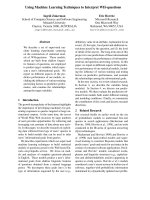
accessible. An ASC system usually operates in two main steps and depicted in Fig. 1.1.
Therefore, ASC systems have been researched and developed to replace the human

performing classification tasks. The first step is extracting the appropriate features of
the audio signals for use in the classifiers. The second step is to design a classification
model to implement classification tasks and have achieved certain achievements in
several ASC fields such as speech/music recognition and music transcription.

Fig. 1.1. The main framework of an ASC system
ASC is a field of audio data processing and is applied in entertainment, media,
education, digital libraries, and supervisor systems. Classical problems such as speech
and speaker recognition have been widely considered for decades [1]. In speech
recognition, audios are phonologically differentiated. Words, phrases, and sentences
are formed by combining these phonemes. The challenge is the ability to recognize
speech continuously, not grammatically and independently of the speaker. Another

1

FCU e-Theses & Dissertations (2021)


Audio Signal Classification Using Deep Learning Techniques

aspect of the ASC is music recognition and transcription [2, 3]. In this regard, the
acoustic signal is music, layers can be musical notes, and the output is usually a track.
Several systems were developed to address this, but the problem becomes more
complicated when the sound is full of orchestration. A more general ASC system can
distinguish between speech and music and can be used to assign sounds to a specific
transcription system. If a sound signal were classified as speech, speech recognition is
used, and if it were music, the music transcriber is called into action. In a system like
this, the speech recognizer and music transcriber can be optimized to expect the
appropriate input, simplify each, and improve the whole system's robustness. In
addition, there are other studies in the field of ASC, such as language recognition [46], audio context recognition [7], video segmenting based on audio [8], and sound

effects retrieval [9]. Each application is researched and developed separately and is only
applicable to a specific ASC problem. So there are still many issues that need to be
explored and added to the ASC fields.
1.2. Literature review
There are many studies regarding the methods and techniques applied in ASC in the
last decade. In 2005, Lin et al. [10] implemented a support vector machine (SVM) on
audio features such as subband power, pitch information, and frequency cepstral
coefficients, to perform audio categorization and classification. Audio feature
extraction and a multigroup classification system focusing on recognizing
discriminatory time-frequency subspaces employing the local discriminant bases
technique were introduced by Umapathy et al. [11] in 2007. Based on linear prediction
and linear prediction cepstral coefficients, a clustering algorithm was used to structure
the music content by Xu et al. [12]. Ajmera et al. [13] provided an approach that uses
an artificial neural network (ANN) and hidden Markov model (HMM) toward highperformance speech/music distinction on practical tasks correlated to the automatic
transcription of broadcast news. A technique was introduced for speech/music
discrimination based on root mean square and zero-crossings, as described in [14].
Another method was introduced by Honda et al. [15] for evaluating the distance of
single-channel audio signals; here, the signal's distance was evaluated by phase
interference within the observed and pseudo-observed signal waves.

2

FCU e-Theses & Dissertations (2021)


Audio Signal Classification Using Deep Learning Techniques

ANNs are gaining wide attention in recent years with the perceptron algorithm [16]
in 1957, the backpropagation algorithm [17] in 1986, and finally, the achievement of
deep learning (DL) in image classification [18] and speech recognition [19] in 2012. In

DL models, architectures with multiple layers connecting the input and output layers, a
large number of parameters are trained to learn from a big enough dataset is utilized.
Several basic architectures of DL networks usually used in ASC include multilayer
perceptions (MLPs), convolution neural networks (CNNs), and recurrent neural
networks (RNNs).
DL first gained attraction in image processing [18] but was then widely applied in
speech, music, environmental noise, and localization and tracking [20]. With the
achievement of DL models in speech recognition, other speech-related tasks also
embrace DL techniques, such as language recognition [21], speech translation [22], and
voice activity detection [23]. In music, DL has been successfully applied to many music
processing tasks and accelerating industrial applications with automatic descriptions for
browsing large catalogs, cabinet-based music recommendations content without using
data, and auto-derived chords for a song to play with. Due to its less common use in
environmental sound, the database is also more limited than speech and music. Most
open datasets have been published in the context of annual Detection and Classification
of Acoustic Scenes and Events [24]. In localization and tracking, DL has been used to
estimate the sound source distances [25] and localize a sound source [26]. In addition,
the DL also has applications such as heart sound classification [27], lung sound
classification [28], and fault diagnosis [29]. Most of the mentioned studies used
spectrogram and waveform of the audio signal fed to DL models such as CNNs, RNNs,
and CRNNs for the classification task and have superior performance compared to
traditional methods such as Gaussian mixture models, HMMs, and non-negative matrix
factorization [30]. The mentioned researches show the massive potential of DL and the
challenges posed to solving problems in ASC.
In summary, DL has been successfully applied to ASC tasks and accelerates the
development of industrial applications. However, most studies only perform a specific
task with a dataset. There are still many open issues for further studies, such as building
richer databases, what extraction features to use, and choosing and building the optimal
models for the best results. Along with that, the scope of applications in engineering
also needs to be expanded.


3

FCU e-Theses & Dissertations (2021)


Audio Signal Classification Using Deep Learning Techniques

1.3. Objectives
This work's main goal is to develop optimal DL models, including architecture and
setting parameters, and apply them to solve engineering problems related to sound
classification. Along with these goals, specific problems have been addressed, as
follows:
First, the two main processes in ASC, feature extraction and the machine learning
(ML) models are summarized. In which features and models used in DL are analyzed
and emphasized.
Second, a sound receiver location estimation method using a CNN was present. To
perform the proposed method, the simulation and experiment have been conducted and
achieved high accuracy. The research can also be applied to obtain optimal sound
quality and design of an audio room.
Third, a method to detect the abnormalities in water pumps based on sound analysis
using a DL technique was proposed. Experiments were conducted on three different
water pumps during suction from and discharge to the water tank under normal and
abnormal operating conditions. The results can be used to develop automatic pump fault
detection systems.
Finally, two DL models were proposed for heart sound classification based on the
log-mel spectrogram of heart sound signals. The results showed higher performance
than previous studies and can help cardiologists diagnose cardiovascular diseases.
1.4. Structure of this thesis
The structure of this thesis is as follows: Chapter 2 describes the methodologies in

detail. Three application studies of sound classifications using DL techniques were
conducted and discussed in Chapters 3, 4, and 5. Finally, Chapter 6 summarizes current
work with limitations and prospects for future work. As follows:
Chapter 2 presents the methodologies used in this thesis with the challenges
considered in Section 1.2. To be more detailed, a comprehensive study on audio
features and classification models is investigated for ASC. In which DL features and
models are emphasized and analyzed in detail.

4

FCU e-Theses & Dissertations (2021)


Audio Signal Classification Using Deep Learning Techniques

Chapter 3 presents the proposed method and experiment for sound receiver location
estimation using a CNN. In chapter 4, a method to detect the abnormalities in a machine
was proposed based on sound analysis using a DL technique, apply to water pump fault
detection. In chapter 5, two DL models of classifying heart sounds are proposed and
implemented to diagnose five heart valve diseases.
Chapter 6 summarizes and concludes the current work. The limitations are also
discussed to show out some potential directions for future work.

5

FCU e-Theses & Dissertations (2021)


Audio Signal Classification Using Deep Learning Techniques


Chapter 2
METHODOLOGY
This chapter presents the methodology applied in ASC. Usually, there are two main
steps to developing an ASC system: extracting features and building the classification
model. After being preprocessed for consistent format and noise reduction, the audio
signals will extract the necessary features in the time domain and frequency domain.
These features are then fed into the classifier as input. The classifier will be trained
based on the extraction features. Eventually, an unknown signal can be classified using
the trained model.
2.1. Audio features for ASC
2.1.1. Time-domain features
2.1.1.1.Short-term energy
Short-term energy is the average energy per window/frame [31] and computed
by Eq. (2.1).

E(i) =

1
N

[x (n)]

(2.1)

where x (n), n = 1,2, … , N is the sequence of a sound sample of the ith frame, and N
is the frame's length.
2.1.1.2. Loudness
Loudness is a property of an audio signal that determines the intensity of the
auditory sensation. Mathematically, loudness (in dB) is approximately proportionate to
the logarithm of sound intensity and expressed as

L = 10log

I
I

(2.2)

where I is the intensity of the sound signal and I = 10

W/m is the minimum

intensity detectable by the human ear.
Loudness has been employed in speech/music discrimination [32] and speech
segmentation [33].

6

FCU e-Theses & Dissertations (2021)


Audio Signal Classification Using Deep Learning Techniques

2.1.1.3. Temporal centroid
The temporal centroid is a temporal balancing point of sound energy. It can be
computed from the envelope of the signal across audio samples [34]. The temporal
centroid was applied in acoustic scene classification [35] and environmental sound
recognition [36].
2.1.1.4. Zero-Crossing Rate
Zero-crossing rate (ZCR) is the number of times of zero-crossing of an audio
signal within frame [31]. It can be expressed as:


ZCR =

1
2(L − 1)

|sgn[x(k + 1)] − sgn[x(k)]|

(2.3)

Eq. (2.4) expressed the sign function and x(k) is a discrete signal, k = 1 … L, L is
frame’s length.
−1 if x < 0
sgn(x) = 0 if x = 0
1 if x > 0

(2.4)

The ZCR is the measure of the general frequency content of an audio signal. It
is instrumental in distinguishing audio signals in the duration of the voiced and
unvoiced audio classes. As speech signals are commonly composed of alternating
voiced and unvoiced signals, which is not the case in music signals, the ZCR values'
variation is expected to be more significant for speech than for music. ZCR is often
applied in speech/music discrimination[37], musical genre classification [38], speech
analysis [39], and singing voice detection in music [40] because of its discriminative
energy in assigning speech, music, and various audio effects.
2.1.1.5. Entropy of Energy
The entropy of energy e represents abrupt changes in an audio signal's energy
level [31]. To compute e , each short-term frame is segmented into L sub-frames with
a fixed length. Then, each sub-frame's energy is calculated as in Eq. (2.1) and divided

by the total energy as in Eq. (2.5). Finally, the entropy H(i) of the sequence e is
calculated in Eq. (2.6) .

7

FCU e-Theses & Dissertations (2021)


Audio Signal Classification Using Deep Learning Techniques

e =

E
∑

(2.5)

E

H(i) = −

e . log e

(2.6)

Several researchers have used the entropy of energy in detecting the onset of
abrupt sounds, e.g. [41, 42].
2.1.2. Frequency – domain features
2.1.2.1.Spectral Centroid
The spectral centroid measures spectral position and shape, is the center of gravity

of the spectrum [31]. It has a strong relationship with the impression of brightness. The
spectral centroid C of a sound and calculated as
C =

∑

f(k)x(k)
∑
x(k)

(2.7)

where x(k) is the weighted frequency value and f(k) is the center frequency of bin
number k.
The spectral centroid has been applied in digital audio and music processing as
an automatic measure of musical timbre [43].
2.1.2.2. Spectral Entropy
Spectral entropy is determined similar to the entropy of energy, but the
computation occurs in the frequency domain [31]. In order to compute the spectral
energy, firstly, we divide the spectrum of the short-term frame into L sub-bands (bins).
The energy E of the fth bin, f = 0, … , L − 1, is then normalized by the cumulative
spectral energy in Eq. (2.8). Finally, the entropy of the normalized spectral energy f is
determined according to Eq. (2.9).
n =

H=−

E
∑


E

n . log (n )

8

(2.8)

(2.9)

FCU e-Theses & Dissertations (2021)


Audio Signal Classification Using Deep Learning Techniques

Spectral entropy was applied for efficiently discriminating between speech and
music in [44, 45].
2.1.2.3. Spectral Flux
Spectral flux represents the variability of the spectrum over time. Its
computation is the squared difference between the normalized magnitudes of the two
continuous short-term windows' spectra.. In order to compute the spectral flux, firstly,
we compute the kth normalized discrete Fourier transform (DFT) coefficient EN (k) at
the ith frame in Eq. (2.10). The spectral flux Fl ,

is then computed according to Eq.

(2.11).
x (k)

EN (k) =

∑

Fl ,

=

(2.10)

x (l)

EN (k) − EN

(2.11)

(k)

Spectral flux was applied in ASC such as speech [46], music genre [47], and
environmental sound [48].
2.1.2.4. Spectral roll-off
Spectral roll-off is the frequency below which a specific percentage (commonly
from 85% to 95%) of audio signal energy is intensive. If the mth DFT coefficient
correlates with to the spectral roll-off, then Eq. (2.12) is satisfied.

s = C.

s

(2.12)

where s is the spectral value at bin k , f and f are band edges, and C is the adopted

percentage.
Spectral roll-off has been applied in ASC such as speech/music [49] and music
genre [47, 50].
2.1.2.5. Mel-Frequency Cepstrum Coefficients
Mel-Frequency Cepstrum Coefficients (MFCCs) are obtained from the cepstral
representation of a signal [51]. MFCCs represent the short-term power spectrum of

9

FCU e-Theses & Dissertations (2021)


Audio Signal Classification Using Deep Learning Techniques

signal based on the discrete cosine transform of the log power spectrum on a non-linear
mel scale. The frequency bands are evenly ranged on Mel-scale, mimicking the human
auditory system very closely, making MFCCs key features in many signal processing
applications. The approximation of Mel-scale is expressed as
f

= 2595log

1+

where f is the physical frequency in Hz, and f

f
700

(2.13)


is the perceived frequency.

MFCCs were employed in ASC such as speech recognition [52, 53], speech
enhancement [54], music genre classification [55], music information retrieval [56],
audio similarity measurement [57], vowel detection [58], etc.
2.1.2.6. Spectrogram
A spectrogram is computed based on the fast Fourier transform (FFT) over
overlapping windows extracted from the sound signal. The sound signal's dividing
process in short-term sequences of fixed size and applying FFT is called Short-time
Fourier transform (STFT). The spectrogram is then calculated as the complex
magnitude of the STFT. Based on [59], the STFT of a sound signal x(n) with angular
frequency ω is defined as
X (mL, ω) = ∑

x(n) w(mL − n)e

(2.14a)

where the subscript w in X (mL, ω) denotes the analysis window w(n). L is an integer
that denotes the separation in time between adjacent short-time sections. For a fixed
value of m, X (mL, ω) represents the Fourier transform with respect to n of the shorttime section f (n) = x(n)w(mL − n).
In addition, a discrete STFT is defined as
X (mL, k) = X (mL, ω)|

/

(2.14b)

where N is the number of discrete frequencies. Finally, the spectrogram in logarithmic

scale is defined as
S(mL, k) = log|X (mL, k)|

(2.15)

Spectrogram has been applied widely in ASC, such as music classification [60],
language identification [61], and acoustic scene classification [62], etc.

10

FCU e-Theses & Dissertations (2021)


Audio Signal Classification Using Deep Learning Techniques

2.2. Classification models
2.2.1. Traditional machine learning models
In this section, the traditional models in ML are introduced. These models are
based on a simple analytical approach and can be adequate for classification
assignments with limited data sizes.
2.2.1.1. Näıve Bayes
Näıve Bayes (NB) is an algorithm based on employing Bayes’ theory with the
“naive” assumption of conditional independence between every pair of features
provided the value of the class variable [63]. Bayes’ theory states the resulting
relationship, given class variable y and dependent feature vector (x , … , x ):
P(y|x , … , x ) =

P(y)P(x , … , x |y)
P(x , … , x )


(2.16)

Due to over-simplified assumptions, the NB needs small training data to
determine the essential parameters. However, these algorithms have worked quite well
in actual tasks such as document classification [64] and spam filtering [65].
2.2.1.2. K-Nearest Neighbor
K-Nearest Neighbor (KNN) is a simple supervised learning algorithm applied
in regression and classification tasks but is mostly used for classification tasks [66].
KNN categorizes a new data point based on comparison with existing archived data and
puts the new case on the most similar available categories. Usually, the nearest neighbor
is determined based on Euclidean distance, which computed as the root of squared
differences between n-dimensional coordinates of two data points:

D x ,x

= D x ,x

=

x, −x,

(2.17)

The advantages of KNN are simple, robust with noisy training data, and high
efficiency with big data. The disadvantage of KNN is the high computational cost
because of calculating the distance for all training data samples.
2.2.1.3. Decision Tree

11


FCU e-Theses & Dissertations (2021)


Audio Signal Classification Using Deep Learning Techniques

Decision Tree (DT) is a tree-structured applied in both regression and
classification tasks, but it is mainly used for classification tasks [67]. Fig. 2.1 illustrates
the architecture of a DT example. In DT, decision nodes represent the dataset's features,
branches present decision rules, and the leaf nodes represent the outcomes. The
decisions or tests are performed based on the selected features of the given dataset. In
a DT, to predict the class of a data sample, the algorithm starts at the root node of the
tree and compares the root attribute values with the record attribute. Based on a
comparison, the algorithm follows a branch to goes to the following node. At the
following node, the algorithm again compares the characteristic value with other subnodes and moves further. This process will be complete when it reaches a leaf node.

Fig. 2.1. DT architecture example
Compared with other algorithms, DT has the advantages of being simple and
easy to understand, and has lower requirements for data cleaning. The disadvantage of
DT, however, is that it has many layers, making it complicated and may have an
overfitting issue, which can be improved by using the Random Forest (RF) algorithm.
2.2.1.4. Random Forest
RF is a classification model that contains many DTs on different subsets of the
provided dataset and takes the average to increase the dataset's predictive efficiency
[68]. Fig. 2.2 illustrates the RF prediction process. Instead of relying on a single tree's
prediction results, the RF synthesizes the predicted results from the trees and, based on
the prediction with a majority of votes, produces the final outcome. The more

12

FCU e-Theses & Dissertations (2021)



Audio Signal Classification Using Deep Learning Techniques

significant number of trees in the forest leads to higher efficiency and prevents
overfitting.
Compared with DT, the advantages of RF are that it has higher accuracy and
avoids overfitting problems if the number of trees is large enough [69]. However, this
algorithm's limitation is that a large number of trees increases computation time and is
not efficient for real-time prediction.

Fig. 2.2. RF prediction process example
2.2.1.5. Support vector machine
SVM aims to generate the best line or decision boundary that can separate ndimensional space into categories to put the new data point in the valid class quickly.
This best boundary or region is called a hyperplane. As illustrated in Fig. 2.3, the SVM
algorithm finds the support vectors that are the closest point from both classes' lines.
The distance from the support vectors to the hyperplane is called margin, and SVM
aims to maximize this margin. The hyperplane with the maximum margin is called the
optimal hyperplane. Two types of SVMs are linear SVM, which is applied in linearly
separable data, and nonlinear SVM, applied in nonlinearly separable data.

13

FCU e-Theses & Dissertations (2021)


Audio Signal Classification Using Deep Learning Techniques

Fig. 2.3. An SVM model in a binary classification problem.
The advantages of SVM are working almost well when there are a clear margin

of division between classes, high dimensional spaces, and the amount of dimensions is
larger than the number of samples. The disadvantages of SVM are not proper for big
data sets and performs not so well with noise datasets.
2.2.2. Deep learning models
DNNs are stratified neural networks, like interconnected neurons in the human
brain [70]. These networks operate in a cascade structure, with layers on the path
connected to allow data to flow. A back-propagation technique changes the weights
between the nodes in the network to ensure input data leads to correct output. DL
models can achieve greater accuracy and performance than traditional machine learning
models and are trained using a big dataset and a multi-layered neural network
architecture. In this thesis, three DL models are MLPs, CNNs, and RNNs, were
introduced.
2.2.2.1. Multilayer Perceptrons
MLP is a feed-forward network with connected neurons (nodes) feeding
forward from one layer to the next [71]. As shown in Fig. 2.4, an MLP consists of the
input layer, output layer, and hidden layers. The input layer gets the input data for
processing, while the output layer contains the predictions or classification results. One
or more hidden layers located between the input and output layers is the right matching
engine of the MLP. In an MLP, the data flows from the input to the output layer in the
forward direction. The associated weights are adjusted when the neurons are trained by
the back-propagation learning algorithm. MLPs are developed to approximate any

14

FCU e-Theses & Dissertations (2021)


Audio Signal Classification Using Deep Learning Techniques

continuous function and can solve nonlinear problems. MLP is mainly applied in ASC

such as pattern classification, recognition, prediction, and approximation.

Fig. 2.4. An example of MLPs’ architecture
The output

of an n-layer network with input x can be described as follow:
y = f(

where

f(

… f(

x +b )+⋯+b

)+b )

is the associated weight matrix with the ith layer, the vector

(2.18)
(i = 1,2, … n)

represents the bias values for each node in ith layer, and f is the nonlinear activation
function. Some typical activation functions are the sigmoid function (sigmoid), the
hyperbolic tangent function (tanh), and the rectified linear unit function (ReLU). Eqs
define these functions are Eqs. (2.19a-2.19c) and Fig. 2.5 depicts their plot.
sigmoid x

=


e
1+e

(2.19a)

e
e

−1
+1

(2.19b)

tanh(x) =

ReLU(x) = max(x, 0)

15

(2.19c)

FCU e-Theses & Dissertations (2021)