Microstrip Antennas Part 4 doc
Bạn đang xem bản rút gọn của tài liệu. Xem và tải ngay bản đầy đủ của tài liệu tại đây (1.95 MB, 30 trang )
Particle-Swarm-Optimization-Based Selective Neural Network Ensemble
and Its Application to Modeling Resonant Frequency of Microstrip Antenna
79
No f
ME
[3] [4] [5] [6] [7] [8] [9] [10] [11] [12] [13]
1 7740 7804 7697 7750 7791 7635 7737 7763 7720 7717 412 7765
2 8450 8496 8369 8431 8478 8298 8417 8446 8396 8389 488 8451
3 3970 4027 3898 3949 3983 3838 3951 3950 3917 3887 510 3977
4 7730 7940 7442 7605 7733 7322 7763 7639 7551 7376 1610 7730
5 4600 4697 4254 4407 4641 4455 4979 4759 4614 4430 113 4618
6 5060 5283 4865 4989 5070 4741 5101 4958 4924 4797 1621 5077
7 4805 5014 4635 4749 4824 4520 4846 4724 4688 4573 1460 4830
8 6560 6958 6220 6421 6566 6067 6729 6382 6357 6114 2550 6563
9 5600 5795 5270 5424 5535 5158 5625 5414 5374 5194 1769 5535
10 6200 6653 5845 6053 6201 5682 6413 5987 5988 5735 2860 6193
11 7050 7828 6566 6867 7052 6320 7504 6682 6769 6433 4792 7030
12 5800 6325 5435 5653 5801 5259 6078 5552 5586 5326 3259 5787
13 5270 5820 4943 5155 5287 4762 5572 5030 5081 4842 3383 5273
14 7990 9319 7334 7813 7981 6917 8885 7339 7570 6822 8674 8101
15 6570 7412 6070 6390 6550 5794 7076 6135 6264 5951 5486 6543
16 5100 5945 4667 4993 5092 4407 5693 4678 4830 4338 5437 5193
17 8000 8698 6845 7546 7519 6464 8447 6889 7160 6367 8067 7948
18 7134 7485 5870 6601 6484 5525 7342 5904 6179 5452 7242 7169
19 6070 6478 5092 5660 5606 4803 6317 5125 5341 4735 6103 6026
20 5820 6180 4855 5423 5352 4576 6042 4886 5100 4513 5875 5817
21 6380 6523 5101 5823 5660 4784 6453 5122 5396 4729 6546 6515
22 5990 5798 4539 5264 5063 4239 5804 4550 4830 4196 5976 6064
23 4660 4768 3746 4227 4141 3526 4689 3770 3949 3479 4600 4613
24 4600 4084 3201 3824 3615 2938 4209 3168 3446 2921 4603 4550
25 3580 3408 2668 3115 2983 2485 3430 2670 2845 2461 3574 3628
26 3980 3585 2808 3335 3162 2590 3668 2790 3015 2572 3955 3956
27 3900 3558 2785 3299 3133 2573 3629 2771 2987 2555 3895 3907
28 3980 3510 2753 3294 3112 2522 3626 2721 2966 2509 3982 3922
29 3900 3313 2608 3147 2964 2364 3473 2554 2823 2356 3903 3747
30 3470 3001 2358 2838 2675 2146 3129 2317 2549 2137 3493 3381
31 3200 2779 2183 2623 2474 1992 2889 2151 2357 1983 3197 3123
32 2980 2684 2102 2502 2370 1936 2752 2086 2259 1924 2982 2972
33 3150 2763 2168 2600 2453 1982 2863 2139 2338 1972 3160 3096
Errors 13136 24097 11539 12322 30669 8468 22572 18148 30504 56698 1393
Resonant frequencies and errors are in MHz.
Table 6. Resonant frequency obtained from traditional methods for rectangular MSAs and
sum of absolute errors between experimental results and theoretical results
Microstrip Antennas
80
conventional methods [3]-[13] are listed in table 6. The sum of absolute errors between
experimental and theoretical results for every method is also listed in the last row of table 6.
It is clear from table 5 and table 6 that the computing results of the chaos BiPSO-based
selective NNE are better than these of previously proposed methods, which proves the
validity of the algorithm further.
7. Conclusion
Selective neural network ensemble (NNE) methods based on decimal particle swarm
optimization (DePSO) algorithm and binary particle swarm optimization (BiPSO) algorithm
are proposed in this study. In these algorithms, optimally select neural networks (NNs) to
construct NNE with the aid of particle swarm optimization (PSO) algorithm, which can
maintain the diversity of NNs. In the process of ensemble, the performance of NNE may be
improved by appropriate restriction on combination weights based on BiPSO algorithm.
And this may avoid calculating the matrix inversion and decrease the multi-dimensional
collinearity and the over-fitting problem of noise. In order to effectively ensure the particles
diversity of PSO algorithm, chaos mutation is adopted during the iteration process
according to randomicity, ergodicity and regularity in chaos theory. Experimental results
show that the chaos BiPSO algorithm can improve the generalization ability of NNE. By
using the chaos BiPSO-based selective NNE, resonant frequency of rectangular microstrip
antenna (MSA) is modeled, and the computing results are better than available ones, which
mean that the proposed NNE in this study is effective. The method of NNE proposed in this
study may be conveniently extended to other microwave engineering and designs.
8. Acknowledge
This work is supported by Pre-research foundation of shipping industry of China under
grant No. 10J3.5.2, and Natural Science Foundation of Higher Education of Jiangsu Province
of China under grant No. 07KJB510032.
9. Reference
[1] Wong K L, “Compact and broadband microstrip antennas”, New York: John Wiley & Sons
Inc., 2002.
[2] Kumar G, and Ray K P, “Broadband microstrip antennas”, MA: Artech House, 2003.
[3] Howell J Q, “Microstrip antennas”, IEEE Transactions on Antennas and Propagation, 1975,
23(1): 90-93.
[4] Hammerstad E O, “Equations for microstrip circuits design”, Proc. 5th Eur. Microw.
Conf., Hamburg, Germany, Sep. 1975, pp. 268–272.
[5] Carver K R, “Practical analytical techniques for the microstrip antenna”, Proc. Workshop
Printed Circuit Antenna Tech., New Mexico State Univ., Las Cruces, NM, Oct. 1979,
pp. 7.1–7.20.
[6] Bahl I J, and Bhartia P, “Microstrip Antennas”, MA: Artech House, 1980.
[7] James J R, Hall P S, and Wood C, “Microstrip antennas-theory and design”, London:
Peregrinus, 1981.
[8] Sengupta D L, “Approximate expression for the resonant frequency of a rectangular
patch antenna”, Electronics Letters, 1983, 19: 834-835.
Particle-Swarm-Optimization-Based Selective Neural Network Ensemble
and Its Application to Modeling Resonant Frequency of Microstrip Antenna
81
[9] Garg R, and Long S A, “Resonant frequency of electrically thick rectangular microstrip
antennas”, Electronics Letters, 1987, 23: 1149-1151.
[10] Chew W C, and Liu Q, “Resonance frequency of a rectangular microstrip patch”, IEEE
Transactions on Antennas Propagation, 1988, 36: 1045-1056.
[11] Guney K, “A new edge extension expression for the resonant frequency of electrically
thick rectangular microstrip antennas”, Int. J. Electron., 1993, 75: 767-770.
[12] Kara M, “Closed-form expressions for the resonant frequency of rectangular microstrip
antenna elements with thick substrates”, Microwave and Optical Technology
Letters,1996, 12: 131-136.
[13] Guney K, “A new edge extension expression for the resonant frequency of rectangular
microstrip antennas with thin and thick substrates”, J. Commun. Tech. Electron.,
2004, 49: 49-53.
[14] Zhang Q J, and Gupta K C, “Neural networks for RF and microwave design”, MA: Artech
House, 2000.
[15] Christodoulou C, and Georgiopoulos M, “Applications of Neural Networks in
Electromagnetic”, MA: Artech House, 2001.
[16] Guney K, Sagiroglu S, and Erler M, “Generalized neural method to determine resonant
frequencies of various microstrip antennas”, International Journal of RF and
Microwave Computer-Aided Engineering, 2002, 12(1): 131-139.
[17] Sagiroglu S, and Kalinli A, “Determining resonant frequencies of various microstrip
antennas within a single neural model trained using parallel tabu search
algorithm”, Electromagnetics, 2005, 25(6): 551-565.
[18] Kara M, “The resonant frequency of rectangular microstrip antenna elements with
various substrate thicknesses”, Microwave and Optical Technology Letters, 1996, 11:
55-59.
[19] Hansen L K, and Salamon P, “Neural network ensembles”, IEEE Transactions on Pattern
Analysis and Machine Intelligence, 1990, 12(10): 993-1001.
[20] Kennedy J, and Eberhart R C, “Particle Swarm Optimization”, IEEE International
Conference on Neural Networks, Piscataway, NJ: IEEE Press, 1995, 1942-1948.
[21] Zeng J C, Jie J, and Cui Z H, “Particle swarm optimization”, Beijing: Science Press, 2004.
[22] Clerc M, “Particle Swarm Optimization”, ISTE Publishing Company, 2006.
[23] R. Poli. Analysis of the publications on the applications of particle swarm optimization.
Journal of Artificial Evolution and Applications, 2008, Article No. 4.
[24] Robinson J, and Rahmat-Samii Y, “Particle swarm optimization in electromagnetics”,
IEEE Transactions on Antennas and Propagation, 2004, 52(2): 397-407.
[25] Mussetta M, Selleri S, Pirinoli P, et al., “Improved Particle Swarm Optimization
algorithms for electromagnetic optimization”, Journal of Intelligent and Fuzzy
Systems, 2008, 19(1): 75-84.
[26] M. T. Hagan, H. B. Demuth, and M. H. Beale, Neural Network Design, Boston: PWS
Pub. Co., 1995.
[27] S. Haykin. Neural Networks: A Comprehensive Foundation (2nd Edition), Prentice
Hall, 1999.
[28] Y. B. Tian, Hybrid neural network techniques, Beijing: Science Press, 2010.
[29] Merz C J, and Pazzani M J, “A principal components approach to combining regression
estimates”, Machine Learning, 1999, 36 (1-2): 9-32.
Microstrip Antennas
82
[30] Hashem S, “Treating harmful collinearity in neural network ensembles”, In: Sharkey A J
C, ed. Combining artificial neural nets: Ensemble and modular multi2net systems,
Great Britain: Springer-Verlag London Limited, 1999. 101-123.
[31] Zhou Zhihua, Wu Jianxin, and Tang Wei, “Ensembling neural networks: Many could be
better than all”, Artificial Intelligence, 2002, 137 (1-2): 239-263.
[32] Dietterich T G, “An experimental comparison of three methods for constructing
ensembles of decision trees: Bagging, boosting, and randomization”, Machine
Learning, 2000, 40: 139-157.
[33] Kennedy J, and Eberhart R, “A discrete binary version of the particle swarm
optimization”, Proceedings IEEE International Conference on Computational
Cybernetics and Simulation. Piscataway, NJ: IEEE, 1997: 4104-4108.
[34] Huang R S, and Huang H, “Chaos and its applications”, China Wuhan: Wuhan University
press, 2005.
[35] Zhang L P, “Theory and applications of particle swarm optimization”, Ph. D. dissertation,
Zhejiang University, China, 2005.
[36] Shi Y, and Eberhart R, “Empirical study of particle swarm optimization”, Proceedings
of the 1999 Congress on Evolutionary Computation, 1999: 1945-1950.
5
Microstrip Antennas Conformed onto
Spherical Surfaces
Daniel B. Ferreira and J. C. da S. Lacava
Technological Institute of Aeronautics
Brazil
1. Introduction
Microstrip antennas are customary components in modern communications systems, since
they are low-profile, low-weight, low-cost, and well suited for integration with microwave
circuits. Antennas printed on planar surfaces or conformed onto cylindrical bodies have
been discussed in many publications, being the subject of a variety of analytical and
numerical methods developed for their investigation (Josefsson & Persson, 2006; Garg et al.,
2001; Wong, 1999). However, such is not the case of spherical microstrip antennas and
arrays composed of these radiators. Even commercial electromagnetic software, like HFSS
®
and CST
®
, do not provide a tool to assist the design of spherical antennas and arrays, i.e.,
electromagnetic simulators do not have an estimator tool for establishing the initial
dimensions of a spherical microstrip antenna for further numerical analysis, as available for
planar geometries. Moreover, this software is time-consuming when utilized to simulate
spherical radiators, hence it is desirable that the antenna geometry to be analyzed is not too
far off from the final optimized one, otherwise the project cost will likely be affected.
Nonetheless, spherical microstrip antenna arrays have a great practical interest because they
can direct a beam in an arbitrary direction throughout the space, i.e., without limiting the
scan angles, differently from the planar antenna behaviour. This characteristic makes them
feasible for use in communication satellites and telemetry (Sipus et al., 2006), for example.
Rigorous analysis of spherical microstrip antennas and their respective arrays has been
conducted through the Method of Moments (MoM) (Tam et al., 1995; Wong, 1999; Sipus et
al., 2006). But the MoM involves highly complex and time-consuming calculations. On the
other hand, whenever the objective is the analysis of spherical thin radiators, the cavity
model (Lima et al., 1991) can be applied, instead of the MoM. However, for both MoM and
cavity model, the behaviour of the antenna input impedance and radiated electric field is
described by the associated Legendre functions, hence efficient numerical routines for their
evaluation are required, otherwise the scope of the antennas analyzed is restricted.
In order to overcome the drawbacks described above, a Mathematica
®
-based CAD software
capable of performing the analysis and synthesis of spherical-annular and -circular thin
microstrip antennas and their respective arrays with high computational efficiency is
presented in this chapter. It is worth mentioning that the theoretical model utilized in the
CAD can be extended to other canonical spherical patch geometries such as rectangular or
triangular ones. The Mathematica
®
package, an integrated scientifical computing software
with a vast collection of built-in functions, was chosen mainly due to its powerful
Microstrip Antennas
84
algorithms for calculating cylindrical and spherical harmonics functions what makes it
suitable for the analysis of conformed antennas. Mathematica
®
permits the analysis and
synthesis of various spherical microstrip radiators, thus avoiding the use of the normalized
Legendre functions that are sometimes employed to overcome numerical difficulties (Sipus
et al., 2006). Furthermore, it is important to point out that the developed CAD does not
require a powerful computer to run on, working well and quickly in a regular classroom PC,
since its code does not utilize complex numerical techniques, like MoM or finite element
method (FEM). In Section 2, the theoretical model implemented in the developed CAD to
evaluate the antenna input impedance, quality factor, radiation pattern and directivity is
discussed. Furthermore, comparisons between the CAD results and the HFSS
®
full wave
solver data are presented in order to validate the accuracy of the utilized technique.
An effective procedure, based on the global coordinate system technique (Sengupta, 1968),
to determine the radiation patterns of thin spherical meridian and circumferential arrays is
utilized in the special-purpose CAD, as addressed in Section 3. The array radiation patterns
so obtained with the CAD are also compared to those from the HFSS
®
software. Section 4 is
devoted to present an alternative strategy for fabricating a low-cost spherical-circular
microstrip antenna along with the respective experimental results supporting the proposed
antenna fabrication approach.
2. Analysis and synthesis of spherical thin microstrip antennas
The geometry of a probe-fed spherical-annular microstrip antenna embedded in free space
(electric permittivity ε
0
and magnetic permeability μ
0
) is shown in Fig. 1. It is composed of a
metallic sphere of radius a, called ground sphere, covered by a dielectric layer (ε and μ
0
) of
thickness h = b – a.
z
a
x
y
Metallic
sphere
Dielectric
layer
Probe
position
h
Annular
patch
1
θ
p
θ
2
θ
b
z
a
x
y
Metallic
sphere
Dielectric
layer
Probe
position
h
Annular
patch
1
θ
p
θ
2
θ
b
Fig. 1. Geometry of a probe-fed spherical-annular microstrip antenna.
A symmetrical annular metallic patch, defined by the angles θ
1
and θ
2
(θ
2
> θ
1
> 0), is fed by
a coaxial probe positioned at (θ
p
, φ
p
). The radiators treated in this chapter are electrically
thin, i.e., h << λ (λ is the wavelength in the dielectric layer), so the cavity model (Lo et al.,
Microstrip Antennas Conformed onto Spherical Surfaces
85
1979) is well suited for the analysis of such antennas. Based on this model it is possible to
develop expressions for computing the antenna input impedance and for estimating the
electric surface current density on the patch without employing any complex numerical
method such as the MoM.
Before starting the input impedance calculation, the expression for computing the resonant
frequencies of the modes established in a lossless equivalent cavity is determined. In the
case of electrically thin radiators, the electric field within the cavity can be considered to
have a radial component only, which is r-independent. Therefore, applying Maxwell’s
equations to the dielectric layer region, and disregarding the feeder presence, the following
equation for the r-component of the electric field is obtained
2
2
2222
11
sin 0
sin sin
rr
r
EE
kE
aa
∂∂∂
⎛⎞
θ
++=
⎜⎟
∂θ ∂θ
θθ∂φ
⎝⎠
, (1)
where k
2
= ω
2
μ
0
ε and ω denotes the angular frequency. Consequently, only TM
r
modes can
be established in the equivalent cavity.
Solving the wave equation (1) via the method of separation of variables (Balanis, 1989),
results in the electric field
( , ) [ P (cos ) Q (cos )][ cos( ) sin( )]
θ
φ= θ+ θ φ+ φ
AA
mm
r
EA B CmDm, (2)
where
P(.)
A
m
and
Q(.)
A
m
are the associated Legendre functions of ℓ-th degree and m-th order
of the first and the second kinds, respectively, ℓ(ℓ +1) = k
2
a
2
and A, B, C and D are constants
dependent on the boundary conditions.
Enforcing the boundary conditions related to the equivalent cavity of annular geometry and
taking into account that it is symmetrical in relation to the z-axis, the electric field (2)
reduces to
(,) R(cos)cos( )
θ
φ= θ φ
AA
m
r
m
EE m, (3)
where
11 1
R (cos ) sin [P (cos )Q (cos ) Q (cos )P (cos )]
mmmmm
cc c
′′
θ
=θ θ θ− θ θ
AAAAA
, (4)
m = 0, 1, 2,… and the index ℓ must satisfy the transcendental equation
12 12
P (cos )Q (cos ) Q (cos )P (cos ) 0
mm mm
cc cc
′′ ′′
θ
θ− θ θ=
AA AA
, (5)
with the angles θ
1c
and θ
2c
(θ
2c
> θ
1c
) indicating the equivalent cavity borders in the θ
direction, i.e., θ
1c
≤ θ ≤ θ
2c
, 0 ≤ φ < 2π, E
ℓm
are the coefficients of the natural modes and the
prime denotes a derivative. Hence, once the indexes ℓ and m are determined it is possible to
evaluate the TM
ℓm
mode resonant frequency from the following expression
0
(1)
2
m
f
a
+
=
π
με
A
AA
. (6)
Before solving the transcendental equation (5) it is necessary to determine the equivalent
cavity dimensions θ
1c
and θ
2c
, which correspond to the actual patch dimensions with the
Microstrip Antennas
86
addition of the fringe field extension. However, differently from planar microstrip antennas,
the literature does not currently present expressions for estimating the dimensions of
spherical equivalent cavities based on the physical antenna dimensions and the dielectric
substrate characteristics. Therefore, in this chapter, the expressions used for estimating the
equivalent cavity dimensions of a planar-annular microstrip antenna are extended to the
spherical-annular case (Kishk, 1993), i.e., the spherical-annular equivalent cavity arc lengths
were considered equal to the respective linear dimensions of the planar-annular equivalent
cavity. The proposed expressions are given below; equations (7.a) and (7.b),
1
11
1
2F( )
1
c
r
h
b
θ
θ=θ −
π
θε
, (7.a)
2
22
2
2F( )
1
c
r
h
b
θ
θ=θ +
π
θε
, (7.b)
where
F( ) n( /2 ) 1.41 1.77 (0.268 1.65) /
rr
bh h bθ= θ + ε+ + ε+ θA and ε
r
is the relative electric
permittivity of the dielectric substrate.
2.1 Input impedance
The input impedance of the spherical-annular microstrip antenna illustrated in Fig. 1 fed by a
coaxial probe can be evaluated following the procedure proposed in (Richards et al., 1981), i.e.,
the coaxial probe is modelled by a strip of current whose electric current density is given by,
()
2
1
ˆ
,()()
sin
p
f
p
JJr
a
θφ = φδθ−θ
θ
G
, (8)
where δ(.) indicates the Dirac’s delta function and
0
,if /2 /2
()
0, otherwise
pp
J
J
φ −Δφ ≤φ≤φ +Δφ
⎧
⎪
φ=
⎨
⎪
⎩
(9)
with Δφ denoting the strip angular length relative to the φ−direction. In our analysis, also
following the procedure established in (Richards et al., 1981) for planar microstrip antennas,
the strip arc length has been assumed to be five times the coaxial probe diameter d,
expressed as
5/sin
p
da
Δ
φ= θ . (10)
It is important to point out that the electric current density (8) is an r-independent function
since the antenna under analysis is electrically thin. Thus, to take into account the current
strip, the wave equation (1) for the electric field is modified to
()
2
2
0
2222
11
ˆ
sin ,
sin sin
rr
rf
EE
kE j J r
aa
∂∂∂
⎛⎞
θ
++=ωμθφ⋅
⎜⎟
∂θ ∂θ
θθ∂φ
⎝⎠
G
. (11)
Expanding the r-component of the electric field into its eigenmodes (3), the solution for
equation (11) is given by
Microstrip Antennas Conformed onto Spherical Surfaces
87
1
00
2cos
22 2
cos
R (cos )sinc( /2)cos( )
( , ) R (cos )cos( )
[][R()]
c
c
m
p
p
m
r
m
m
m
m
mm
J
Ej m
a
kk d
2
θ
ν= θ
θΔφ φ
ωμ Δφ
θφ = θ φ
π
ξ− νν
∑∑
∫
A
A
A
AA
, (12)
where
2, if 0
1, otherwise
m
m =
⎧
ξ=
⎨
⎩
,
(1)/
m
ka=+
A
AA
and sinc(x)=sin(x)/x.
Since the procedure just described has been developed for ideal cavities, equation (12) is
purely imaginary. So, for incorporating the radiated power and the dielectric and metallic
losses into the cavity model, the concept of effective loss tangent, tan
δ
eff
, (Richards et al.,
1979) is employed. Based on this approach, the wave number k is replaced by an effective
wave number
1tan
eff eff
kk j
=
−δ. (13)
Once the electric field inside the equivalent cavity has been determined, the antenna input
voltage V
in
can be computed from the expression,
in r
VEh=− , (14)
where
r
E denotes the average value of (,)
p
r
E
θ
φ over the strip of current. Consequently, the
input impedance Z
in
of the spherical-annular microstrip antenna is given by
1
22 2
0
2cos
22 2
0
cos
[R (cos )] sinc ( /2)cos ( )
[ (1 tan )] [R ( )]
c
c
m
p
p
in
in
m
m
meff
m
mm
Vh
Zj
J
a
kk j d
2
θ
ν= θ
θΔφφ
ωμ
==
Δφ
π
ξ
−−δ νν
∑∑
∫
A
A
AA
. (15)
An alternative representation for frequencies close to the TM
LM
resonant mode but
sufficiently apart from the other modes can be obtained by rewriting the antenna input
impedance as
2222
(, )(, )
(1 tan )
LM
m
in
LM eff
m
m
mLM
j
Zj
j
≠
α
ωα
≅+ω
ω
−− δω ω−ω
∑
∑
A
A
A
A
, (16)
where
1
cos
22 2 2 2
cos
[R (cos )] sinc ( / 2)cos ( ) / [R ( )] .
c
c
m m
p
pm
m
hmma d
2
θ
ν= θ
α= θ Δφ φ πεξ ν ν
∫
AA A
The expression (16) corresponds to the equivalent circuit shown in Fig. 2, i.e., a parallel RLC
circuit with a series inductance L
p
. In this case, the series inductance represents the probe
effect and its value is that of the double sum in (16). However, as this is a slowly convergent
series, the developed CAD utilizes, alternatively, the equation due to (Damiano & Papiernik,
1994) for calculating the probe reactance X
p
, given by
0
60 n( /2)
p
Xjkhkd
=
− A , (17)
Microstrip Antennas
88
where
000
k =ω μ ε and provided
0
0.2kd
<
< .
in
Z
p
L
R
L
C
in
Z
p
L
R
L
C
p
L
R
L
C
Fig. 2. Simplified equivalent circuit for thin microstrip antennas.
The previous expressions developed for computing the resonant frequencies and the input
impedance of spherical-annular microstrip antennas can also be used for analysing
wraparound radiators. However, in the limit case when θ
1
→ 0, i.e., the antenna patch
corresponding to a circular one (Fig. 3), the associated Legendre function of the second kind
becomes unbounded for θ → 0, so it is no longer part of the function that describes the
electromagnetic field within the equivalent cavity. So, to obtain the expressions for
spherical-circular microstrip antennas it is enough to eliminate the Legendre function of the
second kind from the previously developed solution for spherical-annular antennas. These
expressions are presented in Table 1. In Section 2.3 examples are given for spherical-annular
and -circular microstrip antennas.
Resonant frequency
0
(1)
2
m
f
a
+
=
π
με
A
AA
, the index ℓ is obtained from P
2
(cos ) 0
m
c
′
θ=
A
Input impedance
1
22 2
0
2cos
22 2
cos
[P (cos )] sinc ( / 2)cos ( )
[ (1 tan )] [P ( )]
c
c
m
p
p
in
m
m
meff
m
mm
h
Zj
a
kk j d
2
θ
ν= θ
θΔφφ
ωμ
=
π
ξ
−−δ νν
∑∑
∫
A
A
AA
Table 1. Spherical-circular microstrip antenna expressions.
z
a
Metallic
sphere
Dielectric
layer
Probe
position
h
Circular
patch
2
θ
b
x
y
p
θ
z
a
Metallic
sphere
Dielectric
layer
Probe
position
h
Circular
patch
2
θ
b
x
y
p
θ
Fig. 3. Geometry of a probe-fed spherical-circular microstrip antenna.
Microstrip Antennas Conformed onto Spherical Surfaces
89
2.2 Radiated far electric field
In the developed CAD, the electric surface current method (Tam & Luk, 1991) is used to
determine the far electric field radiated by the thin spherical-annular and -circular
microstrip antennas. This method is very convenient in the case of spherical-annular and -
circular patches since both are electrically symmetrical. As a result, no numerical integration
is required for the calculation of the spectral current density and the radiated power.
Moreover, differently from planar and cylindrical geometries, where truncation of the
ground layer and diffraction at the edges of the conducting surfaces affect the radiation
patterns, thin spherical microstrip patches of canonical geometries can be efficiently
analyzed by combining the cavity model with the electric surface current method.
The procedure proposed here starts from observing that the geometry shown in Fig 1 (or in
Fig. 3) can be treated as a three-layer structure, made out of ground, dielectric substrate and
free space. Consequently, its spectral dyadic Green’s function, necessary for calculating the
far electric field via the electric surface current method, can be easily evaluated using an
equivalent circuital model (Giang et al., 2005). As it is based on the (
ABCD) matrix
(transmission matrix) concept,
Mathematica
®
’s symbolic capability can be used for
calculating the matrices involved. The technique for establishing the structure’s equivalent
circuital model and, consequently, its spectral dyadic Green’s function is presented next.
The fields within the dielectric layer can be written as the sum of TE
r
and TM
r
modes with
the aid of the vector auxiliary potential approach (Balanis, 1989). In this case, the expressions
for the transversal components of the electromagnetic field are given by
P
(1) (2)
||
||
11
ˆˆ
(,,) H ( ) H ( ) (cos)
mm m
nn nn n
mnm
d
Er A kr B kr
rd
j
+∞ +∞
θ
0
=−∞ =
⎧
⎪
′′
⎡⎤
θ
φ= + θ
⎨
⎢⎥
⎣⎦
θ
με
⎪
⎩
∑∑
P
(1) (2)
||
ˆˆ
H() H() (cos) ,
sin
jm
mmm
nn nn n
m
CkrDkr e
j
φ
⎫
⎪
⎡⎤
++ θ
⎬
⎣⎦
εθ
⎪
⎭
(18)
P
(1) (2)
||
||
1
ˆˆ
(,,) H ( ) H ( ) (cos )
sin
mmm
nn nn n
mnm
m
Er A kr B kr
r
+∞ +∞
φ
0
=−∞ =
⎧
⎪
′′
⎡⎤
θ
φ= + θ
⎨
⎢⎥
⎣⎦
με θ
⎪
⎩
∑∑
P
(1) (2)
||
1
ˆˆ
H() H() (cos) ,
jm
mm m
nn nn n
d
CkrDkr e
d
φ
⎫
⎡⎤
++ θ
⎬
⎣⎦
εθ
⎭
(19)
P
(1) (2)
||
||
1
ˆˆ
(,,) H ( ) H ( ) (cos)
sin
mmm
nn nn n
mnm
jm
Hr A kr B kr
r
+∞ +∞
θ
0
=−∞ =
⎧
⎪
⎡⎤
θ
φ= + θ
⎨
⎣⎦
μθ
⎪
⎩
∑∑
P
(1) (2)
||
1
ˆˆ
H() H() (cos) ,
jm
mm m
nn nn n
d
CkrDkr e
d
j
φ
0
⎫
⎪
′′⎡⎤
++ θ
⎬
⎢⎥
⎣⎦
θ
με
⎪
⎭
(20)
P
(1) (2)
||
||
11
ˆˆ
(,,) H ( ) H ( ) (cos)
mm m
nn nn n
mnm
d
Hr A kr B kr
rd
+∞ +∞
φ
0
=−∞ =
⎧
⎪
⎡⎤
θ
φ= − + θ
⎨
⎣⎦
μθ
⎪
⎩
∑∑
Microstrip Antennas
90
P
(1) (2)
||
ˆˆ
H() H() (cos) ,
sin
jm
mmm
nn nn n
m
CkrDkr e
φ
0
⎫
⎪
′′⎡⎤
++θ
⎬
⎢⎥
⎣⎦
με θ
⎪
⎭
(21)
where the coefficients
m
n
A ,
m
n
B ,
m
n
C and
m
n
D are dependent on the boundary conditions at the
interfaces r
= a and r = b, and
τ()
ˆ
H(.)
n
is the Schelkunoff spherical Hankel function of n-th order
and τ-th kind (τ = 1 or 2). The fields (18) to (21) can be rewritten in a more adequate form as
||
(, ,) (,) ,
jm
mnm
E
Lnm rne
E
+∞ +∞
θ
φ
φ
=−∞ =
⎡⎤
=θ⋅
⎢⎥
⎣⎦
∑∑
G
E
(22)
||
(, ,) (,) ,
jm
mnm
H
Lnm rne
H
+∞ +∞
θ
φ
φ
=−∞ =
⎡⎤
=θ⋅
⎢⎥
⎣⎦
∑∑
G
H
(23)
where
P
P
P
P
||
||
||
||
(cos )
(cos )
sin
(, ,) ,
(cos )
(cos )
sin
m
m
n
n
m
m
n
n
d
jm
d
Lnm
d
jm
d
⎡
⎤
θ
θ−
⎢
⎥
θθ
⎢
⎥
θ=
⎢
⎥
θ
θ
⎢
⎥
θθ
⎣
⎦
(24)
(1) (2)
(1) (2)
ˆˆ
H() H()
(, ) ,
1
ˆˆ
H() H()
mm
nn nn
mm
nn nn
AkrBkr
jkr
rn
CkrDkr
r
θ
φ
ω
⎡
⎤
′′
⎡
⎤
+
⎢
⎥
⎢
⎥
⎣
⎦
⎡⎤
⎢
⎥
==
⎢⎥
⎢
⎥
⎣⎦
⎡
⎤
+
⎢
⎥
⎣
⎦
ε
⎣
⎦
G
E
E
E
(25)
(1) (2)
(1) (2)
ˆˆ
H() H()
(, )
1
ˆˆ
H() H()
mm
nn nn
mm
nn nn
CkrDkr
jkr
rn
AkrBkr
r
θ
φ
0
ω
⎡
⎤
′′
⎡
⎤
+
⎢
⎥
⎢
⎥
⎣
⎦
⎡⎤
⎢
⎥
==
⎢⎥
⎢
⎥
⎣⎦
⎡
⎤
−+
⎢
⎥
⎣
⎦
μ
⎣
⎦
G
H
H
H
, (26)
and the argument (r,θ,φ) was omitted in (22) and (23) only for simplifying the notation. The
vectors
G
(, )rnE
and
G
(, )rnH
are the transversal electric and magnetic fields in the spectral
domain, respectively. In this chapter, the pair of vector-Legendre transforms (Sipus et al.,
2006) is defined as follows,
ππ
−φ
φ= θ=
=
θ⋅ θφ θ θφ
π
∫∫
GG
2
00
1
(, ) (, ,) (,,)sin
2(,)
jm
rn Lnm Xr e dd
Snm
X (27)
and
||
(,,) (, ,) (, ) ,
jm
mnm
Xr Lnm rne
+∞ +∞
φ
=−∞ =
θφ = θ⋅
∑∑
G
G
X (28)
Microstrip Antennas Conformed onto Spherical Surfaces
91
where ( , ) 2 ( 1)( | |)!/(2 1)( | |)!Snm nn n m n n m=++ +− and ( , )rn
G
X , the vector-Legendre
transform of ( , , )Xr
θ
φ
G
, has only the θ and/or φ components.
From evaluating the expressions (25) and (26) at the lower (r
= a) and upper (r = b) interfaces
it is possible to establish the following relation
(,) (,)
,
(,) (,)
VZ
an bn
YB
an bn
⎡
⎤⎡⎤
⎡⎤
=⋅
⎢
⎥⎢⎥
⎢⎥
⎢⎥
⎢
⎥⎢⎥
⎣⎦
⎣
⎦⎣⎦
G
G
GG
EE
HH
(29)
and the matrices
V
, Z
, Y
and B
can be found in (Ferreira, 2009).
Based on equation (29), the two-port network illustrated in Fig. 4, representing the dielectric
layer, can be defined. The related transmission (
ABCD) matrix is given in (30).
G
H b,n()
G
E b,n()
G
H a,n()
G
E a,n()
VZ
YB
⎡
⎤
⎢
⎥
⎢
⎥
⎣
⎦
G
H b,n()
G
E b,n()
G
H a,n()
G
E a,n()
VZ
YB
⎡
⎤
⎢
⎥
⎢
⎥
⎣
⎦
Fig. 4. Transmission (
ABCD) network.
() .
VZ
ABCD
YB
⎡
⎤
=
⎢
⎥
⎢
⎥
⎣
⎦
(30)
In a similar way, the following relation between the free-space spectral electric
0
G
E and
magnetic
0
G
H transversal field components can be determined,
000
(,) (,),bn Y bn=⋅
G
G
HE (31)
where
(2) (2)
000
0
(2) (2)
00 0
ˆˆ
0H()/H()
,
ˆˆ
H( )/ H ( ) 0
nn
nn
kb
j
kb
Y
kb j kb
′
⎡
⎤
η
⎢
⎥
=
′
⎢
⎥
η
⎣
⎦
(32)
and η
0
denotes the free space intrinsic impedance. Consequently, free space can be
represented by the admittance load
0
Y
in the circuital model. It is worth mentioning that the
matrices
V
, Z
, Y
, B
and
0
Y
can be evaluated in a straightforward manner utilizing the
Mathematica
®
’s symbolic capability.
As the ground layer is considered a perfect electric conductor, it is well represented by a
short circuit that corresponds to null electric field (
0
g
=
G
E ). On the other hand, the spectral
electric surface current density
s
G
J located on the metallic patch is modelled by an ideal
current source. The circuital representations for both short circuit and ideal current source
are given in Fig. 5.
Finally, by properly combining the circuit elements, the three-layer structure model is the
equivalent circuit illustrated in Fig. 6, whose resolution produces the transversal dyadic
Green’s function
G
in the spectral domain. Notice that the Green’s function, calculated
according to this approach, is evaluated at the dielectric substrate – free space interface
(
r = b).
Microstrip Antennas
92
0
g
=
G
E 0
g
=
G
E
G
H b,n()
G
J
s
0
G
H b,n()
G
H b,n()
G
J
s
0
G
H b,n()
(a) (b)
Fig. 5. Short circuit (a) and ideal current source (b) circuital representations.
G
H b,n()
G
E b,n()
G
H a,n()
G
E a,n()
VZ
YB
⎡
⎤
⎢
⎥
⎢
⎥
⎣
⎦
G
J
s
0
~
Y
0
G
H b,n()
0
G
E b,n()
G
H b,n()
G
E b,n()
G
H a,n()
G
E a,n()
VZ
YB
⎡
⎤
⎢
⎥
⎢
⎥
⎣
⎦
G
J
s
0
~
Y
0
G
H b,n()
0
G
E b,n()
Fig. 6. Circuital representation for the spherical three-layer structure.
It is important to point out that the Mathematica
®
’s symbolic capability is also helpful for the
circuit resolution and allows writing the related functions in a compact form, as shown:
0
(,) ,
s
bn G
=
⋅
G
G
EJ
(33)
where
0
(,)
0
G
GGbn
G
θ
θ
φφ
−
⎡
⎤
==
⎢
⎥
⎣
⎦
, (34)
(2)
00
(2) (2)
00
ˆ
H( )
ˆˆ
(H()H())
nn
rn n n n
qkb
G
jp kbq kb
θθ
′
η
=
′
ε+
, (35)
(2)
00
(2) (2)
00
ˆ
H( )
ˆˆ
H( ) H ( )
nn
rn n n n
js kb
G
rkbs kb
φφ
η
=
′
ε+
, (36)
with
(2) (1) (1) (2)
ˆˆ ˆˆ
H ( )H ( ) H ( )H ( ),
nn n n n
p
kb ka kb ka
′′
=− (37.a)
(2) (1) (1) (2)
ˆˆ ˆˆ
H ()H()H()H(),
nn n n n
q
ka kb ka kb
′′ ′′
=− (37.b)
(2)(1) (1)(2)
ˆˆ ˆˆ
H ( )H ( ) H ( )H ( ),
nn n n n
rkakbkakb
′′
=− (37.c)
(2) (1) (1) (2)
ˆˆ ˆˆ
H ( )H ( ) H ( )H ( )
nn n n n
skbkakbka=− (37.d)
and
T
ss sφθ
⎡⎤
=−
⎣⎦
G
JJ J
whose superscript T indicates the transpose operator.
Microstrip Antennas Conformed onto Spherical Surfaces
93
Writing the free-space spectral electric field (r > b) as a function of the field evaluated at the
dielectric substrate – free space interface (r
= b) and taking the asymptotic expression (r → ∞)
for the Schelkunoff spherical Hankel function of second kind and n-th order (Olver, 1972),
the spectral far electric field is derived as
0
0
(, ) ,
j
kr
n
s
e
rn jbAG
r
−
≅⋅⋅
G
G
EJ (38)
where
(2)
1
0
(2)
1
0
ˆ
[H ( )] 0
.
ˆ
0[H()]
n
n
kb
A
jkb
−
−
⎡
′⎤
⎢
⎥
=
⎢
⎥
⎣
⎦
So, applying (28) to the spectral field (38), the spatial far electric field radiated from the
spherical microstrip antenna is determined,
0
||
(, ,) .
j
kr
jm
n
s
mnm
E
e
jbLnm AG e
E
r
+∞ +∞
−
θ
φ
φ
=−∞ =
⎡⎤
=θ⋅⋅⋅
⎢⎥
⎣⎦
∑∑
G
J (39)
Notice that the present development did not take into account the patch geometry, since the
electric surface current density has not been specified yet. Hence, expression (39) can be
applied to any arbitrary patch geometry conformed onto the structure of Fig. 1, and not only
to the annular or circular ones. However, as this chapter’s purpose is to develop a
computationally efficient CAD for the analysis of thin spherical-annular and -circular
microstrip antennas, instead of employing a complex numerical method, such as the MoM,
for determining the electric surface current densities on the patches, the cavity model was
enough for their accurate estimation. Following this approach for the case of the spherical-
annular patch operating in the TM
LM
mode, the expressions below are obtained
0
R (cos )cos( ),
M
LM
sL
Ed
Jj M
ad
θ
=
−θφ
ωμ θ
(40.a)
0
R(cos)sin( ).
sin
M
LM
sL
ME
Jj M
a
φ
=
θφ
ωμ θ
(40.b)
So, after the vector-Legendre transform, the spectral components of the surface current
density can be evaluated in closed form as,
2
11 1
0
2
22 2
(1)
[sin P (cos )R (cos )
2(,)(1)(1)
sin P (cos )R (cos )],
MM
LM
scncLc
MM
cn c L c
ELL
j
aS n M n n L L
θ
+
′
=θθθ
ωμ + − +
′
−θ θ θ
J
(41.a)
22 11
0
[P (cos )R (cos ) P (cos )R (cos )],
2(,)
MM MM
LM
s n cL c n cL c
mE
aS n M
φ
=θθ−θθ
ωμ
J (41.b)
if m = M or m = – M. Otherwise, 0
s
=
G
J . Consequently the expression for the far electric field
radiated by this radiator is also determined in closed form.
Microstrip Antennas
94
In a similar way, expressions for the spatial and spectral electric surface current densities are
derived for the spherical-circular microstrip antenna (Fig. 3) operating in the TM
LM
mode
0
P (cos )cos( ),
M
LM
sL
Ed
Jj M
ad
θ
=
−θφ
ωμ θ
(42.a)
0
P(cos)sin( ),
sin
M
LM
sL
ME
Jj M
a
φ
=
θφ
ωμ θ
(42.b)
2
22 2
0
(1)
sin P (cos )P (cos ),
2(,)(1)(1)
MM
LM
scncLc
jE
LL
aS n M n n L L
θ
−
+
′
=θθθ
ωμ + − +
J (43.a)
22
0
P(cos )P(cos ),
2(,)
MM
LM
sncLc
mE
aS n M
φ
=θθ
ωμ
J (43.b)
if m = M or m = – M. Otherwise, 0
s
=
G
J .
Once the far electric field radiated by spherical antennas is known, an expression for its
average radiated power can be established. Starting from equation (44) (Balanis, 2005),
2
*2
0
0
00
1
sin ,
2
PEErdd
ππ
φ= θ=
=
⋅θθφ
η
∫∫
GG
(44)
where
E
G
denotes the far electric field determined by (39) and the superscript * indicates the
complex conjugate operator. After the double integration, the following expression can be
obtained
2
2
2
0
(2)
(2)
0
0
||
0
(, ) .
ˆ
ˆ
H( )
H( )
s
s
n
mnm
n
G
G
b
PSnm
kb
kb
+∞ +∞
φφφ
θθθ
=−∞ =
⎡
⎤
π
⎢
⎥
=+
⎢
⎥
′
η
⎢
⎥
⎣
⎦
∑∑
J
J
(45)
In order to calculate the directivity of thin spherical-annular and -circular microstrip
antennas, the developed CAD employs (45), since its evaluation requires no numerical
integrations, which, as previously mentioned, is an advantage. In addition, equation (45) is
employed in the CAD for computing the quality factor associated to the radiated power,
from which the effective loss tangent tan
δ
eff
and, consequently, the antenna input
impedance (15) are estimated.
2.3 CAD results
Before presenting some CAD results and comparing them with HFSS
®
output data, a brief
overview of the CAD structure will be given. The current version of the CAD contains two
independent sections: the synthesis and the analysis modules that can be accessed from their
respective tabs. By selecting the Synthesis option, the design interface (Fig. 7) is presented.
The inputs required for the synthesis procedure to start are the desired frequency, the
ground sphere radius a and the substrate parameters, such as relative permittivity
ε
r
, loss
tangent tan
δ and thickness h. As results, the CAD returns the patch physical dimensions (θ
1
and
θ
2
for the annular patch and only θ
2
for the circular one) and the probe position θ
p
Microstrip Antennas Conformed onto Spherical Surfaces
95
considering the antenna fed by a 50-ohm SMA connector at φ
p
= 0°. The Analysis module
evaluates the electromagnetic characteristics of a synthesized antenna. The inputs required
for the analysis procedure to start are the metallic sphere radius a, the substrate parameters,
the patch angular dimensions and the probe position. As outputs, the antenna input
impedance (rectangular plot), quality factor, radiation patterns (polar plots) and directivity
are calculated. Notice that the window illustrated in Fig. 7 is relative to the spherical-circular
microstrip antenna; another similar one was developed for the spherical-annular radiator.
Fig. 7. The Synthesis module interface.
The CAD algorithm was implemented in Mathematica
®
mainly due to the efficient numerical
routines for the computation of the associated Legendre functions. Besides, Mathematica
®
has a vast collection of built-in functions that permit implementing the respective code in a
short number of lines, plus its many graphical resources.
In order to solve the transcendental equation and to calculate the equivalent cavity resonant
frequencies in a fast and accurate way, the CAD utilizes a set of interpolation polynomials
specially developed to provide seed values for the Mathematica
®
’s numerical routine that
searches the transcendental equation root in a given operation mode. The interpolation
polynomials were calculated based on graphical analysis, so the CAD can determine the
resonant frequency of a specific mode without any further graphical inspection. For
example, the interpolation polynomial associated to the TM
11
mode of a spherical-circular
cavity which is employed by the CAD is:
22334
11 2 2 2 2 2
65 76 87 108
222 2
( ) 54.46 11.06 1.13 6.21 10 1.67 10
5.36 10 8.71 10 2.07 10 1.53 10 ,
ccccc
ccc c
−−
−− −−
θ
=−θ+θ−×θ+×θ
−
×θ−×θ+×θ−× θ
A
(46)
where
θ
2c
is given in degrees.
Microstrip Antennas
96
To illustrate the CAD synthesis procedure, a spherical-circular antenna conformed onto a
typical microwave laminate (
ε
r
= 2.5, loss tangent = 0.0022 and h = 0.762 mm) fed by a 50-ohm
SMA coaxial connector of 0.65-mm radius, was designed to operate at 2.1 GHz. The radius of
the metallic sphere is a =100 mm. After entering these parameters, the CAD outputs
θ
2
= 14.92
degrees and
θ
p
= 4.47 degrees, in a few minutes of computational time, even running on a
regular classroom desktop computer. The input data and the results are automatically saved
for use in the analysis module. In Fig. 8, the comparison is shown between the radiation
patterns, at the operating frequency, obtained from the developed CAD and from the HFSS
®
package for the spherical-circular microstrip antenna so designed. It is seen that the radiation
patterns exhibit excellent agreement, thus validating our procedure to calculate the radiated
far electric field based on the combination of the cavity model with the electric surface current
method. It is important to point out that HFSS
®
employs the FEM (finite element method) for
solving high frequency structures, so it takes considerable time to determine the structure
solution. In addition, it does not provide an estimator tool to establish the initial geometry of
the spherical radiator as the developed CAD does.
Results for the real and imaginary parts of the antenna input impedance are presented in
Fig. 9; once again, the curves are very similar.
-30
-20
-10
0
0°
30°
60°
90°
120°
150°
180°
210°
240°
270°
300°
330°
-30
-20
-10
0
CAD
HFSS
[dB]
E
θ
radiation pattern: xz plane.
-30
-20
-10
0
0°
30°
60°
90°
120°
150°
180°
210°
240°
270°
300°
330°
-30
-20
-10
0
CAD
HFSS
[dB]
E
φ
radiation pattern: yz plane.
Fig. 8. Comparison between the radiation patterns.
The half power quality factor Q and the antenna directivity D shown in Table 2 are also in
very good agreement.
CAD HFSS
®
Deviation
Q
78.8 80.8 2.5%
D (dB) 6.6 6.9 0.3 dB
Table 2. Quality factor and directivity.
As another illustrative example, a spherical-annular antenna fed by a 50-ohm SMA coaxial
connector of 0.65-mm radius and conformed onto the same typical microwave laminate
used before was designed to operate at 1.364 GHz in the TM
10
mode. In this case,
θ
1
= 10.0 degrees, θ
2
= 30.0 degrees, θ
p
= 13.21 degrees and the ground sphere has a radius
a = 200 mm. The radiation pattern in the E-plane, at 1.364 GHz, and the input impedance
curve evaluated in the CAD and HFSS
®
are presented in Figs. 10 and 11, respectively. It is
clear from these figures that, once again, the results are very similar.
Microstrip Antennas Conformed onto Spherical Surfaces
97
2.04 2.06 2.08 2.10 2.12 2.14 2.16
-30
-20
-10
0
10
20
30
40
50
60
Input impedance [Ω]
Frequency [GHz]
Re ( Z
in
) CAD
Im ( Z
in
) CAD
Re ( Z
in
) HFSS
Im ( Z
in
) HFSS
Fig. 9. Spherical-circular microstrip antenna input impedance.
-30
-20
-10
0
0°
30°
60°
90°
120°
150°
180°
210°
240°
270°
300°
330°
-30
-20
-10
0
CAD
HFSS
[dB]
Fig. 10. E
θ
radiation pattern: E-plane.
1.30 1.32 1.34 1.36 1.38 1.40 1.42
-10
-5
0
5
10
15
20
25
30
Input impedance [Ω]
Frequency [GHz]
Re ( Z
in
) CAD
Im ( Z
in
) CAD
Re ( Z
in
) HFSS
Im ( Z
in
) HFSS
Fig. 11. Spherical-annular antenna input impedance (TM
10
mode).
Microstrip Antennas
98
3. Radiation patterns of spherical arrays
As aforementioned, a great advantage of using spherical arrays is the possibility of 360°
coverage in any radial direction. So, they have potential application in tracking, telemetry
and command services for low-earth and medium-earth orbit satellites (Sipus et al., 2008).
Rigorous analysis of spherical microstrip antenna arrays has been carried out using the
MoM (Sipus et al., 2006). However, the MoM involves highly-complex and time-consuming
calculations even considering the far-field evaluation alone. On the other hand, when
spherical-annular or –circular patches of thin radiators are positioned symmetrically in
relation to the z-axis, they can be effectively analyzed through the electric surface current
method in association with the cavity model, as shown in Section 2. In case of spherical
arrays, not all array elements can be positioned symmetrically with respect to the z-axis.
Hence, in this chapter, the global coordinate system technique (Sengupta et al., 1968) is
employed to evaluate the far electric field radiated by each one of the array elements.
To illustrate the proposed technique, let’s analyze the spherical-circular microstrip antenna
shown in Fig. 12, which represents a generic spherical array element whose centre is located
at (
α
n
, β
n
).
α
n
x
y
z
β
n
'
z
'
x
'
y
a
h
α
n
x
y
z
β
n
'
z
'
x
'
y
a
h
Fig. 12. Geometry of a spherical-circular array element.
Starting from the expressions for the far electric field components E
θ
’
(.) and E
φ
’
(.) of a patch
that is symmetrically positioned around the z’-axis, as calculated in Section 2.2, and using
the global coordinate system, the following expressions for the radiated far electric field
components in the reference (r,
θ,φ) coordinate system are obtained
rot n n
EAEBE
′′
θθ φ
′
′′′
θ
φ= θφ − θφ( , ) ( , ) ( , ), (47)
rot n n
EBEAE
′′
φθ φ
′
′′′
θ
φ= θφ + θφ( , ) ( , ) ( , ), (48)
where
nnnn
A
′
=
−θα φ−β+θα θ[ cos sin cos( ) sin cos ] /sin , (49)
nn n
B
′
=
αφ−β θ[sin sin( )]/sin , (50)
with
Microstrip Antennas Conformed onto Spherical Surfaces
99
cos sin sin cos( ) cos cos
nnn
′
θ
=α θ φ−β+ α θ, (51)
and
cos sin cos( ) sin cos
cot .
sin sin( )
nnn
n
α
θφ−β−α θ
′
φ=
θφ−β
(52)
To verify this approach, a spherical-circular single-element antenna, such as the one
illustrated in Fig. 12, whose centre is positioned at (
α
n
= 30°, β
n
= 0°), was designed in our
CAD to operate at 3.1 GHz (TM
11
mode). The spherical-circular patch, fed at (θ
pn
= 27.1°,
φ
pn
= 0°) by a 50-ohm SMA coaxial connector of 0.65-mm radius, is conformed onto a
microwave laminate with
ε
r
= 2.5, loss tangent = 0.0022 and h = 0.762 mm. The radius of the
metallic sphere is a =100 mm. The designed antenna was also simulated in HFSS
®
package
for comparison purposes. Fig. 13 shows the results obtained from the CAD for the radiation
patterns in xz- and yz-planes compared to those simulated in HFSS
®
. As observed, they
exhibit excellent agreement.
-30
-20
-10
0
0°
30°
60°
90°
120°
150°
180°
210°
240°
270°
300°
330°
-30
-20
-10
0
CAD
HFSS
[dB]
E
rot
θ
radiation pattern: xz plane.
-30
-20
-10
0
0°
30°
60°
90°
120°
150°
180°
210°
240°
270°
300°
330°
-30
-20
-10
0
CAD
HFSS
[dB]
E
rot
φ
radiation pattern: yz plane.
Fig. 13. Radiation patterns of the designed rotated element.
After validating the adopted procedure for calculating the radiation pattern of a generic
spherical array element, the array analysis can be carried out. Since for spherical arrays
there is no diffraction at the edges of the conducting surfaces and considering that coupling
among the array elements can be neglected for radiation pattern purposes, the components
of the far electric field radiated by an spherical array can be calculated by superposing the
fields radiated by each element individually. Following this approach, the components of
the far electric field radiated by a spherical array of N elements can be evaluated from
1
(,) ( , ) ( , ),
N
Rnn
n
EAEBE
′′
θθφ
=
′
′′′
θ
φ= θφ − θφ
∑
(53)
1
(,) ( , ) ( , ).
N
Rnn
n
EBEAE
′′
φθφ
=
′
′′′
θ
φ= θφ + θφ
∑
(54)
Microstrip Antennas
100
To illustrate the proposed procedure, an array consisting of two spherical-circular elements,
as shown in Fig. 14, was designed to operate at 3.1 GHz (TM
11
mode, ε
r
= 2.5, tan δ = 0.0022,
h = 0.762 mm and a = 100 mm). The antennas are fed by identical currents, β
1
= 0° and
β
2
= 180°. The patch spacing α was chosen to be 15° and 90°, one at time, in order to analyze
the developed approach for a wide range of α. Figs. 15 and 16 show the radiation patterns in
the xz- and yz-planes evaluated both with the CAD and HFSS
®
. As seen, they are in excellent
agreement, even in the case when the patches are closer together (α = 15°), thus validating
the adopted technique. In the next sections, two spherical arrays configurations are
discussed: the meridian-spherical and circumferential-spherical arrays whose radiation
patterns will be evaluated following this approach.
3.1 Meridian-spherical arrays
The geometry of the spherical-circular meridian array, i.e. one whose patches are all centred
along a constant-φ plane, is shown in Fig. 17. In this particular configuration, the array is
positioned along the φ = β plane and the patch centres are located at α
i
, where i = 1, 2, …, N.
Note the maximum number of elements N is a function of the sphere radius, the dielectric
permittivity and the operating frequency, in a way to avoid the superposition of patches.
1
2
α
x
z
α
h
a
1
2
α
x
z
α
h
a
Fig. 14. Two-element array: cut in xz-plane.
-30
-20
-10
0
0°
30°
60°
90°
120°
150°
180°
210°
240°
270°
300°
330°
-30
-20
-10
0
CAD
HFSS
[dB]
E
R
θ
radiation pattern: xz plane.
-30
-20
-10
0
0°
30°
60°
90°
120°
150°
180°
210°
240°
270°
300°
330°
-30
-20
-10
0
CAD
HFSS
[dB]
E
R
φ
radiation pattern: yz plane.
Fig. 15. Two-element array radiation patterns: α = 15º.
Microstrip Antennas Conformed onto Spherical Surfaces
101
-30
-20
-10
0
0°
30°
60°
90°
120°
150°
180°
210°
240°
270°
300°
330°
-30
-20
-10
0
CAD
HFSS
[dB]
E
R
θ
radiation pattern: xz plane.
-30
-20
-10
0
0°
30°
60°
90°
120°
150°
180°
210°
240°
270°
300°
330°
-30
-20
-10
0
CAD
HFSS
[dB]
E
R
φ
radiation pattern: yz plane.
Fig. 16. Two-element array radiation patterns: α = 90º.
1
α
x
y
z
2
α
α
N
1
2
N
1
α
x
y
z
2
α
α
N
11
22
NN
Fig. 17. Meridian-spherical array.
x
z
1
2
0
3
4
2
α
2
α
α
α
h
a
x
z
1
2
0
3
4
2
α
2
α
α
α
h
a
Fig. 18. Five-element array: cut in xz plane.
As an example of a spherical-circular meridian array, consider the five-element array shown
in Fig. 18. This array was also designed to operate at 3.1 GHz (TM
11
mode, ε
r
= 2.5,
tan δ = 0.0022, h = 0.762 mm and a = 100 mm) and its elements are fed by identical currents.
The uniform patch spacing α was chosen to be 27.5°. Results for the corresponding radiation
Microstrip Antennas
102
patterns, evaluated with both our CAD and HFSS
®
are illustrated in Fig. 19. Once again, the
radiation patterns are in very good agreement, thus demonstrating that the coupling
between the array elements can be neglected in the calculation of the far electric field the
array radiates.
-30
-20
-10
0
0°
30°
60°
90°
120°
150°
180°
210°
240°
270°
300°
330°
-30
-20
-10
0
CAD
HFSS
[dB]
E
R
θ
radiation pattern: xz plane.
-30
-20
-10
0
0°
30°
60°
90°
120°
150°
180°
210°
240°
270°
300°
330°
-30
-20
-10
0
CAD
HFSS
[dB]
E
R
φ
radiation pattern: yz plane.
Fig. 19. Five-element array radiation patterns.
3.2 Circumferential-spherical arrays
A circumferential-spherical array of N-element is shown in Fig. 20. In this case, the patches
are centred along a θ-constant cone and the maximum number of elements N is a function of
θ, the sphere radius a, the dielectric permittivity and the operating frequency, in a way to
avoid the superposition of patches.
To illustrate the analysis technique, let’s consider the four-element array presented in
Fig. 21. This array was also designed to operate at 3.1 GHz (TM
11
mode, ε
r
= 2.5,
tan δ = 0.0022, h = 0.762 mm and a = 100 mm) and its elements are fed by identical currents,
but α = 35º. Results for the radiation patterns in the xz- and yz-planes evaluated with both
the CAD and HFSS
®
are shown in Fig. 22. As seen from these results, the radiation patterns
are in excellent agreement, thus supporting the validation of the superposition procedure
presented in this chapter for the calculation of the far electric field radiated by spherical
microstrip antenna arrays.
α
x
y
z
1
N
1
β
N
β
2
α
α
x
y
z
11
NN
1
β
N
β
22
α
Fig. 20. Circumferential-spherical array.
Microstrip Antennas Conformed onto Spherical Surfaces
103
x
y
z
α
1
2
4
3
a
h
x
y
z
α
11
22
44
33
a
h
Fig. 21. Four-element circumferential array.
-30
-20
-10
0
0°
30°
60°
90°
120°
150°
180°
210°
240°
270°
300°
330°
-30
-20
-10
0
CAD
HFSS
[dB]
E
R
θ
radiation pattern: yz plane.
-30
-20
-10
0
0°
30°
60°
90°
120°
150°
180°
210°
240°
270°
300°
330°
-30
-20
-10
0
CAD
HFSS
[dB]
E
R
φ
radiation pattern: xz plane.
Fig. 22. Four-element array radiation patterns.
Although the examples given in this section involve spherical arrays whose patches are
circular, the proposed technique can be applied in the same manner to spherical arrays
whose patches are annular.
4. Prototype design and experimental results
The theoretical model developed in the previous sections considers the dielectric substrate
and the patch are both conformed onto the metallic ground sphere. Although the fabrication
of spherical-microstrip antennas starting from planar radiators is a very challenging task
(Piper & Bialkowski, 2004), the procedure can be eased if the geometry is slightly modified,
i.e., if a facet is cut on the metallic spherical layer for mounting a planar antenna. An
example of such modified geometry is illustrated in Fig. 23 where a planar circular patch is
mounted onto the facet. The same adaptation could be made for other patch geometries, as
the annular or rectangular, for instance. But, for this modified geometry, an essential
question is posed: how well can its electromagnetic behavior be predicted from the
theoretical model previously developed?
When the dimensions of the planar patch are much smaller than the metallic sphere radius,
the electrical characteristics of the hybrid geometry tend to those of an equivalent antenna
whose patch and dielectric substrate are conformed onto the ground sphere. So, the