22
Table 1.3
Fiscal Policy
A Demand Shock


Unemployment 0 Inflation 0
Shock in A 2 Shock in B
− 2
Unemployment 2 Inflation
− 2
Change in Govt Purchases 2
Unemployment 0 Inflation 0



Table 1.4
Fiscal Policy
A Supply Shock


Unemployment 0 Inflation 0
Shock in A 2 Shock in B 2
Unemployment 2 Inflation 2
Change in Govt Purchases 2
Unemployment 0 Inflation 4



Fiscal Policy

23
Chapter 3
Monetary and Fiscal Interaction



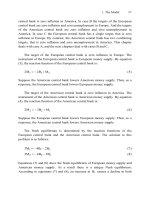
An increase in money supply lowers unemployment. On the other hand, it
raises inflation. Correspondingly, an increase in government purchases lowers
unemployment. On the other hand, it raises inflation. The target of the central
bank is zero inflation. By contrast, the target of the government is zero
unemployment.

The model of unemployment and inflation can be represented by a system of
two equations:


u = A M G−α −β
(1)

π B + αεM βεG=+
(2)

Of course this is a reduced form. Here
u
denotes the rate of unemployment,
π
is
the rate of inflation,
M is money supply, G is government purchases, α is the

monetary policy multiplier with respect to unemployment,
α
ε is the monetary
policy multiplier with respect to inflation,
β
is the fiscal policy multiplier with
respect to unemployment,
βε
is the fiscal policy multiplier with respect to
inflation,
A is some other factors bearing on the rate of unemployment, and B is
some other factors bearing on the rate of inflation. The endogenous variables are
the rate of unemployment and the rate of inflation.

According to equation (1), the rate of unemployment is a positive function of
A, a negative function of money supply, and a negative function of government
purchases. According to equation (2), the rate of inflation is a positive function of
B, a positive function of money supply, and a positive function of government
purchases. A unit increase in A raises the rate of unemployment by 1 percentage
point. A unit increase in B raises the rate of inflation by 1 percentage point. A
unit increase in money supply lowers the rate of unemployment by
α percentage
points. On the other hand, it raises the rate of inflation by
α
ε percentage points.
A unit increase in government purchases lowers the rate of unemployment by
β


M. Carlberg, Monetary and Fiscal Strategies in the World Economy, 23

DOI 10.1007/978-3-642-10476-3_4, © Springer-Verlag Berlin Heidelberg 2010

24
percentage points. On the other hand, it raises the rate of inflation by
β
ε

percentage points.

The target of the central bank is zero inflation. The instrument of the central
bank is money supply. By equation (2), the reaction function of the central bank
is:


M = B Gαε − − βε
(3)

Suppose the government raises its purchases. Then, as a response, the central
bank lowers money supply.

The target of the government is zero unemployment. The instrument of the
government is government purchases. By equation (1), the reaction function of
the government is:


βGAαM=−
(4)

Suppose the central bank lowers money supply. Then, as a response, the
government raises its purchases.


The Nash equilibrium is determined by the reaction functions of the central
bank and the government. From the reaction function of the central bank follows:


dM
dG
β
=−
α
(5)

And from the reaction function of the government follows:


dG
dM
α
=−
β
(6)

That is to say, the reaction curves do not intersect. As an important result, there is
no Nash equilibrium.

Monetary and Fiscal Interaction

25
Chapter 4
Monetary and Fiscal Cooperation


1. The Model



An increase in money supply lowers unemployment. On the other hand, it
raises inflation. Correspondingly, an increase in government purchases lowers
unemployment. On the other hand, it raises inflation. The policy makers are the
central bank and the government. The targets of policy cooperation are zero
inflation and zero unemployment.

The model of unemployment and inflation can be characterized by a system
of two equations:


u = A M G−α −β
(1)

π B + αεM βεG=+
(2)

Of course this is a reduced form. Here
u
denotes the rate of unemployment,
π
is
the rate of inflation,
M is money supply, G is government purchases, α is the
monetary policy multiplier with respect to unemployment,
α

ε is the monetary
policy multiplier with respect to inflation,
β
is the fiscal policy multiplier with
respect to unemployment,
βε
is the fiscal policy multiplier with respect to
inflation,
A is some other factors bearing on the rate of unemployment, and B is
some other factors bearing on the rate of inflation. The endogenous variables are
the rate of unemployment and the rate of inflation.

According to equation (1), the rate of unemployment is a positive function of
A, a negative function of money supply, and a negative function of government
purchases. According to equation (2), the rate of inflation is a positive function of
B, a positive function of money supply, and a positive function of government
purchases. A unit increase in A raises the rate of unemployment by 1 percentage
point. A unit increase in B raises the rate of inflation by 1 percentage point. A
unit increase in money supply lowers the rate of unemployment by
α percentage

M. Carlberg, Monetary and Fiscal Strategies in the World Economy, 25
DOI 10.1007/978-3-642-10476-3_5, © Springer-Verlag Berlin Heidelberg 2010

26
points. On the other hand, it raises the rate of inflation by
α
ε percentage points.
A unit increase in government purchases lowers the rate of unemployment by
β


percentage points. On the other hand, it raises the rate of inflation by
β
ε

percentage points.

The policy makers are the central bank and the government. The targets of
policy cooperation are zero inflation and zero unemployment. The instruments of
policy cooperation are money supply and government purchases. Thus there are
two targets and two instruments. We assume that the policy makers agree on a
common loss function:


22
Lu=π +
(3)

L is the loss caused by inflation and unemployment. For ease of exposition we
assume equal weights in the loss function. The specific target of policy
cooperation is to minimize the loss, given the inflation function and the
unemployment function. Taking account of equations (1) and (2), the loss
function under policy cooperation can be written as follows:


22
L(B M G) (A M G)=+αε+βε +−α−β (4)

Then the first-order conditions for a minimum loss are:



22
(1 ) M A B (1 ) G+ε α = −ε − +ε β (5)


22
(1 ) G A B (1 ) M+ε β = −ε − +ε α (6)

Equation (5) shows the first-order condition with respect to money supply. And
equation (6) shows the first-order condition with respect to government
purchases. Obviously, equations (5) and (6) are identical. There are two
endogenous variables, money supply and government purchases. On the other
hand, there is only one independent equation. Thus there is an infinite number of
solutions.

The cooperative equilibrium is determined by the first-order conditions for a
minimum loss. The solution to this problem is as follows:

Monetary and Fiscal Cooperation

27

2
AB
MG
1
−
ε
α+β=
+

ε
(7)

Equation (7) yields the optimum combinations of money supply and government
purchases. As a result, monetary and fiscal cooperation can reduce the loss
caused by inflation and unemployment.

From equations (1) and (7) follows the optimum rate of unemployment:


2
2
AB
u
1
ε+ε
=
+ε
(8)

And from equations (2) and (7) follows the optimum rate of inflation:


2
AB
1
ε+
π=
+ε
(9)


Unemployment is not zero, nor is inflation.
1. The Model

28
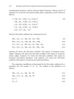
2. Some Numerical Examples



For ease of exposition we assume that monetary and fiscal policy multipliers
are unity
1α=β=ε=
. On this assumption, the model of unemployment and
inflation can be written as follows:

uAMG=−−
(1)
BMGπ= + +
(2)

A unit increase in A raises the rate of unemployment by 1 percentage point. A
unit increase in B raises the rate of inflation by 1 percentage point. A unit
increase in money supply lowers the rate of unemployment by 1 percentage
point. On the other hand, it raises the rate of inflation by 1 percentage point. A
unit increase in government purchases lowers the rate of unemployment by 1
percentage point. On the other hand, it raises the rate of inflation by 1 percentage
point. The model can be solved this way:

2M 2G A B+=−
(3)

2u A B=+
(4)
2ABπ= +
(5)

Equation (3) shows the optimum combinations of money supply and government
purchases, equation (4) shows the optimum rate of unemployment, and equation
(5) shows the optimum rate of inflation.

It proves useful to study three distinct cases:
-
a demand shock
-
a supply shock
-
a mixed shock.

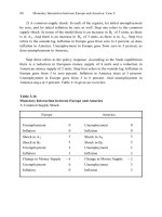
1) A demand shock. Let initial unemployment be zero, and let initial inflation
be zero as well. Step one refers to a decline in aggregate demand. In terms of the
model there is an increase in A of 2 units and a decline in B of equally 2 units.
Monetary and Fiscal Cooperation

29
Step two refers to the outside lag. Unemployment goes from zero to 2 percent.
And inflation goes from zero to – 2 percent. Step three refers to the policy
response. According to the model, a first solution is an increase in money supply
of 2 units and an increase in government purchases of zero units. Step four refers
to the outside lag. Unemployment goes from 2 to zero percent. And inflation
goes from – 2 to zero percent. Table 1.5 presents a synopsis.


As a result, given a demand shock, monetary and fiscal cooperation achieves
both zero inflation and zero unemployment. A second solution is an increase in
money supply of 1 unit and an increase in government purchases of equally 1
unit. A third solution is an increase in money supply of zero units and an increase
in government purchases of 2 units. And so on. The loss function under policy
cooperation is:


22
Lu=π + (6)

The initial loss is zero. The demand shock causes a loss of 8 units. Then policy
cooperation brings the loss down to zero again.


Table 1.5
Cooperation between Central Bank and Government
A Demand Shock


Unemployment 0 Inflation 0
Shock in A 2 Shock in B
− 2
Unemployment 2 Inflation
− 2
Change in Money Supply 2 Change in Govt Purchases 0
Unemployment 0 Inflation 0




2) A supply shock. Let initial unemployment and inflation be zero each. Step
one refers to the supply shock. In terms of the model there is an increase in B of
2. Some Numerical Examples

30
2 units and an increase in A of equally 2 units. Step two refers to the outside lag.
Inflation goes from zero to 2 percent. And unemployment goes from zero to 2
percent as well. Step three refers to the policy response. According to the model,
a first solution is to keep money supply and government purchases constant. Step
four refers to the outside lag. Obviously, inflation stays at 2 percent, and
unemployment stays at 2 percent as well. Table 1.6 gives an overview.

As a result, given a supply shock, monetary and fiscal cooperation is
ineffective. The initial loss is zero. The supply shock causes a loss of 8 units.
Then policy cooperation keeps the loss at 8 units.


Table 1.6
Cooperation between Central Bank and Government
A Supply Shock


Unemployment 0 Inflation 0
Shock in A 2 Shock in B 2
Unemployment 2 Inflation 2
Change in Money Supply 0 Change in Govt Purchases 0
Unemployment 2 Inflation 2




3) A mixed shock. Let initial unemployment and inflation be zero each. Step
one refers to the mixed shock. In terms of the model there is an increase in B of 4
units. Step two refers to the outside lag. Inflation goes from zero to 4 percent.
And unemployment stays at zero percent. Step three refers to the policy response.
According to the model, a first solution is a reduction in money supply of 2 units
and a reduction in government purchases of zero units. Step four refers to the
outside lag. Inflation goes from 4 to 2 percent. And unemployment goes from
zero to 2 percent. For a synopsis see Table 1.7.

As a result, given a mixed shock, monetary and fiscal cooperation lowers
inflation. On the other hand, it raises unemployment. A second solution is a
Monetary and Fiscal Cooperation

31
reduction in money supply of 1 unit and a reduction in government purchases of
equally 1 unit. A third solution is a reduction in money supply of zero units and a
reduction in government purchases of 2 units. And so on. The initial loss is zero.
The mixed shock causes a loss of 16 units. Then policy cooperation brings the
loss down to 8 units.


Table 1.7
Cooperation between Central Bank and Government
A Mixed Shock


Unemployment 0 Inflation 0
Shock in A 0 Shock in B 4
Unemployment 0 Inflation 4
Change in Money Supply

− 2
Change in Govt Purchases 0
Unemployment 2 Inflation 2



4) Summary. Given a demand shock, policy cooperation achieves both zero
inflation and zero unemployment. Given a supply shock, policy cooperation is
ineffective. Given a mixed shock, policy cooperation reduces the loss to a certain
extent.

5) Comparing policy interaction and policy cooperation. Under policy
interaction there is no Nash equilibrium. By contrast, policy cooperation can
reduce the loss caused by inflation and unemployment. Judging from this point of
view, policy cooperation seems to be superior to policy interaction.


2. Some Numerical Examples
Part Two


The Closed Economy


Presence of a Deficit Target

35
Chapter 1
Fiscal Policy


1. The Model



An increase in government purchases lowers unemployment. On the other
hand, it raises inflation. And what is more, it raises the structural deficit. The
targets of the government are zero unemployment and a zero structural deficit.

The model of unemployment, inflation, and the structural deficit can be
represented by a system of three equations:


AG
u
Y
−
=
(1)

BG
Y
+
π=
(2)

GT
s
Y
−
=

(3)

Here
u
denotes the rate of unemployment,
π
is the rate of inflation, s is the
structural deficit ratio, G is government purchases, T is tax revenue at full-
employment output,
GT−
is the structural deficit, A is some other factors
bearing on the rate of unemployment,
B is some other factors bearing on the rate
of inflation, and
Y is full-employment output. The endogenous variables are the
rate of unemployment, the rate of inflation, and the structural deficit ratio.

According to equation (1), the rate of unemployment is a positive function of
A and a negative function of government purchases. According to equation (2),
the rate of inflation is a positive function of B and a positive function of
government purchases. According to equation (3), the structural deficit ratio is a
positive function of government purchases.


M. Carlberg, Monetary and Fiscal Strategies in the World Economy, 35
DOI 10.1007/978-3-642-10476-3_6, © Springer-Verlag Berlin Heidelberg 2010

36
To simplify notation we assume that full-employment output is unity. On this
assumption, the model can be written as follows:



uAG=−
(4)

BGπ= +
(5)

sGT=−
(6)

A unit increase in government purchases lowers the rate of unemployment by 1
percentage point. On the other hand, it raises the rate of inflation by 1 percentage
point. And what is more, it raises the structural deficit ratio by 1 percentage
point. For instance, let initial unemployment be 2 percent, let initial inflation be 2
percent, and let the initial structural deficit be 2 percent as well. Now consider a
unit increase in government purchases. Then unemployment goes from 2 to 1
percent. On the other hand, inflation goes from 2 to 3 percent. And what is more,
the structural deficit goes from 2 to 3 percent as well.

The targets of the government are zero unemployment and a zero structural
deficit. The instrument of the government is government purchases. There are
two targets but only one instrument, so what is needed is a loss function. We
assume that the government has a quadratic loss function:


22
2
Lus=+
(7)


2
L is the loss to the government caused by unemployment and the structural
deficit. We assume equal weights in the loss function. The specific target of the
government is to minimize the loss, given the unemployment function and the
structural deficit function. Taking account of equations (4) and (6), the loss
function of the government can be written as follows:


22
2
L(AG)(GT)=− +−
(8)

Then the first-order condition for a minimum loss is:


2G A T=+
(9)

Fiscal Policy

37
Here G is the optimum level of government purchases. An increase in A requires
an increase in government purchases. And an increase in B requires no change in
government purchases. From equations (4) and (9) follows the optimum rate of
unemployment:


2u A T=−

(10)

From equations (5) and (9) follows the optimum rate of inflation:


2A2BTπ= + +
(11)

And from equations (6) and (9) follows the optimum structural deficit ratio:


2s A T=−
(12)

Unemployment is not zero. And the same holds for inflation and the structural
deficit.
1. The Model

38
2. Some Numerical Examples



For easy reference, the basic model is summarized here:


uAG=−
(1)

π BG=+

(2)

sGT=−
(3)

And the optimum level of government purchases is:


2G A T=+
(4)

It proves useful to study two distinct cases:
- a demand shock
- a supply shock.

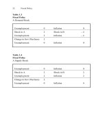
1) A demand shock. Let initial unemployment be zero, let initial inflation be
zero, and let the initial structural deficit be zero as well. Step one refers to a
decline in aggregate demand. In terms of the model there is an increase in A of 6
units and a decline in B of equally 6 units. Step two refers to the outside lag.
Unemployment goes from zero to 6 percent. Inflation goes from zero to – 6
percent. And the structural deficit stays at zero percent. Step three refers to the
policy response. What is needed, according to the model, is an increase in
government purchases of 3 units. Step four refers to the outside lag.
Unemployment goes from 6 to 3 percent. The structural deficit goes from zero to
3 percent. And inflation goes from – 6 to – 3 percent. Table 2.1 presents a
synopsis.

As a result, given a demand shock, fiscal policy lowers unemployment and
deflation. On the other hand, it raises the structural deficit. The loss function of
the government is:



22
2
Lus=+ (5)
Fiscal Policy

39

The initial loss is zero. The demand shock causes a loss of 36 units. Then fiscal
policy brings the loss down to 18 units.


Table 2.1
Fiscal Policy
A Demand Shock


Unemployment 0 Inflation 0
Structural Deficit 0
Shock in A 6 Shock in B
− 6
Unemployment 6 Inflation
− 6
Structural Deficit 0
Change in Govt Purchases 3
Unemployment 3 Inflation
− 3
Structural Deficit 3




2) A supply shock. Let initial unemployment be zero, let initial inflation be
zero, and let the initial structural deficit be zero as well. Step one refers to the
supply shock. In terms of the model there is an increase in B of 6 units and an
increase in A of equally 6 units. Step two refers to the outside lag. Inflation goes
from zero to 6 percent. Unemployment goes from zero to 6 percent as well. And
the structural deficit stays at zero percent. Step three refers to the policy
response. What is needed, according to the model, is an increase in government
purchases of 3 units. Step four refers to the outside lag. Unemployment goes
from 6 to 3 percent. The structural deficit goes from zero to 3 percent. And
inflation goes from 6 to 9 percent. Table 2.2 gives an overview.

As a result, given a supply shock, fiscal policy lowers unemployment. On the
other hand, it raises the structural deficit. And what is more, it raises inflation.
2. Some Numerical Examples

40
The initial loss is zero. The supply shock causes a loss of 36 units. Then fiscal
policy reduces the loss to 18 units.

3) Summary. Given a demand shock, fiscal policy can reduce the loss to a
certain extent. And the same is true of a supply shock.


Table 2.2
Fiscal Policy
A Supply Shock



Unemployment 0 Inflation 0
Structural Deficit 0
Shock in A 6 Shock in B 6
Unemployment 6 Inflation 6
Structural Deficit 0
Change in Govt Purchases 3
Unemployment 3 Inflation 9
Structural Deficit 3


Fiscal Policy

41
Chapter 2

1. The Model



An increase in money supply lowers unemployment. On the other hand, it
raises inflation. However, it has no effect on the structural deficit. Corres-
pondingly, an increase in government purchases lowers unemployment. On the
other hand, it raises inflation. And what is more, it raises the structural deficit.
The target of the central bank is zero inflation. By contrast, the targets of the
government are zero unemployment and a zero structural deficit.

The model of unemployment, inflation, and the structural deficit can be
characterized by a system of three equations:



uAMG=−− (1)

BMGπ= + + (2)

sGT=−
(3)

Here u denotes the rate of unemployment,
π
is the rate of inflation, s is the
structural deficit ratio, M is money supply, G is government purchases, T is tax
revenue at full-employment output,
GT
−
is the structural deficit, A is some
other factors bearing on the rate of unemployment, and B is some other factors
bearing on the rate of inflation. The endogenous variables are the rate of
unemployment, the rate of inflation, and the structural deficit ratio.

According to equation (1), the rate of unemployment is a positive function of
A, a negative function of money supply, and a negative function of government
purchases. According to equation (2), the rate of inflation is a positive function of
B, a positive function of money supply, and a positive function of government
purchases. According to equation (3), the structural deficit ratio is a positive
function of government purchases. A unit increase in money supply lowers the
rate of unemployment by 1 percentage point. On the other hand, it raises the rate
Monetary and Fiscal Interaction
M. Carlberg, Monetary and Fiscal Strategies in the World Economy, 41
DOI 10.1007/978-3-642-10476-3_7, © Springer-Verlag Berlin Heidelberg 2010


42
of inflation by 1 percentage point. However, it has no effect on the structural
deficit ratio. A unit increase in government purchases lowers the rate of
unemployment by 1 percentage point. On the other hand, it raises the rate of
inflation by 1 percentage point. And what is more, it raises the structural deficit
ratio by 1 percentage point.

The target of the central bank is zero inflation. The instrument of the central
bank is money supply. By equation (2), the reaction function of the central bank
is:


MBG=− − (4)

Suppose the government raises government purchases. Then, as a response, the
central bank lowers money supply.

The targets of the government are zero unemployment and a zero structural
deficit. The instrument of the government is government purchases. There are
two targets but only one instrument, so what is needed is a loss function. We
assume that the government has a quadratic loss function:


22
2
Lus=+ (5)

2
L is the loss to the government caused by unemployment and the structural
deficit. We assume equal weights in the loss function. The specific target of the

government is to minimize the loss, given the unemployment function and the
structural deficit function. Taking account of equations (1) and (3), the loss
function of the government can be written as follows:


22
2
L(AMG)(GT)=−− +− (6)

Then the first-order condition for a minimum loss gives the reaction function of
the government:


2G A T M=+− (7)

Suppose the central bank lowers money supply. Then, as a response, the
government raises government purchases.
Monetary and Fiscal Interaction

43

The Nash equilibrium is determined by the reaction functions of the central
bank and the government. The solution to this problem is as follows:


MA2BT=− − − (8)

GABT=++ (9)

Equations (8) and (9) show the Nash equilibrium of money supply and

government purchases. As a result there is a unique Nash equilibrium. An
increase in A causes a decline in money supply and an increase in government
purchases. And the same applies to an increase in B. A unit increase in A causes
a decline in money supply of 1 unit and an increase in government purchases of
equally 1 unit. A unit increase in B causes a decline in money supply of 2 units
and an increase in government purchases of 1 unit.

From equations (1), (8) and (9) follows the equilibrium rate of unemploy-
ment:


uAB=+ (10)

From equations (2), (8) and (9) follows the equilibrium rate of inflation:


0π= (11)

And from equations (3) and (9) follows the equilibrium structural deficit ratio:


sAB=+ (12)

Inflation is zero. By contrast, unemployment is not zero, nor is the structural
deficit.



1. The Model


44
2. Some Numerical Examples



For easy reference, the basic model is summarized here:


uAMG=−− (1)

BMGπ= + + (2)

sGT=− (3)

And the Nash equilibrium can be described by two equations:


MA2BT=− − − (4)

GABT=++ (5)

It proves useful to study two distinct cases:
-
a demand shock
-
a supply shock.

1) A demand shock. Let initial unemployment be zero, let initial inflation be
zero, and let the initial structural deficit be zero as well. Step one refers to a
decline in aggregate demand. In terms of the model there is an increase in A of 2

units and a decline in B of equally 2 units. Step two refers to the outside lag.
Unemployment goes from zero to 2 percent. Inflation goes from zero to – 2
percent. And the structural deficit stays at zero percent. Step three refers to the
policy response. According to the Nash equilibrium there is an increase in money
supply of 2 units and an increase in government purchases of zero units. Step
four refers to the outside lag. Unemployment goes from 2 to zero percent.
Inflation goes from – 2 to zero percent. And the structural deficit stays at zero
percent. Table 2.3 presents a synopsis.

As a result, given a demand shock, monetary and fiscal interaction achieves
zero inflation, zero unemployment, and a zero structural deficit. The loss
functions of the central bank and the government are respectively:

Monetary and Fiscal Interaction

45
2
1
L =π (6)
22
2
Lus=+ (7)

The initial loss of the central bank is zero, as is the initial loss of the government.
The demand shock causes a loss to the central bank of 4 units and a loss to the
government of equally 4 units. Then policy interaction reduces the loss of the
central bank to zero. Correspondingly, policy interaction reduces the loss of the
government to zero.



Table 2.3
Interaction between Central Bank and Government
A Demand Shock


Unemployment 0 Inflation 0
Structural Deficit 0
Shock in A 2 Shock in B
− 2
Unemployment 2 Inflation
− 2
Structural Deficit 0
Change in Money Supply 2 Change in Govt Purchases 0
Unemployment 0 Inflation 0
Structural Deficit 0



2) A supply shock. Let initial unemployment be zero, let initial inflation be
zero, and let the initial structural deficit be zero as well. Step one refers to the
supply shock. In terms of the model there is an increase in B of 2 units and an
increase in A of equally 2 units. Step two refers to the outside lag. Inflation goes
from zero to 2 percent. Unemployment goes from zero to 2 percent as well. And
the structural deficit stays at zero percent. Step three refers to the policy
response. According to the Nash equilibrium there is a reduction in money
supply of 6 units and an increase in government purchases of 4 units. Step four
refers to the outside lag. Inflation goes from 2 to zero percent. Unemployment
2. Some Numerical Examples

46

goes from 2 to 4 percent. And the structural deficit goes from zero to 4 percent.
Table 2.4 gives an overview.

As a result, given a supply shock, monetary and fiscal interaction achieves
zero inflation. On the other hand, it raises unemployment and the structural
deficit. The initial loss of each policy maker is zero. The supply shock causes a
loss to the central bank of 4 units and a loss to the government of equally 4 units.
Then policy interaction reduces the loss of the central bank from 4 to zero units.
However, it increases the loss of the government from 4 to 32 units. To sum up,
policy interaction increases the total loss from 8 to 32 units.

3) Summary. Given a demand shock, policy interaction achieves zero
inflation, zero unemployment, and a zero structural deficit. Given a supply shock,
policy interaction achieves zero inflation. On the other hand, it raises
unemployment and the structural deficit.


Table 2.4
Interaction between Central Bank and Government
A Supply Shock


Unemployment 0 Inflation 0
Structural Deficit 0
Shock in A 2 Shock in B 2
Unemployment 2 Inflation 2
Structural Deficit 0
Change in Money Supply
− 6
Change in Govt Purchases 4

Unemployment 4 Inflation 0
Structural Deficit 4



Monetary and Fiscal Interaction

47
Chapter 3
Monetary and Fiscal Cooperation

1. The Model



The model of unemployment, inflation, and the structural deficit can be
represented by a system of three equations:


uAMG=−−
(1)

BMGπ= + +
(2)

sGT=−
(3)

The policy makers are the central bank and the government. The targets of
policy cooperation are zero inflation, zero unemployment, and a zero structural

deficit. The instruments of policy cooperation are money supply and government
purchases. There are three targets but only two instruments, so what is needed is
a loss function. We assume that the policy makers agree on a common loss
function:


222
Lus=π + + (4)

L is the loss caused by inflation, unemployment, and the structural deficit. We
assume equal weights in the loss function. The specific target of policy
cooperation is to minimize the loss, given the inflation function, the
unemployment function, and the structural deficit function. Taking account of
equations (1), (2) and (3), the loss function under policy cooperation can be
written as follows:


222
L(BMG) (AMG) (GT)=++ +−− +− (5)

Then the first-order conditions for a minimum loss are:


2M A B 2G=−−
(6)

M. Carlberg, Monetary and Fiscal Strategies in the World Economy, 47
DOI 10.1007/978-3-642-10476-3_8, © Springer-Verlag Berlin Heidelberg 2010

48


3G A T B 2M=+−−
(7)

Equation (6) shows the first-order condition with respect to money supply. And
equation (7) shows the first-order condition with respect to government
purchases.

The cooperative equilibrium is determined by the first-order conditions for a
minimum loss. The solution to this problem is as follows:


2M A B 2T=−− (8)

GT=
(9)

Equations (8) and (9) show the cooperative equilibrium of money supply and
government purchases. As a result there is a unique cooperative equilibrium. An
increase in A causes an increase in money supply. And an increase in B causes a
decline in money supply. A unit increase in A causes an increase in money
supply of 0.5 units. And a unit increase in B causes a decline in money supply of
equally 0.5 units.

From equations (1), (8) and (9) follows the optimum rate of unemployment:


2u A B=+
(10)


From equations (2), (8) and (9) follows the optimum rate of inflation:


2ABπ= +
(11)

And from equations (3) and (9) follows the optimum structural deficit ratio:


s0=
(12)

The structural deficit is zero. By contrast, unemployment and inflation are not
zero.
Monetary and Fiscal Cooperation