Air Quality318

When Brager studied office buildings in San Francisco during the winter, he revealed that
the PMV was found to be lower (colder) than the obtained thermal sensation. That defined a
neutral temperature of 24.8ºC, which was 2.4ºC above the estimated value. After considering
various UK offices with mechanical ventilation, it was demonstrated that the PMV differed
by 0.5 points with the thermal sensation, which is equivalent to 1.5ºC differences.
In Australia, Dear and Auliciems (1985), found a difference of 0.5–3.2º C between the neutral
temperatures, estimated by surveys and determined by the PMV model of Fanger.
Subsequently, Dear conducted a study in 12 Australian office buildings; it was defined that
a temperature difference, between neutral temperatures proposed by surveys and PMV, was
determined to about 1ºC. Dear et al. extended their studies to those made by Brager. They
returned to analyze and correct the data by the seat isolation. Again, discrepancies were
found between the neutral temperature, based on the value obtained through surveys, and
the value predicted by the equations. As a result, it seems that for real conditions, the
thermal sensation of neutrality is in line with a deviation of the order of 0.2–3.3ºC and an
average of 1.4ºC of the thermal neutrality conditions. The error was attributed to a PMV
erroneous definition of the metabolic activity and the index of clo, or unable to take into
account the isolation of the seat.
The Institute for Environmental Research of the State University of Kansas, under ASHRAE
contract, has conducted extensive research on the subject of thermal comfort in sedentary
regime. The purpose of this investigation was to obtain a model to express the PMV in terms
of parameters easily sampled in an environment. As a result, an investigation of 1,600
school-age students revealed statistics correlations between the level of comfort,
temperature, humidity, sex and exposure duration. Groups consisting of 5 men and 5
women were exposed to a range of temperatures between 15.6 and 36.7ºC, with increases of
1.1ºC at 8 different relative humidifies of 15, 25, 34, 45, 55, 65, 75 and 85% and for air speeds
of lower than 0.17 m/s. During a study period of 3 hours and in intervals of half hours,
subjects reported their thermal sensations on a ballot paper with 7 categories ranging
between –3 and 3 (Table 4). These categories show a thermal sensation that varies between
cold and warm, passing 0 that indicates thermal neutrality. The results have yielded to an

expression of the form (Equation 6).


cpbtaPMV
v

(6)

Time/sex

A

B

C

1 hour/
m
an

0.220

0.233

5.673

Woman

0.272


0.248

7.245

Both

0.245

0.248

6.475

2 hours/
m
an

0.221

0.270

6.024

Woman

0.283

0.210

7.694


Both 0.252 0.240 6.859
3 hours/
m
an

0.212

0.293

5.949

Woman

0.275

0.255

8.620

Both

0.243

0.278

6.802

Table 5. The coefficients a, b and c are a function of spent time and the sex of the subject.



By using this equation and taking into account sex and exposure time to the indoor
environment, it should be used as constants (Table 5).
With these criteria, a comfort zone is, on average, close to conditions of 26ºC and 50%
relative humidity. The study subjects have undergone a sedentary metabolic activity,
dressed in normal clothes and with a thermal resistance of approximately 0.6 clo. Its
exposure to the indoor ambiences was for 3 hours.

4. Results on Local Thermal Comfort Models
For an indoor air quality study, there are a number of empirical equations used by some
authors over the last few years (Simonson et al., 2001). Indices, such as the percentage of
dissatisfaction with local thermal comfort, thermal sensation and indoor air acceptability,
are determined in terms of some simple parameter measures, such as dry bulb temperature
and relative humidity. For instance, the humidity ratio and relative humidity are the most
important parameters to compare the effect of moisture in the environment, whereas
temperature and enthalpy reflect the thermal energy of each psychometric process.
Simonson revealed that moisture had a small effect on thermal comfort, but a lot more on
the local thermal comfort. The current regulations (ISO 7730, ASHRAE and DIN 1946) do
not coincide with the exact value of moisture in the environment for some conditions, but
concludes that a very high or very low relative humidity worsens comfort conditions.
The agreement chosen by ANSI/ASHRAE and ISO 7730 to establish the comfort boundary
conditions was about 10% of dissatisfaction. Other authors believe that the local thermal
comfort is primarily a function of not only the thermal gradient at different altitudes and air
speeds, but may be also owing to the presence of sweat on the skin or inadequate mucous
membrane refrigeration. To meet the local thermal comfort produced by the interior air
conditions, Toftum et al. (1998a, b) studied the response of 38 individuals who were
provided with clean air in a closed environment. The air temperature conditions ranged
between 20 and 29ºC and the humidity ratio between 6 and 19 g/kg, as from 20ºC and 45%
RH to 29ºC and 70% RH. Individuals assessed the ambient air with three or four puffs, and
thus the equation for the percentage of local dissatisfaction was developed (Equation 7).
ASHRAE recommends keeping the percentage of local dissatisfaction below 15% and the

percentage of general thermal comfort dissatisfaction below 10. This PD tends to decrease
when the temperature decreases and, as a result, limited conditions can be employed to
define the optimal conditions for energy saving in the air conditioning system.

)01.05.42(14.0)30(18.058.3(
1
100
v
pt
e
PD



(7)

Where:
p
v
is the partial vapour pressure (Pa)

4.1. Air velocity models
Air velocity affects sensible heat dissipated by convection and latent heat dissipated by
evaporation, because both the convection coefficient and the amount of evaporated water
per unit of time depend on it; therefore, the restful feeling becomes affected by air drafts.
A review of general and local thermal comfort models for controlling indoor ambiences 319

When Brager studied office buildings in San Francisco during the winter, he revealed that
the PMV was found to be lower (colder) than the obtained thermal sensation. That defined a
neutral temperature of 24.8ºC, which was 2.4ºC above the estimated value. After considering

various UK offices with mechanical ventilation, it was demonstrated that the PMV differed
by 0.5 points with the thermal sensation, which is equivalent to 1.5ºC differences.
In Australia, Dear and Auliciems (1985), found a difference of 0.5–3.2º C between the neutral
temperatures, estimated by surveys and determined by the PMV model of Fanger.
Subsequently, Dear conducted a study in 12 Australian office buildings; it was defined that
a temperature difference, between neutral temperatures proposed by surveys and PMV, was
determined to about 1ºC. Dear et al. extended their studies to those made by Brager. They
returned to analyze and correct the data by the seat isolation. Again, discrepancies were
found between the neutral temperature, based on the value obtained through surveys, and
the value predicted by the equations. As a result, it seems that for real conditions, the
thermal sensation of neutrality is in line with a deviation of the order of 0.2–3.3ºC and an
average of 1.4ºC of the thermal neutrality conditions. The error was attributed to a PMV
erroneous definition of the metabolic activity and the index of clo, or unable to take into
account the isolation of the seat.
The Institute for Environmental Research of the State University of Kansas, under ASHRAE
contract, has conducted extensive research on the subject of thermal comfort in sedentary
regime. The purpose of this investigation was to obtain a model to express the PMV in terms
of parameters easily sampled in an environment. As a result, an investigation of 1,600
school-age students revealed statistics correlations between the level of comfort,
temperature, humidity, sex and exposure duration. Groups consisting of 5 men and 5
women were exposed to a range of temperatures between 15.6 and 36.7ºC, with increases of
1.1ºC at 8 different relative humidifies of 15, 25, 34, 45, 55, 65, 75 and 85% and for air speeds
of lower than 0.17 m/s. During a study period of 3 hours and in intervals of half hours,
subjects reported their thermal sensations on a ballot paper with 7 categories ranging
between –3 and 3 (Table 4). These categories show a thermal sensation that varies between
cold and warm, passing 0 that indicates thermal neutrality. The results have yielded to an
expression of the form (Equation 6).


cpbtaPMV

v





(6)

Time/sex

A

B

C

1 hour/
m
an

0.220

0.233

5.673

Woman

0.272


0.248

7.245

Both

0.245

0.248

6.475

2 hours/
m
an

0.221

0.270

6.024

Woman

0.283

0.210

7.694


Both

0.252

0.240

6.859

3 hours/
m
an

0.212

0.293

5.949

Woman

0.275

0.255

8.620

Both

0.243


0.278

6.802

Table 5. The coefficients a, b and c are a function of spent time and the sex of the subject.


By using this equation and taking into account sex and exposure time to the indoor
environment, it should be used as constants (Table 5).
With these criteria, a comfort zone is, on average, close to conditions of 26ºC and 50%
relative humidity. The study subjects have undergone a sedentary metabolic activity,
dressed in normal clothes and with a thermal resistance of approximately 0.6 clo. Its
exposure to the indoor ambiences was for 3 hours.

4. Results on Local Thermal Comfort Models
For an indoor air quality study, there are a number of empirical equations used by some
authors over the last few years (Simonson et al., 2001). Indices, such as the percentage of
dissatisfaction with local thermal comfort, thermal sensation and indoor air acceptability,
are determined in terms of some simple parameter measures, such as dry bulb temperature
and relative humidity. For instance, the humidity ratio and relative humidity are the most
important parameters to compare the effect of moisture in the environment, whereas
temperature and enthalpy reflect the thermal energy of each psychometric process.
Simonson revealed that moisture had a small effect on thermal comfort, but a lot more on
the local thermal comfort. The current regulations (ISO 7730, ASHRAE and DIN 1946) do
not coincide with the exact value of moisture in the environment for some conditions, but
concludes that a very high or very low relative humidity worsens comfort conditions.
The agreement chosen by ANSI/ASHRAE and ISO 7730 to establish the comfort boundary
conditions was about 10% of dissatisfaction. Other authors believe that the local thermal
comfort is primarily a function of not only the thermal gradient at different altitudes and air
speeds, but may be also owing to the presence of sweat on the skin or inadequate mucous

membrane refrigeration. To meet the local thermal comfort produced by the interior air
conditions, Toftum et al. (1998a, b) studied the response of 38 individuals who were
provided with clean air in a closed environment. The air temperature conditions ranged
between 20 and 29ºC and the humidity ratio between 6 and 19 g/kg, as from 20ºC and 45%
RH to 29ºC and 70% RH. Individuals assessed the ambient air with three or four puffs, and
thus the equation for the percentage of local dissatisfaction was developed (Equation 7).
ASHRAE recommends keeping the percentage of local dissatisfaction below 15% and the
percentage of general thermal comfort dissatisfaction below 10. This PD tends to decrease
when the temperature decreases and, as a result, limited conditions can be employed to
define the optimal conditions for energy saving in the air conditioning system.

)01.05.42(14.0)30(18.058.3(
1
100
v
pt
e
PD



(7)

Where:
p
v
is the partial vapour pressure (Pa)

4.1. Air velocity models
Air velocity affects sensible heat dissipated by convection and latent heat dissipated by

evaporation, because both the convection coefficient and the amount of evaporated water
per unit of time depend on it; therefore, the restful feeling becomes affected by air drafts.
Air Quality320

Aiming towards energy saving in summer, the ambient air temperature can be kept slightly
higher than the optimum and achieve a more pleasant feeling by increasing air velocity. The
maximum acceptable air speed is 0.9 m/s.
In winter, the air circulation causes a cold feeling and to keep air temperature above that
needed to avoid a feeling of discomfort, with its corresponding energy consumption. In
winter, considering that the dry air temperature tends to be in the low band of comfort, air
conditions in inhabited areas must be carefully studied, in order to maintain the conditions
of wellbeing without wasting energy. It is recommended that the winter air velocity in the
inhabited zone should be lower than 0.15 m/s. Localized draft problems are more common
in indoor environments, vehicles and aircraft, with air conditioning. Even without a speed-
sensitive air, there may be dissatisfaction owing to excessive cooling somewhere in the
body.
In principle, there is sensitivity to currents on the nude parts of the body; therefore, only
noticeable current flows on the face, hands and lower legs. The amount of heat lost through
the skin because of the flow depends on the average speed of air, temperature and
turbulence. Owing to the behaviour of the cold sensors on the skin, the degree of discomfort
depends not only on the loss of local heat, but also on the influence in temperature
fluctuations. For equal thermal losses, there is a greater sense of dissatisfaction with high
turbulence in the air flow.
Some studies exhibit the types of fluctuations that cause greater dissatisfaction. These have
been obtained from groups of individuals subjected to various air speed frequencies. The
oscillations with a frequency of 0.5 Hz are the most uncomfortable, whereas oscillations
with a higher frequency of 2 Hz produce less sensitive effects.
According to the ISO 7730:2005, drafts produce an unwanted local cooling in the human
body. The flow risk can be expressed as the percentage of annoyed individuals and
calculated (Equation 8).

The draft risk model is based on studies of 150 subjects exposed to air temperatures between
20 and 26ºC, with average air speed between 0.05 and 0.4 m/s and turbulence intensities
from 0 to 70%. The model is also applicable to low densities of people, with sedentary
activity and a neutral thermal sensation over the full body.
The draft risk is lower for non-sedentary activities and for people with neutral thermal
sensation conditions. Fig. 7 reveals the relationship between air speed, temperature and the
degree of turbulence, for a percentage of dissatisfaction of 10 or 20%. The different curves
refer to a percentage of turbulence from 10 to 80.

)14.337.0()05.0)(34(
62.0

u
vTvtDR
(8)

Where:
v is the air velocity (m/s)
t is the air temperature (ºC)
Tu is turbulence intensity (%)


DR=15%
0
0.1
0.2
0.3
0.4
0.5
18 20 22 24 26 28 30

Air Temperature (ºC)
Mean air velocity (m/s)
Tu=0 Tu=10 Tu=20 Tu=80

Fig. 7. Average air velocity, depending on temperature and the degree of turbulence thermal
environments, for type A, B and C.

4.2. Asymmetric thermal radiation
A person located in front of an intense external heat source, in cold weather, may notice
after a certain period of time some dissatisfaction. The reason is the excessive warm front
and high cooling on the other side. This uncomfortable situation could be remedied with
frequent changes in position to achieve a more uniform heating. This example reveals the
uncomfortable conditions owing to a non-uniform radiant heat effect.
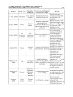
To evaluate the non-uniform thermal radiation, the asymmetric thermal radiation parameter
(
r
t ) is used. This parameter is defined on the basis of the difference between the flat
radiation temperature (
pr
t
) of the two opposite sides of a small plane element. The
experiences of individuals exposed to variations in asymmetrical radiant temperature, such
as the conditions caused by warm roofs and cold windows, produce the greatest impact of
dissatisfaction. During earlier experiences, the surface of the enclosure and air temperature
was preserved.

Percentage of dissatisfied
1
10
100

5 10 15 20 25 30
Asymmetrical Radiant Temperature (ºC)
PD
Hot Ceiling Cold Wall Cold Ceiling Hot Wall

Fig. 8. Percentage of dissatisfied as a function of asymmetrical radiant temperature,
produced by a roof or wall cold or hot.
A review of general and local thermal comfort models for controlling indoor ambiences 321

Aiming towards energy saving in summer, the ambient air temperature can be kept slightly
higher than the optimum and achieve a more pleasant feeling by increasing air velocity. The
maximum acceptable air speed is 0.9 m/s.
In winter, the air circulation causes a cold feeling and to keep air temperature above that
needed to avoid a feeling of discomfort, with its corresponding energy consumption. In
winter, considering that the dry air temperature tends to be in the low band of comfort, air
conditions in inhabited areas must be carefully studied, in order to maintain the conditions
of wellbeing without wasting energy. It is recommended that the winter air velocity in the
inhabited zone should be lower than 0.15 m/s. Localized draft problems are more common
in indoor environments, vehicles and aircraft, with air conditioning. Even without a speed-
sensitive air, there may be dissatisfaction owing to excessive cooling somewhere in the
body.
In principle, there is sensitivity to currents on the nude parts of the body; therefore, only
noticeable current flows on the face, hands and lower legs. The amount of heat lost through
the skin because of the flow depends on the average speed of air, temperature and
turbulence. Owing to the behaviour of the cold sensors on the skin, the degree of discomfort
depends not only on the loss of local heat, but also on the influence in temperature
fluctuations. For equal thermal losses, there is a greater sense of dissatisfaction with high
turbulence in the air flow.
Some studies exhibit the types of fluctuations that cause greater dissatisfaction. These have
been obtained from groups of individuals subjected to various air speed frequencies. The

oscillations with a frequency of 0.5 Hz are the most uncomfortable, whereas oscillations
with a higher frequency of 2 Hz produce less sensitive effects.
According to the ISO 7730:2005, drafts produce an unwanted local cooling in the human
body. The flow risk can be expressed as the percentage of annoyed individuals and
calculated (Equation 8).
The draft risk model is based on studies of 150 subjects exposed to air temperatures between
20 and 26ºC, with average air speed between 0.05 and 0.4 m/s and turbulence intensities
from 0 to 70%. The model is also applicable to low densities of people, with sedentary
activity and a neutral thermal sensation over the full body.
The draft risk is lower for non-sedentary activities and for people with neutral thermal
sensation conditions. Fig. 7 reveals the relationship between air speed, temperature and the
degree of turbulence, for a percentage of dissatisfaction of 10 or 20%. The different curves
refer to a percentage of turbulence from 10 to 80.

)14.337.0()05.0)(34(
62.0

u
vTvtDR
(8)

Where:
v is the air velocity (m/s)
t is the air temperature (ºC)
Tu is turbulence intensity (%)


DR=15%
0
0.1

0.2
0.3
0.4
0.5
18 20 22 24 26 28 30
Air Temperature (ºC)
Mean air velocity (m/s)
Tu=0 Tu=10 Tu=20 Tu=80

Fig. 7. Average air velocity, depending on temperature and the degree of turbulence thermal
environments, for type A, B and C.

4.2. Asymmetric thermal radiation
A person located in front of an intense external heat source, in cold weather, may notice
after a certain period of time some dissatisfaction. The reason is the excessive warm front
and high cooling on the other side. This uncomfortable situation could be remedied with
frequent changes in position to achieve a more uniform heating. This example reveals the
uncomfortable conditions owing to a non-uniform radiant heat effect.
To evaluate the non-uniform thermal radiation, the asymmetric thermal radiation parameter
(
r
t ) is used. This parameter is defined on the basis of the difference between the flat
radiation temperature (
pr
t
) of the two opposite sides of a small plane element. The
experiences of individuals exposed to variations in asymmetrical radiant temperature, such
as the conditions caused by warm roofs and cold windows, produce the greatest impact of
dissatisfaction. During earlier experiences, the surface of the enclosure and air temperature
was preserved.


Percentage of dissatisfied
1
10
100
5 10 15 20 25 30
Asymmetrical Radiant Temperature (ºC)
PD
Hot Ceiling Cold Wall Cold Ceiling Hot Wall

Fig. 8. Percentage of dissatisfied as a function of asymmetrical radiant temperature,
produced by a roof or wall cold or hot.
Air Quality322

The Parameter can be obtained by two methods: the first is based on the measure in two
opposite directions, using a transducer to capture radiation that affects a small plane from
the corresponding hemisphere. The second is to obtain temperature measurements from all
surfaces of the surroundings and calculating the
pr
t
.
Equations 9, 10, 11 and 12 show the employed models for each case. Finally, the curves
obtained are reflected in Fig. 8.

Hot ceiling (
Ct
pr
º23
)
5.5

)174.084.2exp(1
100



pr
t
PD
(9)

Cold wall (
Ct
pr
º15
)
)345.061.6exp(1
100
pr
t
PD


(10)

Cold ceiling (
Ct
pr
º15
)
)50.093.9exp(1

100
pr
t
PD


(11)

Hot wall (
Ct
pr
º35
)
5.3
)052.072.3exp(1
100



pr
t
PD
(12)

Where:
pr
t
is the flat radiation temperature (ºC).

4.3. Vertical temperature difference

In general, there is an unsatisfied sensation with heat around the head and cold around the
feet, regardless of whether the cause is convection or radiation. We can express the vertical
temperature difference of the air existing at the ankle and neck height, respectively.
Experiments on people’s neutral thermal conditions have been conducted.
Based on these results, a temperature difference between head and feet of 3ºC produces a
dissatisfaction of 5%. The curve obtained is reflected in Fig. 9. For a person in a sedentary
activity, ISO 7730 is the acceptable value of 3ºC. The corresponding model is revealed in
Equation 13.

)856.076.5exp(1
100
t
PD


(13)

Percentage of dissatisfied
1
10
100
0 2 4 6 8 10
Vertical Temperature Difference (ºC)
PD

Fig. 9. Percentage of dissatisfied, depending on the vertical temperature difference.

4.4. Soil temperature
Direct contact between the feet and ground may cause local dissatisfaction, owing to a
temperature which is either too high or low. Heat losses are dependent on other parameters,

such as conductivity, heat capacity of the ground material and insulation capacity of the
entire foot–footwear. ISO 7730 standard provides levels of comfort in sedentary activities for
a 10% dissatisfied.
This leads to acceptable ground temperatures of between 19 and 29ºC. Studies have
designated obtaining the curve (Fig. 10), and Equation 14 reflects the model of the
percentage of dissatisfaction for different floor temperatures.

)0025.0118.0387.1exp(94100
2
ff
ttPD 
(14)
Where:
t
f
is the floor temperature (ºC).

Percentage of dissatisfied
1
10
100
5 15 25 35
Floor Temperature (ºC)
PD

Fig. 10. Percentage of dissatisfied, depending on the temperature of the floor.
A review of general and local thermal comfort models for controlling indoor ambiences 323

The Parameter can be obtained by two methods: the first is based on the measure in two
opposite directions, using a transducer to capture radiation that affects a small plane from

the corresponding hemisphere. The second is to obtain temperature measurements from all
surfaces of the surroundings and calculating the
pr
t

.
Equations 9, 10, 11 and 12 show the employed models for each case. Finally, the curves
obtained are reflected in Fig. 8.

Hot ceiling (
Ct
pr
º23


)
5.5
)174.084.2exp(1
100



pr
t
PD
(9)

Cold wall (
Ct
pr

º15
)
)345.061.6exp(1
100
pr
t
PD


(10)

Cold ceiling (
Ct
pr
º15


)
)50.093.9exp(1
100
pr
t
PD


(11)

Hot wall (
Ct
pr

º35
)
5.3
)052.072.3exp(1
100



pr
t
PD
(12)

Where:
pr
t
is the flat radiation temperature (ºC).

4.3. Vertical temperature difference
In general, there is an unsatisfied sensation with heat around the head and cold around the
feet, regardless of whether the cause is convection or radiation. We can express the vertical
temperature difference of the air existing at the ankle and neck height, respectively.
Experiments on people’s neutral thermal conditions have been conducted.
Based on these results, a temperature difference between head and feet of 3ºC produces a
dissatisfaction of 5%. The curve obtained is reflected in Fig. 9. For a person in a sedentary
activity, ISO 7730 is the acceptable value of 3ºC. The corresponding model is revealed in
Equation 13.

)856.076.5exp(1
100

t
PD


(13)

Percentage of dissatisfied
1
10
100
0 2 4 6 8 10
Vertical Temperature Difference (ºC)
PD

Fig. 9. Percentage of dissatisfied, depending on the vertical temperature difference.

4.4. Soil temperature
Direct contact between the feet and ground may cause local dissatisfaction, owing to a
temperature which is either too high or low. Heat losses are dependent on other parameters,
such as conductivity, heat capacity of the ground material and insulation capacity of the
entire foot–footwear. ISO 7730 standard provides levels of comfort in sedentary activities for
a 10% dissatisfied.
This leads to acceptable ground temperatures of between 19 and 29ºC. Studies have
designated obtaining the curve (Fig. 10), and Equation 14 reflects the model of the
percentage of dissatisfaction for different floor temperatures.

)0025.0118.0387.1exp(94100
2
ff
ttPD 

(14)
Where:
t
f
is the floor temperature (ºC).

Percentage of dissatisfied
1
10
100
5 15 25 35
Floor Temperature (ºC)
PD

Fig. 10. Percentage of dissatisfied, depending on the temperature of the floor.
Air Quality324

5. Conclusions and Future Research Works
Given the varied activities of international involvement in indoor environments, it was
necessary for an intense research report about thermal comfort models, based on results of
scientific research and actual ISO and ASHRAE Standards. From this research, it was
concluded that, apart from the thermal comfort models, there are many more theoretical
models, both deterministic and empirical. As a result, some empirical models (Equation 15)
present an interesting application to building design and/or environmental engineering
owing to its easy resolution. Furthermore, these models present a nearly similar prediction
of thermal comfort than Fanger’s model, if they are applied considering its respective
conditions of special interest for engineering application. Regardless, Fanger’s thermal
comfort model presents an in-depth analysis that relates variables that act in the thermal
sensation. As a result, this model is the principal tool to be employed as reference for future
research (Orosa et al., 2009a, b) about indoor parameters on thermal comfort and indoor air

quality.
cpbtaPMV
v

(15)

However, different parameters can alter general thermal comfort in localized zones of the
indoor environment, such as air velocity models, asymmetric thermal radiation, vertical
temperature difference, soil temperature and humidity conditions.
All these variables are related with the local thermal discomfort by the percentage of
dissatisfied that are expected to be found in this environment (PD). The result of the effect of
relative humidity on local thermal comfort, in particular, is of special interest (Equation 16).

)01.05.42(14.0)30(18.058.3(
1
100
v
pt
e
PD



(16)

Finally, an important conclusion for this review is that it is possible to save energy if you
lower the number of air changes, temperature and relative humidity (Orosa et al., 2008a, b,
2009c, d). These discussions, to maintain the PD with the corresponding energy savings, are
ongoing. Cold, very dry air with high pollution causes the same number of dissatisfaction
than clean, mild and more humid air. Of interest is that if there is a slight drop in

temperature and relative humidity, pollutants emitted by each of the materials (Fang, 1996)
will be reduced. However, field tests are recommended by the researchers, so that they can
perform characterization of environments according to their varying temperature and
relative humidity. This may start the validation of models that simulate these processes by
computer and implement HVAC systems to reach better comfort conditions and, at the
same time, other objectives, such as energy saving, materials conservancy or work risk
prevention in industrial ambiences (Orosa et al., 2008c).

6. Acknowledgements
I thank the University of A Coruña for their sponsorship of the project 5230252906.541A.64902.


7. References
ASHRAE 55-2004. (2004). Thermal Environmental Conditions for Human Occupancy.
ASHRAE Standard.
Berglund, L.; Cain, W.S. (1989). Perceived air quality and the thermal environment. In:
Proceedings of IAQ ’89: The Human Equation: Health and Comfort, San Diego, pp. 93–
99.
Cain, W.S.; Leaderer, B.P.; Isseroff, R.; Berglund, L.G.; Huey, R.J.; Lipsitt, E.D.; Perlman, D.
(1983). Ventilation requirements in buildings– I. Control of occupancy odour and
tobacco smoke odour,
Atmospheric Environment, 17, pp.1183–1197.
Cain, WS. (1974). Perception of odor intensity and the time-course of olfactory adaptatio.
ASHRAE Trans 80, pp.53–75.
Charles, K.E. (2003). Fanger’s Thermal Comfort and Draught Models. IRC-RR-162.
Http://irc.nrc-cnrc.gc.ca/ircpubs. (Accessed July 2009)
Fanger, P.O.; (1970). Thermal comfort. Analysis and applications in environmental
engineering. McGrawHill. ISBN:0-07-019915-9
Fang, L.; Clausen, G.; Fanger, P.O. (1998). Impact of Temperature and Humidity on
Perception of Indoor Air Quality During Immediate and Longer Whole-Body

Exposures.
Indoor Air. Vol. 8, Issue 4. pp.276-284.
Fiala, D.; Lomas, K.J.; Stohrer, M. (2001). Computer prediction of human thermoregulatory
and temperature responses to a wide range of environmental conditions.
Int. J.
Biometeorol. 45, 143-159.
Gunnarsen, L.; Fanger, P.O. (1992). Adaptation to indoor air pollution.
Environment
International
. 18, pp. 43–54.
ISO 7730:2005. (2005). Ergonomics of the thermal environment Analytical determination
and interpretation of thermal comfort using calculation of the PMV and PPD
indices and local thermal comfort criteria.
ISO 7726:2002. (2002). Ergonomics of the thermal environment - Instruments for measuring
physical quantities.
Knudsen, H.N.; Kjaer, U.D.; Nielsen, P.A. (1996). Characterisation of emissions from
building products: long term sensory evaluation, the impact of concentration and
air velocity. In:
Proceedings of Indoor Air ’96, Nagoya. International Conference on
Indoor Air Quality and Climate, Vol. 3, pp. 551–556.
McNall, Jr; P.E., Jaax; J., Rohles, F. H.; Nevins, R. G.; Springer, W. (1967). Thermal comfort
(and thermally neutral) conditions for three levels of activity.
ASHRAE Transactions,
73.
Nevins, R.G.; Rohles, F. H.; Springer, W.; Feyerherm, A. M. (1966). A temperature-humidity
chart for thermal comfort of seated persons.
ASHRAE Transactions, 72(1), 283-295.
Molina M. (2000). Impacto de la temperatura y la humedad sobre la salud y el confort
térmico, climatización de ambientes interiores (Tesis doctoral) . Universidad de A
Coruña.

Orosa, J.A.; García-Bustelo, E. J. (2009) (a) Ashrae Standard Application in Humid Climate
Ambiences”.
European Journal of Scientific Research. 27 , 1, pp.128-139.
Orosa, J.A.; Carpente, T. (2009) (b). Thermal Inertia Effect in Old Buildings.
European Journal
of Scientific Research. .27 ,2, pp.228-233.
Orosa, J.A.; Oliveira, A.C. (2009) (c). Energy saving with passive climate control methods in
Spanish office buildings.
Energy and Buildings, 41, 8, pp. 823-828.
A review of general and local thermal comfort models for controlling indoor ambiences 325

5. Conclusions and Future Research Works
Given the varied activities of international involvement in indoor environments, it was
necessary for an intense research report about thermal comfort models, based on results of
scientific research and actual ISO and ASHRAE Standards. From this research, it was
concluded that, apart from the thermal comfort models, there are many more theoretical
models, both deterministic and empirical. As a result, some empirical models (Equation 15)
present an interesting application to building design and/or environmental engineering
owing to its easy resolution. Furthermore, these models present a nearly similar prediction
of thermal comfort than Fanger’s model, if they are applied considering its respective
conditions of special interest for engineering application. Regardless, Fanger’s thermal
comfort model presents an in-depth analysis that relates variables that act in the thermal
sensation. As a result, this model is the principal tool to be employed as reference for future
research (Orosa et al., 2009a, b) about indoor parameters on thermal comfort and indoor air
quality.
cpbtaPMV
v






(15)

However, different parameters can alter general thermal comfort in localized zones of the
indoor environment, such as air velocity models, asymmetric thermal radiation, vertical
temperature difference, soil temperature and humidity conditions.
All these variables are related with the local thermal discomfort by the percentage of
dissatisfied that are expected to be found in this environment (PD). The result of the effect of
relative humidity on local thermal comfort, in particular, is of special interest (Equation 16).

)01.05.42(14.0)30(18.058.3(
1
100
v
pt
e
PD



(16)

Finally, an important conclusion for this review is that it is possible to save energy if you
lower the number of air changes, temperature and relative humidity (Orosa et al., 2008a, b,
2009c, d). These discussions, to maintain the PD with the corresponding energy savings, are
ongoing. Cold, very dry air with high pollution causes the same number of dissatisfaction
than clean, mild and more humid air. Of interest is that if there is a slight drop in
temperature and relative humidity, pollutants emitted by each of the materials (Fang, 1996)
will be reduced. However, field tests are recommended by the researchers, so that they can

perform characterization of environments according to their varying temperature and
relative humidity. This may start the validation of models that simulate these processes by
computer and implement HVAC systems to reach better comfort conditions and, at the
same time, other objectives, such as energy saving, materials conservancy or work risk
prevention in industrial ambiences (Orosa et al., 2008c).

6. Acknowledgements
I thank the University of A Coruña for their sponsorship of the project 5230252906.541A.64902.


7. References
ASHRAE 55-2004. (2004). Thermal Environmental Conditions for Human Occupancy.
ASHRAE Standard.
Berglund, L.; Cain, W.S. (1989). Perceived air quality and the thermal environment. In:
Proceedings of IAQ ’89: The Human Equation: Health and Comfort, San Diego, pp. 93–
99.
Cain, W.S.; Leaderer, B.P.; Isseroff, R.; Berglund, L.G.; Huey, R.J.; Lipsitt, E.D.; Perlman, D.
(1983). Ventilation requirements in buildings– I. Control of occupancy odour and
tobacco smoke odour,
Atmospheric Environment, 17, pp.1183–1197.
Cain, WS. (1974). Perception of odor intensity and the time-course of olfactory adaptatio.
ASHRAE Trans 80, pp.53–75.
Charles, K.E. (2003). Fanger’s Thermal Comfort and Draught Models. IRC-RR-162.
Http://irc.nrc-cnrc.gc.ca/ircpubs. (Accessed July 2009)
Fanger, P.O.; (1970). Thermal comfort. Analysis and applications in environmental
engineering. McGrawHill. ISBN:0-07-019915-9
Fang, L.; Clausen, G.; Fanger, P.O. (1998). Impact of Temperature and Humidity on
Perception of Indoor Air Quality During Immediate and Longer Whole-Body
Exposures.
Indoor Air. Vol. 8, Issue 4. pp.276-284.

Fiala, D.; Lomas, K.J.; Stohrer, M. (2001). Computer prediction of human thermoregulatory
and temperature responses to a wide range of environmental conditions.
Int. J.
Biometeorol. 45, 143-159.
Gunnarsen, L.; Fanger, P.O. (1992). Adaptation to indoor air pollution.
Environment
International
. 18, pp. 43–54.
ISO 7730:2005. (2005). Ergonomics of the thermal environment Analytical determination
and interpretation of thermal comfort using calculation of the PMV and PPD
indices and local thermal comfort criteria.
ISO 7726:2002. (2002). Ergonomics of the thermal environment - Instruments for measuring
physical quantities.
Knudsen, H.N.; Kjaer, U.D.; Nielsen, P.A. (1996). Characterisation of emissions from
building products: long term sensory evaluation, the impact of concentration and
air velocity. In:
Proceedings of Indoor Air ’96, Nagoya. International Conference on
Indoor Air Quality and Climate, Vol. 3, pp. 551–556.
McNall, Jr; P.E., Jaax; J., Rohles, F. H.; Nevins, R. G.; Springer, W. (1967). Thermal comfort
(and thermally neutral) conditions for three levels of activity.
ASHRAE Transactions,
73.
Nevins, R.G.; Rohles, F. H.; Springer, W.; Feyerherm, A. M. (1966). A temperature-humidity
chart for thermal comfort of seated persons.
ASHRAE Transactions, 72(1), 283-295.
Molina M. (2000). Impacto de la temperatura y la humedad sobre la salud y el confort
térmico, climatización de ambientes interiores (Tesis doctoral) . Universidad de A
Coruña.
Orosa, J.A.; García-Bustelo, E. J. (2009) (a) Ashrae Standard Application in Humid Climate
Ambiences”.

European Journal of Scientific Research. 27 , 1, pp.128-139.
Orosa, J.A.; Carpente, T. (2009) (b). Thermal Inertia Effect in Old Buildings.
European Journal
of Scientific Research. .27 ,2, pp.228-233.
Orosa, J.A.; Oliveira, A.C. (2009) (c). Energy saving with passive climate control methods in
Spanish office buildings.
Energy and Buildings, 41, 8, pp. 823-828.
Air Quality326

Orosa, J.A.; Oliveira, A.C. (2009) (d). Hourly indoor thermal comfort and air quality
acceptance with passive climate control methods.
Renewable Energy, In Press,
Corrected Proof, Available online 31 May.
Orosa, J.A.; Baaliña, A. (2008) (a). Passive climate control in Spanish office buildings for long
periods of time.
Building and Environment. doi:10.1016/j.buildenv.2007.12.001
Orosa, JA; Baaliña, A. (2008) (b). Improving PAQ and comfort conditions in Spanish office
buildings with passive climate control.
Building and Environment,
doi:10.1016/j.buildenv.2008.04.013
Orosa, J.A., 2008 (c) University of A Coruña. Procedimiento de obtención de las condiciones
de temperatura y humedad relativa de ambientes interiores para la optimización
del confort térmico y el ahorro energético en la climatización. Patent number:
P200801036.
Simonson, C.J.; Salonvaara, M.; Ojanen, T. (2001). Improving Indoor Climate and Comfort
with Wooden Structures. Technical research centre of Finland. Espoo 2001.
Stanton, N.; Brookhuis, K.; Hedge, A.; Salas, E.; Hendrick, H.W. (2005).
Handbook of Human
Factors and Ergonomics Methods
. CRC Press, 2005. ISBN 0415287006, 9780415287005.

Toftum, J.; Jorgensen, A.S.; Fanger, P.O. (1998). Upper limits for indoor air humidity to
avoid uncomfortably humid skin.
Energy and Buildings. 28, pp. 1-13.
Toftum, J.; Jorgensen, A.S.; Fanger, P.O. (1998). Upper limits of air humidity for preventing
warm respiratory discomfort.
Energy and Buildings. 28, pp.15-23.
Wargocki, P.; Wyon, D.P.; Baik, Y.K.; Clausen, G.; Fanger, P.O. (1999). Perceived air quality,
Sick Building Syndrome (SBS) symptoms and productivity in an office with two
different pollution loads.
Indoor Air, 9, 165–179.
Woods, J.E. (1979). Ventilation, health & energy consumption: a status report,
ASHRAE
Journal, July, pp.23–27.

A new HVAC control system for improving perception of indoor ambiences 327
A new HVAC control system for improving perception of indoor ambiences
José Antonio Orosa García
X

A new HVAC control system for improving
perception of indoor ambiences

José Antonio Orosa García
University of A Coruña. Department of Energy and M.P.
Spain

1. Introduction
Thermal comfort plays a vital role in any working environment. However, it is a very
ambiguous term and a concept that is difficult to represent on modern computers. It is best
defined as a condition of the mind which expresses satisfaction with the thermal

environment, and therefore, it is dependent on the individual’s physiology and psychology.
Most often the set point and working periods of the Heating Ventilating and Air
Conditioning system (HVAC) can be adjusted to suit the indoor conditions expected within
a building. Despite this, as each building presents its own constructional characteristics and
habits of its occupants, most common control systems do not factor in these variations.
Consequently, the thermal comfort conditions are beyond the range of optimal behaviour,
and further, of energy consumption.
To solve this problem several researchers have investigated the relationships between room
conditions and thermal comfort. Normally, statistical approaches were employed, while
recently, fuzzy and neural approaches have been proposed.
In this context, most control systems present an adequate accuracy in controlling indoor
ambiences but, as mentioned earlier, this is insufficient. Therefore, a new algorithm is
needed for this control system, which must necessarily consider the real construction
characteristics of the indoor ambience as well as the occupants’ habits. The comfort equation
obtained by (Fanger, 1970) is observed to be too complicated to be solved using manual
procedures, and more simplified models are needed as described in the following sections.
In this chapter a new methodology to control Heating Ventilating and Air Conditioning
systems (HVAC) is discussed. This new methodology allows us to define the actual indoor
ambiences, obtain an adequate model for each particular room, and employ this information
to minimize the percentage of dissatisfaction, and simultaneously, reduce the energy
consumption. Identical results can be obtained using expensive sampling apparatuses like
thermal comfort modules and general HVAC control systems. Despite this, our new
procedure, University of A Coruña patent P200801036, is based on the fact that simple
models, adapted for each particular indoor ambience, will permit us to sample the principal
related variables with low-cost sampling methods, such as data loggers. Finally, in this
chapter the different ambiences where it can be employed will be dealt with.

15
Air Quality328


2. Prior research
Thermal comfort can accurately be defined as the state of mind which expresses satisfaction
with the thermal environment, and therefore, it depends on the individual’s physiology and
psychology (ISO 7730, 2005). This concept greatly influences any working environment;
however, it remains a very vague term and a very difficult concept to represent on modern
computers. Research conducted in the field of thermal comfort has proved that the required
indoor temperature in a building is not a fixed value, and that the PMV index, which
indirectly indicates satisfaction with the thermal comfort, is defined based on the six most
important thermal variables: the human activity level, clothing insulation, mean radiant
temperature, humidity, temperature and velocity of the indoor air, as seen in Fig. 1.

Clothing
Insulation
Human
activity
level
Air velocity
Temperature
Humidity
Mean
Radiant
Temp.
Thermal
comfort

Fig. 1. Important variables that control thermal comfort.

In such a control scheme, the temperature and velocity of the indoor air have been
commonly accepted as controlled variables for the HVAC system to keep the PMV index at
comfort range. Energy saving was also reported to be achieved by this comfort-based

control (Atthajariyakul and Leephakpreeda, 2004) and that a certain temperature range is
sufficient to create a comfortable ambience.
Further, by controlling the heating and ventilation and by installing the air conditioning in
that temperature zone, it will be interesting to obtain the lowest operating cost of the HVAC
installation (Lute and van Paassen, 1995). To achieve these objectives different techniques
like neuronal networks, adaptive models and regression models can be employed.
In the recent past, significant progress has been made in the fields of nonlinear pattern
recognition, and thus a system control theory has been advanced in the branch of artificial
neural networks (ANNs) (Mechaqrane and Zouak, 2004). It has also marked the progress of
the neural network (FNN). However, most often, fuzzy logic controllers were employed
because of their flexibility and intuitive uses. Basically, they have two control loops, one
regulating the lighting and the other, the thermal aspects (Kristl et al., 2008). In this case, the
physical model of the chamber test with the measuring-regulation equipment was

constructed attempting to develop a control system using fuzzy logic control support, which
would enable the harmonious operation of both the thermal and lighting systems.
The results of the experiments conducted by simultaneously running both the control loops
prove that the system based on the fuzzy approach functions is much softer and closer to
human reasoning than the classical Yes/No regime (Chen et al., 2006).
Another method used was based on the climatic conditions. Humphrey and Nicol, 1998,
established a strong relationship between comfort and the mean outdoor temperature by
suggesting that, in office buildings, the occupants may fall back on a type of thermal
memory to meet their comfort expectations. Humphreys concluded that particularly the
daily exposure to outdoor and many indoor temperatures varies according to the climate
zones and certain social factors, and that exposure to these temperatures in daily life is a key
factor in establishing the perception of indoor thermal environments, and not solely based
on the prevailing indoor parameters.
Finally, the regression models are the last method used to display the dynamic heat of a
building. De Dear and Brager, 1998, suggested that thermal comfort can be related to the
exposure thermal history (Chung et al., 2008), the globe temperature (Leephakpreeda, 2008)

and other indoor parameters by regression models.
Once the HVAC control techniques are described, a new procedure for controlling indoor
ambience will be discussed in the sections that follow.


3. Materials and Methods
3.1. Standards
To investigate such types of environments, specific standards need to be considered. In this
context, the ASHRAE Handbook Fundamentals, 2005, in chapter 40, titled “Codes and
Standards” reminds us of the principal standards to be considered on HVAC Applications.
The first parameter is the comfort condition, defined by ASHRAE in the ANSI/ASHRAE 55-
2004, “Thermal Environmental Conditions for Human Occupancy”, which closely agrees
with ISO Standards 7726:1998 “Ergonomics of the thermal environment-Instruments for
measuring physical quantities” and the ISO 7730-1994 “Moderate Thermal Environments—
Determination of the PMV and PPD Indices and specification of the Conditions for Thermal
Comfort”. These standards are principally based on Fanger’s studies. ASHRAE emphasises
that no lower humidity limits have been established for thermal comfort; consequently, this
standard does not specify a minimum humidity level.
However, this same standard shows that systems designed to control humidity shall be able
to maintain a humidity ratio at or below 0.012, which corresponds to a water vapour
pressure of 1.910 kPa at standard pressure or a dew point temperature of 6.8 ºC.

3.2. Sampling process
The methodology employed in this research work is based on sampling indoor comfort
conditions, based on ISO 7730, and relates it with indoor the parameters like temperature
and partial vapour pressure by curve fitting.
To collect the thermal comfort data, we can employ transducers similar to those utilised by
the thermal comfort module of Innova Airtech 1221, 2009.
Using Gemini® dataloggers, air temperature and relative humidity monitoring has been
conducted in a merchant vessel and buildings.

A new HVAC control system for improving perception of indoor ambiences 329

2. Prior research
Thermal comfort can accurately be defined as the state of mind which expresses satisfaction
with the thermal environment, and therefore, it depends on the individual’s physiology and
psychology (ISO 7730, 2005). This concept greatly influences any working environment;
however, it remains a very vague term and a very difficult concept to represent on modern
computers. Research conducted in the field of thermal comfort has proved that the required
indoor temperature in a building is not a fixed value, and that the PMV index, which
indirectly indicates satisfaction with the thermal comfort, is defined based on the six most
important thermal variables: the human activity level, clothing insulation, mean radiant
temperature, humidity, temperature and velocity of the indoor air, as seen in Fig. 1.

Clothing
Insulation
Human
activity
level
Air velocity
Temperature
Humidity
Mean
Radiant
Temp.
Thermal
comfort

Fig. 1. Important variables that control thermal comfort.

In such a control scheme, the temperature and velocity of the indoor air have been

commonly accepted as controlled variables for the HVAC system to keep the PMV index at
comfort range. Energy saving was also reported to be achieved by this comfort-based
control (Atthajariyakul and Leephakpreeda, 2004) and that a certain temperature range is
sufficient to create a comfortable ambience.
Further, by controlling the heating and ventilation and by installing the air conditioning in
that temperature zone, it will be interesting to obtain the lowest operating cost of the HVAC
installation (Lute and van Paassen, 1995). To achieve these objectives different techniques
like neuronal networks, adaptive models and regression models can be employed.
In the recent past, significant progress has been made in the fields of nonlinear pattern
recognition, and thus a system control theory has been advanced in the branch of artificial
neural networks (ANNs) (Mechaqrane and Zouak, 2004). It has also marked the progress of
the neural network (FNN). However, most often, fuzzy logic controllers were employed
because of their flexibility and intuitive uses. Basically, they have two control loops, one
regulating the lighting and the other, the thermal aspects (Kristl et al., 2008). In this case, the
physical model of the chamber test with the measuring-regulation equipment was

constructed attempting to develop a control system using fuzzy logic control support, which
would enable the harmonious operation of both the thermal and lighting systems.
The results of the experiments conducted by simultaneously running both the control loops
prove that the system based on the fuzzy approach functions is much softer and closer to
human reasoning than the classical Yes/No regime (Chen et al., 2006).
Another method used was based on the climatic conditions. Humphrey and Nicol, 1998,
established a strong relationship between comfort and the mean outdoor temperature by
suggesting that, in office buildings, the occupants may fall back on a type of thermal
memory to meet their comfort expectations. Humphreys concluded that particularly the
daily exposure to outdoor and many indoor temperatures varies according to the climate
zones and certain social factors, and that exposure to these temperatures in daily life is a key
factor in establishing the perception of indoor thermal environments, and not solely based
on the prevailing indoor parameters.
Finally, the regression models are the last method used to display the dynamic heat of a

building. De Dear and Brager, 1998, suggested that thermal comfort can be related to the
exposure thermal history (Chung et al., 2008), the globe temperature (Leephakpreeda, 2008)
and other indoor parameters by regression models.
Once the HVAC control techniques are described, a new procedure for controlling indoor
ambience will be discussed in the sections that follow.


3. Materials and Methods
3.1. Standards
To investigate such types of environments, specific standards need to be considered. In this
context, the ASHRAE Handbook Fundamentals, 2005, in chapter 40, titled “Codes and
Standards” reminds us of the principal standards to be considered on HVAC Applications.
The first parameter is the comfort condition, defined by ASHRAE in the ANSI/ASHRAE 55-
2004, “Thermal Environmental Conditions for Human Occupancy”, which closely agrees
with ISO Standards 7726:1998 “Ergonomics of the thermal environment-Instruments for
measuring physical quantities” and the ISO 7730-1994 “Moderate Thermal Environments—
Determination of the PMV and PPD Indices and specification of the Conditions for Thermal
Comfort”. These standards are principally based on Fanger’s studies. ASHRAE emphasises
that no lower humidity limits have been established for thermal comfort; consequently, this
standard does not specify a minimum humidity level.
However, this same standard shows that systems designed to control humidity shall be able
to maintain a humidity ratio at or below 0.012, which corresponds to a water vapour
pressure of 1.910 kPa at standard pressure or a dew point temperature of 6.8 ºC.

3.2. Sampling process
The methodology employed in this research work is based on sampling indoor comfort
conditions, based on ISO 7730, and relates it with indoor the parameters like temperature
and partial vapour pressure by curve fitting.
To collect the thermal comfort data, we can employ transducers similar to those utilised by
the thermal comfort module of Innova Airtech 1221, 2009.

Using Gemini® dataloggers, air temperature and relative humidity monitoring has been
conducted in a merchant vessel and buildings.
Air Quality330

At the same time, outdoor data have been also obtained for comparison purposes. More
than 11,000 measurements have been collected.
Later, the model thus obtained will be introduced in the HVAC control system of Simulink
Ham Tools to simulate its behaviour in real buildings.

3.3. Thermal comfort models
Now, the principal models that enable us to define the thermal comfort in an indoor
ambience will be analysed to select the one most adequate to be employed as the main
algorithm of the HVAC control system.

3.3.1. Thermal balance model
Thermal balance is wholly accepted and followed by ISO 7730 for the study of comfort
conditions, irrespective of the climatic region. Thermal balance begins with two mandatory
initial conditions to maintain thermal comfort:

1) A neutral thermal sensation must be obtained from the combination of skin temperature
and full body temperature.

2) In a full body energy balance, the amount of heat produced by metabolism must be equal
to that lost to the atmosphere (steady state).

Applying the above principles, Equations 1 and 2 were obtained,

SqqWM
ressk


(1)

)()()(
crskresressk
SSECERCWM 
(2)

Where
M rate of metabolic heat production (W/m
2
)
W rate of mechanical work accomplished (W/m
2
)
qsk total rate of heat loss from skin (W/m
2
)
qres total rate of heat loss through respiration (W/m
2
)
C+R sensible heat loss from skin (W/m
2
)
Cres rate of convective heat loss from respiration (W/m
2
)
Eres rate of evaporative heat loss from respiration (W/m
2
)
Ssk rate of heat storage in skin compartment (W/m

2
)
Scr rate of heat storage in core compartment (W/m
2
)

The comfort equation can be obtained by setting the heat balance in thermally comfortable
conditions for an individual, as Equation 1 shows. Based on these parameters the indices
used in general to define a thermal environment can be established, as shown in Equation 3,
that predicts the mean vote, and 4 of the percentage of dissatisfied.



LePMV
M


028.0303.0
036.0
(3)



24
2179.003353,0
95100
PMVPMV
ePPD



(4)

where L is the thermal load on the body, defined as the difference between the internal heat
produced and the heat lost to the actual environment.

Once the equations were explained, the comfort equation obtained by Fanger is confirmed
as being too complicated to be solved through manual procedures. Therefore, more
simplified models are necessary as shown in the following sections.

3.3.2. Thermal sensation models
Of all the thermal environment indices, PMV is the principal one. The work done by
Oseland, and subsequently reflected by ASHRAE, concluded that the PMV can be used to
predict the neutral temperature, with a margin of error of 1.4ºC compared with the neutral
temperature, defined by the equation of thermal sensation. This thermal sensation expresses
an index equivalent to the PMV, with the principal difference being that thermal sensation is
obtained by a regression of surveys to different individuals located in an environment.
An example of a thermal sensation model that considers the effect of clothes (clo), has been
developed by Berglund, 1978, and is shown in Equation 5.

08.8996.0305.0  cloTT
sens
(5)

It is interesting to note that Brager and de Dear, 1998, also showed that the PMV was found
to be lower (colder) than the obtained thermal sensation when they studied office buildings.

3.3.3. Adaptive models
Another group of alternative models used to define thermal comfort are the adaptive
models. In their research, Nicol and Humphrey challenged the steady-state comfort theories
by introducing the adaptive comfort theory (Kristl et al., 2008). The theory proposes that

occupants of an indoor ambience can support conditions over steady-state as they can adapt
to their environment. Eight years later, in 1978, Humphrey introduced the argument that
this comfort temperature is related to the external temperature at the location (Humphreys,
1976), as seen in Equation 6.

oc
aTbT


(6)

Where T
c
is the comfort temperature and T
o
is the outside temperature index, and a, b are
constants.

Nicol and Roaf, 1996, particularly recommended Equation 7 for occupants of naturally
ventilated buildings. Several other adaptive models have also been proposed. For example,
Humphreys, 1976, developed two models for neutral temperature, as given in Equation 8
and 9, and Auliciems and de Dear developed the relations to help predict group neutralities
based on mean indoor and outdoor temperatures, as shown in Equations 10, 11 and 12,
which were employed by the ASHRAE in Equation 13.
A new HVAC control system for improving perception of indoor ambiences 331

At the same time, outdoor data have been also obtained for comparison purposes. More
than 11,000 measurements have been collected.
Later, the model thus obtained will be introduced in the HVAC control system of Simulink
Ham Tools to simulate its behaviour in real buildings.


3.3. Thermal comfort models
Now, the principal models that enable us to define the thermal comfort in an indoor
ambience will be analysed to select the one most adequate to be employed as the main
algorithm of the HVAC control system.

3.3.1. Thermal balance model
Thermal balance is wholly accepted and followed by ISO 7730 for the study of comfort
conditions, irrespective of the climatic region. Thermal balance begins with two mandatory
initial conditions to maintain thermal comfort:

1) A neutral thermal sensation must be obtained from the combination of skin temperature
and full body temperature.

2) In a full body energy balance, the amount of heat produced by metabolism must be equal
to that lost to the atmosphere (steady state).

Applying the above principles, Equations 1 and 2 were obtained,

SqqWM
ressk

(1)

)()()(
crskresressk
SSECERCWM 
(2)

Where

M rate of metabolic heat production (W/m
2
)
W rate of mechanical work accomplished (W/m
2
)
qsk total rate of heat loss from skin (W/m
2
)
qres total rate of heat loss through respiration (W/m
2
)
C+R sensible heat loss from skin (W/m
2
)
Cres rate of convective heat loss from respiration (W/m
2
)
Eres rate of evaporative heat loss from respiration (W/m
2
)
Ssk rate of heat storage in skin compartment (W/m
2
)
Scr rate of heat storage in core compartment (W/m
2
)

The comfort equation can be obtained by setting the heat balance in thermally comfortable
conditions for an individual, as Equation 1 shows. Based on these parameters the indices

used in general to define a thermal environment can be established, as shown in Equation 3,
that predicts the mean vote, and 4 of the percentage of dissatisfied.



LePMV
M


028.0303.0
036.0
(3)



24
2179.003353,0
95100
PMVPMV
ePPD


(4)

where L is the thermal load on the body, defined as the difference between the internal heat
produced and the heat lost to the actual environment.

Once the equations were explained, the comfort equation obtained by Fanger is confirmed
as being too complicated to be solved through manual procedures. Therefore, more
simplified models are necessary as shown in the following sections.


3.3.2. Thermal sensation models
Of all the thermal environment indices, PMV is the principal one. The work done by
Oseland, and subsequently reflected by ASHRAE, concluded that the PMV can be used to
predict the neutral temperature, with a margin of error of 1.4ºC compared with the neutral
temperature, defined by the equation of thermal sensation. This thermal sensation expresses
an index equivalent to the PMV, with the principal difference being that thermal sensation is
obtained by a regression of surveys to different individuals located in an environment.
An example of a thermal sensation model that considers the effect of clothes (clo), has been
developed by Berglund, 1978, and is shown in Equation 5.

08.8996.0305.0  cloTT
sens
(5)

It is interesting to note that Brager and de Dear, 1998, also showed that the PMV was found
to be lower (colder) than the obtained thermal sensation when they studied office buildings.

3.3.3. Adaptive models
Another group of alternative models used to define thermal comfort are the adaptive
models. In their research, Nicol and Humphrey challenged the steady-state comfort theories
by introducing the adaptive comfort theory (Kristl et al., 2008). The theory proposes that
occupants of an indoor ambience can support conditions over steady-state as they can adapt
to their environment. Eight years later, in 1978, Humphrey introduced the argument that
this comfort temperature is related to the external temperature at the location (Humphreys,
1976), as seen in Equation 6.

oc
aTbT 
(6)


Where T
c
is the comfort temperature and T
o
is the outside temperature index, and a, b are
constants.

Nicol and Roaf, 1996, particularly recommended Equation 7 for occupants of naturally
ventilated buildings. Several other adaptive models have also been proposed. For example,
Humphreys, 1976, developed two models for neutral temperature, as given in Equation 8
and 9, and Auliciems and de Dear developed the relations to help predict group neutralities
based on mean indoor and outdoor temperatures, as shown in Equations 10, 11 and 12,
which were employed by the ASHRAE in Equation 13.
Air Quality332

oon
TT 38.017
,

(7)

in
TT 831.06.2
1,

(8)

oon
TT 534.09.11

,

(9)

iin
TT 731.041.5
,

(10)

oon
TT 31.06.17
,

(11)

oioin
TTT 14.048.022.9
,,

(12)
ASHRAE:
oc
TT 31.08.17 
(13)

Where T
c
is the comfort temperature, T
o

is the outdoor air temperature, T
i
is the mean
indoor air temperature, T
n,i
is neutral temperature based on mean indoor air temperature
and T
n,o
is neutral temperature based on mean outdoor air temperature.
Recent researches, however, such as ‘Smart controls and thermal Comfort (SCATs)’ project,
funded by the European Commission in 1997–2000, sampled the indoor conditions in 26
offices in various countries, particularly France, Greece, Portugal, Sweden, and the United
Kingdom. After relating the sampled values with the survey’s results, it has concluded that
comfort temperature (T
c
) is a function of the exponentially weighted running mean of the
daily mean outdoor temperature (T
rm
) with
8.0


, as seen in Equations 14 and 15. This


is a constant between 0 and 1, which defines the speed at which the running mean responds
to the outdoor temperature.


For running operation

8.1833.0 
rmc
TT
(14)

For heated or cooled operation
6.2209.0



rmc
TT
(15)

3.3.4. Solution: selected model
The Institute for Environmental Research at Kansas State University, under ASHRAE
contract, has conducted an extensive research on the subject of thermal comfort in the
sedentary regime. The purpose of this investigation was to obtain a model to express the
PMV in terms of parameters easily sampled in an environment.
Therefore, an investigation of 1600 school-age students revealed statistical correlations
between the comfort level, temperature, humidity, gender, and exposure duration.
Groups of five men and five women were exposed to a range of temperatures between
15.6ºC and 36.7ºC, with increases of 1.1ºC at eight different relative humidities of 15, 25, 34,
45, 55, 65, 75 and 85%, and for air speeds of less than 0.17 m/s.

During a three-hour study period with half-hour intervals, subjects reported their thermal
sensations on a ballot paper with seven categories ranging between -3 and 3. These
categories show a thermal sensation that varies between cold to warm, passing through 0
that indicates thermal neutrality. The results have yielded an expression as shown in
Equation 16.



cpbtaPMV
v

(16)

By using this equation and considering gender and exposure time to the indoor
environment, different constants need to be used. These constants were obtained by
regression from the original PMV of the thermal balance model showed in Equation 3.
Now, this model can be implemented in the control system, and energy saving can be
defined.

3.3.5. Solution: selected software
As shown, a host of commercially available computer tool models already exist for
modelling single components or whole buildings. For modelling whole buildings, there are
models for the hourly energy balance like Bsim1, ESP-r2, and EnergyPlus3 etc. While these
tools are fully appropriate for designing standard buildings, they are not suitable for
modelling innovative building elements such as building integrated heating and cooling
systems, ventilated glass facades and solar walls, as these have not been defined in the
program, 2008.
Thus far it has been observed that the major shortcomings of building energy simulation
programs have been unable to accurately model HVAC systems that are not “standard”.
This argument can easily be extended to include advanced building elements. Modular
models, however, have the advantage that the components and systems can be modelled as
the need is encountered. Also, transparency of the existing components is essential, if the
user/developer wishes to implement any modifications. A transparent, modular and open
source system for modelling heat and moisture flows in buildings should therefore be a
user-friendly tool that can be extended as needed in the future.
The above-mentioned concerns have given authors the impetus to develop an open and

freely available building physics toolbox. The initiation of the International Building Physics
Toolbox (IBPT) was thus begun by two groups of researchers working independently of
each other, developing building physics models in Simulink.
For both groups, the reason for using Simulink as the development environment stemmed
from the need to model, in great detail, the processes of heat, air and moisture transfer. In
both groups, Simulink, which is part of the Matlab package, was chosen for its high degree
of flexibility, modular structure, transparency of the models, and ease of use in the
modelling process.
Simulink has earlier been used by other research communities (SIMBAD and CARNOT), but
the models have either not been an open source, free of cost, or have not been directly
applicable to building physics modelling.
Simulink’s modular structure - using systems and subsystems - makes it easier to maintain
an overview of the models, and new models can just as easily be added to the pool of
existing models.
A new HVAC control system for improving perception of indoor ambiences 333

oon
TT 38.017
,

(7)

in
TT 831.06.2
1,

(8)

oon
TT 534.09.11

,

(9)

iin
TT 731.041.5
,


(10)

oon
TT 31.06.17
,

(11)

oioin
TTT 14.048.022.9
,,

(12)
ASHRAE:
oc
TT 31.08.17


(13)

Where T

c
is the comfort temperature, T
o
is the outdoor air temperature, T
i
is the mean
indoor air temperature, T
n,i
is neutral temperature based on mean indoor air temperature
and T
n,o
is neutral temperature based on mean outdoor air temperature.
Recent researches, however, such as ‘Smart controls and thermal Comfort (SCATs)’ project,
funded by the European Commission in 1997–2000, sampled the indoor conditions in 26
offices in various countries, particularly France, Greece, Portugal, Sweden, and the United
Kingdom. After relating the sampled values with the survey’s results, it has concluded that
comfort temperature (T
c
) is a function of the exponentially weighted running mean of the
daily mean outdoor temperature (T
rm
) with
8.0


, as seen in Equations 14 and 15. This


is a constant between 0 and 1, which defines the speed at which the running mean responds
to the outdoor temperature.



For running operation
8.1833.0



rmc
TT
(14)

For heated or cooled operation
6.2209.0



rmc
TT
(15)

3.3.4. Solution: selected model
The Institute for Environmental Research at Kansas State University, under ASHRAE
contract, has conducted an extensive research on the subject of thermal comfort in the
sedentary regime. The purpose of this investigation was to obtain a model to express the
PMV in terms of parameters easily sampled in an environment.
Therefore, an investigation of 1600 school-age students revealed statistical correlations
between the comfort level, temperature, humidity, gender, and exposure duration.
Groups of five men and five women were exposed to a range of temperatures between
15.6ºC and 36.7ºC, with increases of 1.1ºC at eight different relative humidities of 15, 25, 34,
45, 55, 65, 75 and 85%, and for air speeds of less than 0.17 m/s.


During a three-hour study period with half-hour intervals, subjects reported their thermal
sensations on a ballot paper with seven categories ranging between -3 and 3. These
categories show a thermal sensation that varies between cold to warm, passing through 0
that indicates thermal neutrality. The results have yielded an expression as shown in
Equation 16.


cpbtaPMV
v

(16)

By using this equation and considering gender and exposure time to the indoor
environment, different constants need to be used. These constants were obtained by
regression from the original PMV of the thermal balance model showed in Equation 3.
Now, this model can be implemented in the control system, and energy saving can be
defined.

3.3.5. Solution: selected software
As shown, a host of commercially available computer tool models already exist for
modelling single components or whole buildings. For modelling whole buildings, there are
models for the hourly energy balance like Bsim1, ESP-r2, and EnergyPlus3 etc. While these
tools are fully appropriate for designing standard buildings, they are not suitable for
modelling innovative building elements such as building integrated heating and cooling
systems, ventilated glass facades and solar walls, as these have not been defined in the
program, 2008.
Thus far it has been observed that the major shortcomings of building energy simulation
programs have been unable to accurately model HVAC systems that are not “standard”.
This argument can easily be extended to include advanced building elements. Modular

models, however, have the advantage that the components and systems can be modelled as
the need is encountered. Also, transparency of the existing components is essential, if the
user/developer wishes to implement any modifications. A transparent, modular and open
source system for modelling heat and moisture flows in buildings should therefore be a
user-friendly tool that can be extended as needed in the future.
The above-mentioned concerns have given authors the impetus to develop an open and
freely available building physics toolbox. The initiation of the International Building Physics
Toolbox (IBPT) was thus begun by two groups of researchers working independently of
each other, developing building physics models in Simulink.
For both groups, the reason for using Simulink as the development environment stemmed
from the need to model, in great detail, the processes of heat, air and moisture transfer. In
both groups, Simulink, which is part of the Matlab package, was chosen for its high degree
of flexibility, modular structure, transparency of the models, and ease of use in the
modelling process.
Simulink has earlier been used by other research communities (SIMBAD and CARNOT), but
the models have either not been an open source, free of cost, or have not been directly
applicable to building physics modelling.
Simulink’s modular structure - using systems and subsystems - makes it easier to maintain
an overview of the models, and new models can just as easily be added to the pool of
existing models.
Air Quality334

Another advantage of using Simulink is the graphical programming language based on
blocks with different properties such as arithmetic functions, input/output, data handling,
transfer functions, state space models etc. Further, Simulink has built-in state-of-the-art
ordinary differential equation (ODE) solvers, which are automatically configured at the run-
time of the model.
Therefore, only the physical model needs to be implemented, and not the solver. Further,
models can be created using several different approaches, including assembling models
directly in Simulink, using the standard blocks, Matlab m-files, S-functions, and Femlab9

models using one-, two-, or three-dimensional finite element calculations. This wide variety
of modelling techniques with different advantages and disadvantages indicates that the
optimal choice can always be made, to suit the task.
Finally, the graphical approach also makes it easy to express the very complex interaction
between the different parts of the model. Besides, those unfamiliar with programming too
can easily start building their own models or altering the existing ones. Therefore, the
toolbox also represents a good method of teaching building physics.
Once the selected software is defined, the next step would be to define the mathematical
model to be employed. The mathematical model employed in this simulation is the result of
whole building Heat, Air and Moisture (HAM) (Kalagasidis, 2008 and 2009) balance, and
depends on the moisture generated from occupant activities, moisture input or removed by
ventilation, and moisture transported and exchanged between indoor air and the envelope
(Nielsen et al., 2002).
The mathematical model is based on the numerical resolution of the energy and moisture
balance through the building. The obtained discretized heat and moisture balance equations
are shown in Equations 17 and 18.

































































0,)(
0,)(

)()()()(
1
11
1
,1,
1
,1,
1

1
1
1
1
1
a
n
ipaa
a
n
iipaa
ipip
ii
ipip
ii
evap
ii
ii
ii
ii
n
n
i
n
i
mTTcm
mTTcm
RR
pp
RR

pp
h
RR
TT
RR
TT
C
t
TT
(17)

































































0,)(1021.6
0,)(1021.6

)()(
)()(
1
1
6
1
6
,1,
,1,
,1,
,1,
,1,
1
,1,

1
1
a
n
iia
a
n
iia
isucisuc
isucisuc
isucisuc
iisucisuc
ipip
ii
ipip
ii
n
i
n
i
mppm
mppm
RR
pP
RR
PP
RR
pp
RR
pp

dt
ww
(18)

Where
i
is the objective node and
i+1
and
i-1
are the preceding and following nodes and
n
and
n+1
the previous and corresponding time steps.
To solve these balance equations, room models were created from the individual Building
Physics Toolbox (Rode et al., 2002). Ham–tools library is a Simulink model upgraded version
of H-Tools with a similar structure and specially constructed for thermal system analysis in
building physics.

The library contains blocks for 1-D calculation of Heat, Air and Moisture transfer
throughout the building envelope components and ventilated spaces. The library is a part of
the IBPT-International Building Physics Toolbox, and available as a free download.
This library presents two main blocks; a building envelope construction (walls, windows)
and a thermal zone (ventilated spaces), enclosed by the building envelope. Component
models provide detailed calculations of the hydrothermal state of each subcomponent in the
structure, based on the surrounding conditions to which it is exposed.
In Fig. 2, we can see the principal blocks employed for a building simulation. Here, a block
representing the different exterior/interior walls, floor, roof and windows components can
be observed. These constructions are defined with respect to the physical properties (density

of the dry material and open porosity), thermal properties (specific heat capacity of the dry
material and thermal conductivity), and moisture properties (sorption isotherm, moisture
capacity, water vapour permeability and liquid water conductivity) in line with the
BESTEST structure.
Other parameters are also considered in the heat and moisture building balance, for
example, internal gains (convective gains, radioactive gains and moisture gains), air change
and heating/ cooling system.
The building’s characteristics are defined in the thermal zone block, indicating the surface
areas, orientations and tilts of each wall. Room volume, ambient air gain from the heat
originated from solar energy and initial temperature is thus adjusted.
The Thermal model of the classroom is based on the WAVO model described by de Witt
(2000), and developed assuming that long-wave radiation is equally distributed over the
walls; room air has uniform temperature, the surface coefficients for convection and
radiation are constant, and finally, that all radioactive heat input is distributed so that all the
surfaces, except the windows, absorb the same amount of that energy per unit of surface
area.

To introduce the PMV models obtained in the HVAC system, a diagram of a proposed
control system is illustrated in Fig. 3. The controlled variables of indoor air are measured to
be compared with the desired reference. By using the difference obtained, the controller
manipulates the air-handling unit (AHU) to reduce the difference between the actual indoor
air conditions and the reference ones.
The results showed that the optimal indoor-air condition for the HVAC system presented
acceptable thermal comfort and indoor air quality with efficient energy consumption. Four
controlled variables were specifically identified:

1. Indoor-air temperature

2. Indoor-air humidity


3. Indoor-air velocity

4. Air ventilation rate

These variables were determined for the indoor-air condition which efficiently provided the
thermal comfort, and the indoor air quality, at the desired level and also reduced the cooling
load in real-time implementation.
A new HVAC control system for improving perception of indoor ambiences 335

Another advantage of using Simulink is the graphical programming language based on
blocks with different properties such as arithmetic functions, input/output, data handling,
transfer functions, state space models etc. Further, Simulink has built-in state-of-the-art
ordinary differential equation (ODE) solvers, which are automatically configured at the run-
time of the model.
Therefore, only the physical model needs to be implemented, and not the solver. Further,
models can be created using several different approaches, including assembling models
directly in Simulink, using the standard blocks, Matlab m-files, S-functions, and Femlab9
models using one-, two-, or three-dimensional finite element calculations. This wide variety
of modelling techniques with different advantages and disadvantages indicates that the
optimal choice can always be made, to suit the task.
Finally, the graphical approach also makes it easy to express the very complex interaction
between the different parts of the model. Besides, those unfamiliar with programming too
can easily start building their own models or altering the existing ones. Therefore, the
toolbox also represents a good method of teaching building physics.
Once the selected software is defined, the next step would be to define the mathematical
model to be employed. The mathematical model employed in this simulation is the result of
whole building Heat, Air and Moisture (HAM) (Kalagasidis, 2008 and 2009) balance, and
depends on the moisture generated from occupant activities, moisture input or removed by
ventilation, and moisture transported and exchanged between indoor air and the envelope
(Nielsen et al., 2002).

The mathematical model is based on the numerical resolution of the energy and moisture
balance through the building. The obtained discretized heat and moisture balance equations
are shown in Equations 17 and 18.

































































0,)(
0,)(

)()()()(
1
11
1
,1,
1
,1,
1
1
1
1
1
1
a
n
ipaa
a
n
iipaa
ipip
ii

ipip
ii
evap
ii
ii
ii
ii
n
n
i
n
i
mTTcm
mTTcm
RR
pp
RR
pp
h
RR
TT
RR
TT
C
t
TT
(17)


































































0,)(1021.6
0,)(1021.6

)()(
)()(
1
1
6
1
6
,1,
,1,
,1,
,1,
,1,
1
,1,
1
1
a
n
iia
a
n
iia
isucisuc
isucisuc
isucisuc
iisucisuc
ipip

ii
ipip
ii
n
i
n
i
mppm
mppm
RR
pP
RR
PP
R
R
pp
RR
pp
dt
ww
(18)

Where
i
is the objective node and
i+1
and
i-1
are the preceding and following nodes and
n

and
n+1
the previous and corresponding time steps.
To solve these balance equations, room models were created from the individual Building
Physics Toolbox (Rode et al., 2002). Ham–tools library is a Simulink model upgraded version
of H-Tools with a similar structure and specially constructed for thermal system analysis in
building physics.

The library contains blocks for 1-D calculation of Heat, Air and Moisture transfer
throughout the building envelope components and ventilated spaces. The library is a part of
the IBPT-International Building Physics Toolbox, and available as a free download.
This library presents two main blocks; a building envelope construction (walls, windows)
and a thermal zone (ventilated spaces), enclosed by the building envelope. Component
models provide detailed calculations of the hydrothermal state of each subcomponent in the
structure, based on the surrounding conditions to which it is exposed.
In Fig. 2, we can see the principal blocks employed for a building simulation. Here, a block
representing the different exterior/interior walls, floor, roof and windows components can
be observed. These constructions are defined with respect to the physical properties (density
of the dry material and open porosity), thermal properties (specific heat capacity of the dry
material and thermal conductivity), and moisture properties (sorption isotherm, moisture
capacity, water vapour permeability and liquid water conductivity) in line with the
BESTEST structure.
Other parameters are also considered in the heat and moisture building balance, for
example, internal gains (convective gains, radioactive gains and moisture gains), air change
and heating/ cooling system.
The building’s characteristics are defined in the thermal zone block, indicating the surface
areas, orientations and tilts of each wall. Room volume, ambient air gain from the heat
originated from solar energy and initial temperature is thus adjusted.
The Thermal model of the classroom is based on the WAVO model described by de Witt
(2000), and developed assuming that long-wave radiation is equally distributed over the

walls; room air has uniform temperature, the surface coefficients for convection and
radiation are constant, and finally, that all radioactive heat input is distributed so that all the
surfaces, except the windows, absorb the same amount of that energy per unit of surface
area.

To introduce the PMV models obtained in the HVAC system, a diagram of a proposed
control system is illustrated in Fig. 3. The controlled variables of indoor air are measured to
be compared with the desired reference. By using the difference obtained, the controller
manipulates the air-handling unit (AHU) to reduce the difference between the actual indoor
air conditions and the reference ones.
The results showed that the optimal indoor-air condition for the HVAC system presented
acceptable thermal comfort and indoor air quality with efficient energy consumption. Four
controlled variables were specifically identified:

1. Indoor-air temperature

2. Indoor-air humidity

3. Indoor-air velocity

4. Air ventilation rate

These variables were determined for the indoor-air condition which efficiently provided the
thermal comfort, and the indoor air quality, at the desired level and also reduced the cooling
load in real-time implementation.
Air Quality336

In our case, two different HVAC systems were proposed and simulated under real weather
conditions.
One with a constant and another with a variable set point. In the variable set point HVAC

control system each proposed set point temperature was observed to depend clearly on the
indoor temperature, relative humidity and model constants for the heating and cooling
periods.

In1 Out1
Zone out
ZoneSystem
Ventilation system
AIR OUT
ZoneSystem
Ventilation system
AIR IN
simout
To Workspace
Sel ector
0
Room temperature and RH
Constructions
System
Gains
Geometry
Zone
Radiation
Room air / CTH
WAVO model
Room
Geometry
Zone
Radiation
Construction

R
ROOF
0
Internal gains1
Out1
Internal gains
0
Heat supply
ZoneGains
HEATING/COOLING SYSTEM
-K-
Zone
Radiation
Construction
F
FLOOR
Geometry
Zone
Radiation
Construction
Double-pane window
Variable solar transmittance
IEA Common Excercise
e
m
0
Days
Clock
BTweather
BESTEST

Vert Cat
4
Horiz Cat
3
Horiz Cat
2
Horiz Cat
1
Geometry
Zone
Radiation
Construction
S
EXTERIOR WALL
4
Geometry
Zone
Radiation
Construction
S
EXTERIOR WALL
3
Geometry
Zone
Radiation
Construction
S
EXTERIOR WALL
2
Geometry

Zone
Radiation
Construction
S
EXTERIOR WALL
1

Fig. 2. Matlab blocks for building simulations.

Hold device
Controller
AHU
Optimizer
Sample
device
Measurement
device
Air-conditioned space
Measurement
device
Outdoor-air
conditioning
Comparator
Reference
Optimal
indoor-air
condition
Indoor-air
condition
Supply-air condition

Indoor-air
condition


Fig. 3. Proposed implementation for HVAC control system.


3.4. Energy consumption
The energy performance aspect must always be considered. Once obtained, the neutral
temperature proposed by the different models as set point-temperature must be simulated
and compared with the variable set point temperatures proposed.
With these values, the perceptual increment of energy to air conditioning in indoor air can
be calculated.
The methodology described (by Olalekan et al., 2006) was employed to calculate the energy
consumption needed to achieve ideal comfort conditions.
In this research work, the seasonal energy consumption is estimated as a function of the
ventilation rate of outdoor air and enthalpy difference between the indoor and desired air
conditions, as seen in Equations 19 and 20.

dthmQ
nventilatio



(19)

Where;

desiredindoor
hhh




(20)

h
indoor
is the indoor enthalpy
h
desired
is the desired indoor enthalpy.

Finally, to study thermal neutral comfort conditions, comfort temperature-adapted index
presented by ASHRAE has been used in Equation 3.

3.5. Indoor ambiences

3.5.1. Buildings
Two schools were sampled and simulated. One of the areas of the older school was built in
1890, and the other portion was built in 1960, and the new school was built in 1999, as seen
in Fig. 4. Consequently, the old school presents 0.43 m of stone and 0.5 cm of concrete in the
indoor side of the wall.
The wall of the new building consisted of insulation, brick, concrete and plaster arranged
symmetrically in layers with respect to the middle of the wall, reaching 0.30 m of total
thickness.
The classroom sampled in the old building is located on the second floor has a volume of
210 m
3
, while the new is located on the first floor with a volume of 150 m
3

.
All these buildings present a working period from February to June, and an unoccupied
period during weekends and holidays.
During those periods, the classrooms are under natural ventilation and the central heating
system was not employed. The active period ends in June, and therefore, energy saving
during summer period was not of interest. Further, during the extreme conditions in winter,
these schools do not function and therefore, the heating system will work only when the
indoor conditions exceed the thermal comfort during winter and spring.
A new HVAC control system for improving perception of indoor ambiences 337

In our case, two different HVAC systems were proposed and simulated under real weather
conditions.
One with a constant and another with a variable set point. In the variable set point HVAC
control system each proposed set point temperature was observed to depend clearly on the
indoor temperature, relative humidity and model constants for the heating and cooling
periods.

In1 Out1
Zone out
ZoneSystem
Ventilation system
AIR OUT
ZoneSystem
Ventilation system
AIR IN
simout
To Workspace
Sel ector
0
Room temperature and RH

Constructions
System
Gains
Geometry
Zone
Radiation
Room air / CTH
WAVO model
Room
Geometry
Zone
Radiation
Construction
R
ROOF
0
Internal gains1
Out1
Internal gains
0
Heat supply
ZoneGains
HEATING/COOLING SYSTEM
-K-
Zone
Radiation
Construction
F
FLOOR
Geometry

Zone
Radiation
Construction
Double-pane window
Variable solar transmittance
IEA Common Excercise
e
m
0
Days
Clock
BTweather
BESTEST
Vert Cat
4
Horiz Cat
3
Horiz Cat
2
Horiz Cat
1
Geometry
Zone
Radiation
Construction
S
EXTERIOR WALL
4
Geometry
Zone

Radiation
Construction
S
EXTERIOR WALL
3
Geometry
Zone
Radiation
Construction
S
EXTERIOR WALL
2
Geometry
Zone
Radiation
Construction
S
EXTERIOR WALL
1

Fig. 2. Matlab blocks for building simulations.

Hold device
Controller
AHU
Optimizer
Sample
device
Measurement
device

Air-conditioned space
Measurement
device
Outdoor-air
conditioning
Comparator
Reference
Optimal
indoor-air
condition
Indoor-air
condition
Supply-air condition
Indoor-air
condition


Fig. 3. Proposed implementation for HVAC control system.


3.4. Energy consumption
The energy performance aspect must always be considered. Once obtained, the neutral
temperature proposed by the different models as set point-temperature must be simulated
and compared with the variable set point temperatures proposed.
With these values, the perceptual increment of energy to air conditioning in indoor air can
be calculated.
The methodology described (by Olalekan et al., 2006) was employed to calculate the energy
consumption needed to achieve ideal comfort conditions.
In this research work, the seasonal energy consumption is estimated as a function of the
ventilation rate of outdoor air and enthalpy difference between the indoor and desired air

conditions, as seen in Equations 19 and 20.

dthmQ
nventilatio



(19)

Where;

desiredindoor
hhh 
(20)

h
indoor
is the indoor enthalpy
h
desired
is the desired indoor enthalpy.

Finally, to study thermal neutral comfort conditions, comfort temperature-adapted index
presented by ASHRAE has been used in Equation 3.

3.5. Indoor ambiences

3.5.1. Buildings
Two schools were sampled and simulated. One of the areas of the older school was built in
1890, and the other portion was built in 1960, and the new school was built in 1999, as seen

in Fig. 4. Consequently, the old school presents 0.43 m of stone and 0.5 cm of concrete in the
indoor side of the wall.
The wall of the new building consisted of insulation, brick, concrete and plaster arranged
symmetrically in layers with respect to the middle of the wall, reaching 0.30 m of total
thickness.
The classroom sampled in the old building is located on the second floor has a volume of
210 m
3
, while the new is located on the first floor with a volume of 150 m
3
.
All these buildings present a working period from February to June, and an unoccupied
period during weekends and holidays.
During those periods, the classrooms are under natural ventilation and the central heating
system was not employed. The active period ends in June, and therefore, energy saving
during summer period was not of interest. Further, during the extreme conditions in winter,
these schools do not function and therefore, the heating system will work only when the
indoor conditions exceed the thermal comfort during winter and spring.
Air Quality338


Fig. 4. A building in A Coruña.

3.5.2. Ships
An air conditioning control system in the control engine room is known to obviously lower
the temperature to 20ºC, see Fig. 5.
Despite this, marine engineers will require that these values be corrected for each different
indoor situation of the voyage, to reduce the workplace risk of thermal shock and heat stress
in contrast to that in the engine room where the typical values of temperature are around
38ºC.

However, in practice this set point is almost never changed, and consequently, we find
engineers suffering from headache and muscular pain.


Fig. 5. Control engine room of a ship.

4. Results and Discussion
This procedure was employed in two different ambiences; in a building and in a control
engine room of a ship.

4.1. Buildings
To define the static set point in buildings adaptive methods are employed. In this context,
the mean Galician outdoor temperature during the winter period ranges between 10 and 12
ºC, which represents a comfortable indoor temperature of 17.78ºC to 21.18ºC for each
adapted model.
The highest value, which was obtained by the Nicol and Roaf model, shows the typical
starting point temperature employed in indoor ambiences of this humid region.
On the contrary, the Humphreys’ model showed an indoor temperature of 17.78ºC, which
correlates with the energetic temperature suggested by the INEGA (Energetic Institute of
Galicia) for energy saving in air conditioning during the winter period.
Once the fixed starting point temperatures were defined, along with the PMV index samples
according to the partial vapour pressure and the indoor temperature, a curve was fitted
based on the model of Equation 16.
This model was well adjusted with a correlation factor of 0.92 and it was introduced in the
HVAC control system of HAM tools to fix a starting point according to a limit value. The
limit value, during the winter season, will be of PMV=-0.5, indicating that the indoor
temperature, which is the only controlled variable, will be set to reach a PMV value of –0.5
in a psychometric heating process of the moist air. In the summer this PMV value will
change to 0.5.
The results obtained during the summer season showed that with a fixed starting point

value of 20ºC, the indoor conditions will be automatically corrected from lower to equal or
higher values than 20ºC, irrespective of the indoor comfort conditions being higher than the
lower comfort limits.
Finally, the indoor relative humidity will experiment a similar behaviour when the indoor
air is controlled with a fixed or a variable starting point. Despite this, the indoor relative
humidity will reach, in both cases, a value higher than a 100% and therefore, there is a risk
of condensation and mould.
This will happen particularly when the indoor air temperature drops to lower values. For
example, with a variable starting point, the indoor temperature, which will differ from the
fixed starting point, sometimes reaches values of 17.5ºC, while the indoor relative humidity
will reach 100%. Despite this, with a fixed starting point the indoor conditions will show a
similar relative humidity, and consequently, the solution will have a reduced margin in
comfort limits, like PMV values of 0.4.
Once the hourly energy consumption is simulated, we can conclude that a variable starting
point will reveal lower energy peaks than a fixed one, so such a control system will work for
less time compared with the old method. Further, if the electricity cost in such buildings is
assumed to be 0.09 €/kWh, we can conclude that during the winter months the energy
consumption will be 33% lower than with a constant starting point value.
This result is related to the results (of Lute et al., 1995) where a predictive control system
(LPC) saves about 30% of energy consumption related to the conventional on/off and PI
during the winter season, with the same type of comfort requirements.
A new HVAC control system for improving perception of indoor ambiences 339


Fig. 4. A building in A Coruña.

3.5.2. Ships
An air conditioning control system in the control engine room is known to obviously lower
the temperature to 20ºC, see Fig. 5.
Despite this, marine engineers will require that these values be corrected for each different

indoor situation of the voyage, to reduce the workplace risk of thermal shock and heat stress
in contrast to that in the engine room where the typical values of temperature are around
38ºC.
However, in practice this set point is almost never changed, and consequently, we find
engineers suffering from headache and muscular pain.


Fig. 5. Control engine room of a ship.

4. Results and Discussion
This procedure was employed in two different ambiences; in a building and in a control
engine room of a ship.

4.1. Buildings
To define the static set point in buildings adaptive methods are employed. In this context,
the mean Galician outdoor temperature during the winter period ranges between 10 and 12
ºC, which represents a comfortable indoor temperature of 17.78ºC to 21.18ºC for each
adapted model.
The highest value, which was obtained by the Nicol and Roaf model, shows the typical
starting point temperature employed in indoor ambiences of this humid region.
On the contrary, the Humphreys’ model showed an indoor temperature of 17.78ºC, which
correlates with the energetic temperature suggested by the INEGA (Energetic Institute of
Galicia) for energy saving in air conditioning during the winter period.
Once the fixed starting point temperatures were defined, along with the PMV index samples
according to the partial vapour pressure and the indoor temperature, a curve was fitted
based on the model of Equation 16.
This model was well adjusted with a correlation factor of 0.92 and it was introduced in the
HVAC control system of HAM tools to fix a starting point according to a limit value. The
limit value, during the winter season, will be of PMV=-0.5, indicating that the indoor
temperature, which is the only controlled variable, will be set to reach a PMV value of –0.5

in a psychometric heating process of the moist air. In the summer this PMV value will
change to 0.5.
The results obtained during the summer season showed that with a fixed starting point
value of 20ºC, the indoor conditions will be automatically corrected from lower to equal or
higher values than 20ºC, irrespective of the indoor comfort conditions being higher than the
lower comfort limits.
Finally, the indoor relative humidity will experiment a similar behaviour when the indoor
air is controlled with a fixed or a variable starting point. Despite this, the indoor relative
humidity will reach, in both cases, a value higher than a 100% and therefore, there is a risk
of condensation and mould.
This will happen particularly when the indoor air temperature drops to lower values. For
example, with a variable starting point, the indoor temperature, which will differ from the
fixed starting point, sometimes reaches values of 17.5ºC, while the indoor relative humidity
will reach 100%. Despite this, with a fixed starting point the indoor conditions will show a
similar relative humidity, and consequently, the solution will have a reduced margin in
comfort limits, like PMV values of 0.4.
Once the hourly energy consumption is simulated, we can conclude that a variable starting
point will reveal lower energy peaks than a fixed one, so such a control system will work for
less time compared with the old method. Further, if the electricity cost in such buildings is
assumed to be 0.09 €/kWh, we can conclude that during the winter months the energy
consumption will be 33% lower than with a constant starting point value.
This result is related to the results (of Lute et al., 1995) where a predictive control system
(LPC) saves about 30% of energy consumption related to the conventional on/off and PI
during the winter season, with the same type of comfort requirements.
Air Quality340

To summarise, this methodology is noted to control indoor air conditions and is quite
accurate as it suggests temperatures in line with the current HVAC standards. However,
despite adaptive models showing adequate values for thermal neutralities, they are not at all
suitable for energy saving.


4.2. Ship
As a possible solution to the extreme environment of an engine room and control engine
room of a ship, a self-adjustment control system accounting for the indoor temperature and
relative humidity is proposed, and the hottest set point temperature within the thermal
comfort limits P.O. Fanger suggested was (PMV=+0.5). Matlab Simulink simulated this
control system.
The indoor temperature and relative humidity at the control engine room were sampled
and curve fitted to enable easy simulation in the software.
Once the control system was designed, it was used to simulate the sampled conditions
representing the thermal comfort range within which work was possible in the control
engine room, and compared them with the actual data generated by the samples.
This range is indirectly represented by the temperature and relative humidity curves of
PMV=+0.5.
Results revealed that the new control system suggested a temperature of about 28ºC and a
relative humidity of 28% for a PMV of 0.5 and an initial fixed value of 20ºC.
In our study, setting the control system to a PMV value of 0.5 appeared useful because it
would reduce the operator’s thermal shock when he came out after working in the engine
room, and released the accumulated heat in the control engine room.
Besides, this set point adjustment would prevent physical hazards and could be expected to
reduce the working hours of the HVAC system, and thereby extend the average life of the
equipment. While these are the advantages, this high temperature was observed to reduce
the environmental relative humidity to very low values, and despite this being beneficial for
the electrical environment, the human occupants could be expected to suffer dehydration.
A solution attempted for this last problem was to reduce the adjusted PMV to a lower value
like 0.4, which would in turn reduce the indoor temperature set point and, consequently,
raise the indoor relative humidity.
Another possible solution was to increase the number of air changes per hour in the control
engine room. Using outdoor air particularly, would be especially advantageous because of
its low values of temperature and high values of relative humidity.

Finally, bibliographic conclusions suggest that future works must be conducted based on a
variable operational starting point for air-conditioned buildings and they should also extend
their research to more data samples such as other indoor ambiences during a whole year
(Mechaqrane and Zouak, 2004).

5. Conclusions
A particular procedure was described and developed in this study, with the aim of
presenting a new tool for energy saving in buildings, and workplace risk prevention for
future use in international shipping worldwide.

This procedure is based on a new thermal comfort model which was advanced based on the
P.O. Fanger PMV index, according to the Institute of the University of Kansa, and adapted
to a specific indoor ambience, with a thermal comfort logger.
The results proved that this methodology was sufficiently accurate in buildings, and
suggests temperatures according to the actual HVAC standards. The adaptive models also
reveal adequate values for thermal neutralities, although they are not suitable for energy
saving, due to their static value for a daily period. The Humphreys model alone shows a
fixed starting point temperature similar to that proposed by the variable PMV model.
Further, due to the mould risk under the higher indoor air relative humidity, it is interesting
to define stricter PMV limits to reduce higher relative humidity values.
The indoor conditions of the engine room and the control engine room of a merchant ship,
however, when investigated during a sea voyage, showed the following findings: the low
indoor temperature conditions observed in the control engine room were a definite source
of physical hazards for marine engineers who came in from the hot environment of the
engine room.
Therefore, a new control system to reduce this workplace risk was developed, based on the
general thermal comfort level and the conditions simulated. This simulation, based on real
data generated by the sample, showed the new expected environment that could be
obtained. For example, indoor temperatures of 28ºC were proposed by which a reduced
thermal shock could be expected. Besides this, these modifications could be expected to

reduce the working hours of the HVAC system, thus extending the average life of the
equipment.
Finally, more research is warranted to define better PMV and adaptive models based on
continuous sample data.

6. Acknowledgements
I thank the University of A Coruña for their sponsorship of the project 5230252906.541A.64902.

7. References
Atthajariyakul, S.; Leephakpreeda, T. (2004) . Real time determination of optimal indo-air
condition fro thermal comfort, air quality and efficient energy usage. Energy and
Buildings. 36 720-733.
Berglund, L. (1978). Mathematical Models for Predicting the Thermal Comfort Response of
Building Occupants, ASHRAE Transactions. Vol.8.
Brager, G.S.; De Dear, R.J. (1998). Thermal adaptation in the built environment: a literature
review. Energy and Buildings. 27:83-96.
Chen, K.; Jiao, Y.; Lee, E.S. (2006) . Fuzzy adaptive networks in thermal comfort. Applied
Mathematics Letters. 19: 420-426.
Chung, C.; Kwok, A.; Mitamura, T.; Miwa, N.; Tamura A. (2008) . Thermal diary:
Connecting temperature history to indoor comfort. Building and Environment. 43:
877-885.
De Dear, R.J.; Brager, G. S. (1998). Developing an adaptive model of thermal comfort and
preference. ASHRAE Transactions. 104:145-167.
Fanger, P.O. (1970). Thermal Comfort. Danish Technical press. Doctoral Thesis. Copenhagen.
A new HVAC control system for improving perception of indoor ambiences 341

To summarise, this methodology is noted to control indoor air conditions and is quite
accurate as it suggests temperatures in line with the current HVAC standards. However,
despite adaptive models showing adequate values for thermal neutralities, they are not at all
suitable for energy saving.


4.2. Ship
As a possible solution to the extreme environment of an engine room and control engine
room of a ship, a self-adjustment control system accounting for the indoor temperature and
relative humidity is proposed, and the hottest set point temperature within the thermal
comfort limits P.O. Fanger suggested was (PMV=+0.5). Matlab Simulink simulated this
control system.
The indoor temperature and relative humidity at the control engine room were sampled
and curve fitted to enable easy simulation in the software.
Once the control system was designed, it was used to simulate the sampled conditions
representing the thermal comfort range within which work was possible in the control
engine room, and compared them with the actual data generated by the samples.
This range is indirectly represented by the temperature and relative humidity curves of
PMV=+0.5.
Results revealed that the new control system suggested a temperature of about 28ºC and a
relative humidity of 28% for a PMV of 0.5 and an initial fixed value of 20ºC.
In our study, setting the control system to a PMV value of 0.5 appeared useful because it
would reduce the operator’s thermal shock when he came out after working in the engine
room, and released the accumulated heat in the control engine room.
Besides, this set point adjustment would prevent physical hazards and could be expected to
reduce the working hours of the HVAC system, and thereby extend the average life of the
equipment. While these are the advantages, this high temperature was observed to reduce
the environmental relative humidity to very low values, and despite this being beneficial for
the electrical environment, the human occupants could be expected to suffer dehydration.
A solution attempted for this last problem was to reduce the adjusted PMV to a lower value
like 0.4, which would in turn reduce the indoor temperature set point and, consequently,
raise the indoor relative humidity.
Another possible solution was to increase the number of air changes per hour in the control
engine room. Using outdoor air particularly, would be especially advantageous because of
its low values of temperature and high values of relative humidity.

Finally, bibliographic conclusions suggest that future works must be conducted based on a
variable operational starting point for air-conditioned buildings and they should also extend
their research to more data samples such as other indoor ambiences during a whole year
(Mechaqrane and Zouak, 2004).

5. Conclusions
A particular procedure was described and developed in this study, with the aim of
presenting a new tool for energy saving in buildings, and workplace risk prevention for
future use in international shipping worldwide.

This procedure is based on a new thermal comfort model which was advanced based on the
P.O. Fanger PMV index, according to the Institute of the University of Kansa, and adapted
to a specific indoor ambience, with a thermal comfort logger.
The results proved that this methodology was sufficiently accurate in buildings, and
suggests temperatures according to the actual HVAC standards. The adaptive models also
reveal adequate values for thermal neutralities, although they are not suitable for energy
saving, due to their static value for a daily period. The Humphreys model alone shows a
fixed starting point temperature similar to that proposed by the variable PMV model.
Further, due to the mould risk under the higher indoor air relative humidity, it is interesting
to define stricter PMV limits to reduce higher relative humidity values.
The indoor conditions of the engine room and the control engine room of a merchant ship,
however, when investigated during a sea voyage, showed the following findings: the low
indoor temperature conditions observed in the control engine room were a definite source
of physical hazards for marine engineers who came in from the hot environment of the
engine room.
Therefore, a new control system to reduce this workplace risk was developed, based on the
general thermal comfort level and the conditions simulated. This simulation, based on real
data generated by the sample, showed the new expected environment that could be
obtained. For example, indoor temperatures of 28ºC were proposed by which a reduced
thermal shock could be expected. Besides this, these modifications could be expected to

reduce the working hours of the HVAC system, thus extending the average life of the
equipment.
Finally, more research is warranted to define better PMV and adaptive models based on
continuous sample data.

6. Acknowledgements
I thank the University of A Coruña for their sponsorship of the project 5230252906.541A.64902.

7. References
Atthajariyakul, S.; Leephakpreeda, T. (2004) . Real time determination of optimal indo-air
condition fro thermal comfort, air quality and efficient energy usage. Energy and
Buildings. 36 720-733.
Berglund, L. (1978). Mathematical Models for Predicting the Thermal Comfort Response of
Building Occupants, ASHRAE Transactions. Vol.8.
Brager, G.S.; De Dear, R.J. (1998). Thermal adaptation in the built environment: a literature
review. Energy and Buildings. 27:83-96.
Chen, K.; Jiao, Y.; Lee, E.S. (2006) . Fuzzy adaptive networks in thermal comfort. Applied
Mathematics Letters. 19: 420-426.
Chung, C.; Kwok, A.; Mitamura, T.; Miwa, N.; Tamura A. (2008) . Thermal diary:
Connecting temperature history to indoor comfort. Building and Environment. 43:
877-885.
De Dear, R.J.; Brager, G. S. (1998). Developing an adaptive model of thermal comfort and
preference. ASHRAE Transactions. 104:145-167.
Fanger, P.O. (1970). Thermal Comfort. Danish Technical press. Doctoral Thesis. Copenhagen.
Air Quality342

Humphreys, M.A. (1976). Comfortable indoor temperatures related to the outdoor air
temperature. Building Service Engineer. 44: 5-27.
Humphreys, M. A., Nicol J. F. (1998) . Understanding the adaptive approach to thermal
comfort. ASHRAE Transaction.104.

Innova Airtech Instruments company. . (Accessed
February 2009).
International Building Physics web page. http:// www.ibpt.org. 2010. (Accessed February
2009).
ISO 7730:2005. Ergonomics of the thermal environment - Analytical determination and
interpretation of thermal comfort using calculation of the PMV and PPD indices
and local thermal comfort criteria.
Kalagasidis, A.S. BFTools H Building physiscs toolbox block documentation. Department of
Building Physics. Chalmer Institute of Technology. Sweeden. 2002.
Kalagasidis, A.S. HAM-Tools. International Building Physics Toolbox. Block documentation.
2008.
Kristl, Z.; Kosir, M.; Lah, M.T.; Krainer, A. (2008). Fuzzy control system for thermal and
visual comfort in building. Renewable Energy. 33: 694-702.
Leephakpreeda, T. (2008). Grey prediction on indoor comfort temperature for HVAC
systems. Expert systems with Applications. 34: 2284-2289.
Lute, P.; van Paassen D. (1995). Optimal Indoor Temperature Control Using a Predictor.
IEEE Control Systems.
Mechaqrane, A.; Zouak, M. (2004). A comparison of linear and neural network ARX models
applied to a prediction of the indoor temperature of a building. Neural Comput &
Applications. 13: 32-37.
Nicol, F.; Roaf, S. (1996). Pioneering new indoor temperature standard: the Pakistan project.
Energy and Buildings. 23: 169-74.
Nielsen, T.R.; Peuhkuri, R.; Weitzmann, P.; Gudum, C. (2002). Modelling Building Physics in
Simulink. BYG DTU Sr-02-03. ISSN 1601-8605.
Olalekan, F.; Osanyintola, O.F.; Simonson, C.J. (2006). Moisture buffering capacity on
hygroscopic building materials: Experimental facilities and energy impact. Energy
and Buildings. 38 1270-1282.
Orosa, J.A. University of A Coruña. Procedimiento de obtención de las condiciones de
temperatura y humedad relativa de ambientes interiores para la optimización del
confort térmico y el ahorro energético en la climatización. Patent number:

P200801036.
Presentation of the international building physics toolbox for SIMULINK. (2008).
Weitzmann, P.; Sasic Kalagasidis, A.; Nielsen, T.R.; Peuhkuri, R.; Hagentoft, C.
Rode C., Gudum, Weitzmann P., Peuhkuri R., Nielsen T.R., Sasic Kalagasidis A., Hagentoft
C-E: International Building Physics Toolbox-General Report. Department of
Building Physics. Chalmer Institute of Technology. Sweden. Report R-02: 2002. 4.
Weitzmann, P.; Kalagasidis, A. S.; Nielsen, T. R.; Peuhkuri, R.; Hagentoft, C (2008).
Presentation of the international building physics toolbox for simulink.
Wit, M. WAVO. (2000). A simulation model for the thermal and hygric performance of a
building.