Air Quality Part 13 docx
Bạn đang xem bản rút gọn của tài liệu. Xem và tải ngay bản đầy đủ của tài liệu tại đây (14.2 MB, 25 trang )
Algorithm for air quality mapping using satellite images 293
Fig. 5. Raw Landsat TM satellite image of 17/1/2002
Fig. 6. Raw Landsat TM satellite image of 6/3/2002
Air Quality294
Fig. 7. Raw Landsat TM satellite image of 5/2/2003
Fig. 8. Raw Landsat TM satellite image of 19/3/2004
Algorithm for air quality mapping using satellite images 295
Fig. 7. Raw Landsat TM satellite image of 5/2/2003
Fig. 8. Raw Landsat TM satellite image of 19/3/2004
Air Quality296
Fig. 9. Raw Landsat TM satellite image of 2/2/2005
Raw digital satellite images usually contain geometric distortion and cannot be used directly
as a map. Some sources of distortion are variation in the altitude, attitude and velocity of the
sensor. Other sources are panoramic distortion, earth curvature, atmospheric refraction and
relief displacement. So, to correct the images, we have to do geometric correction. Image
rectification was performed by using a second order polynomial transformation equation.
The images were geometrically corrected by using a nearest neighbour resampling
technique. Sample locations were then identified on these geocoded images. Regression
technique was employed to calibrate the algorithm using the satellite multispectral signals.
PM10 measurements were collected simultaneously with the image acquisition using a
DustTrak Aerosol Monitor 8520. The digital numbers of the corresponding in situ data were
converted into irradiance and then reflectance. Our approach to retrieve the atmospheric
component from satellite observation is by measuring the surface component properties.
The reflectance measured from the satellite [reflectance at the top of atmospheric, (TOA)]
was subtracted by the amount given by the surface reflectance to obtain the atmospheric
reflectance. And then the atmospheric reflectance was related to the PM10 using the
regression algorithm analysis. For each visible band, the dark target surface reflectance was
estimated from that of the mid-infrared band. The atmospheric reflectance values were
extracted from the satellite observation reflectance values subtracted by the amount given
by the surface reflectance. The atmospheric reflectance were determined for each band using
different window sizes, such as, 1 by 1, 3 by 3, 5 by 5, 7 by 7, 9 by 9 and 11 by 11. In this
study, the atmospheric reflectance values extracted using the window size of 3 by 3 was
used due to the higher correlation coefficient (R) with the ground-truth data.
The atmospheric reflectance values for the visible bands of TM1 and TM3 were extracted
corresponding to the locations of in situ PM10 data. The relationship between the reflectance
and the corresponding air quality data was determined using regression analysis. A new
algorithm was developed for detecting air pollution from the digital images chosen based
on the highest correlation coefficient, R and lowest root mean square error, RMS for PM10.
The algorithm was used to correlate atmospheric reflectance and the PM10 values. The
proposed algorithm produced high correlation coefficient (R) and low root-mean-square
error (RMS) between the measured and estimated PM10 values. Finally, PM10 maps were
generated using the proposed algorithm. This study indicates the potential of Landsat for
PM10 mapping.
The data points were then regressed to obtain all the coefficients of equation (8). Then the
calibrated algorithm was used to estimate the PM10 concentrated values for each image. The
proposed model produced the correlation coefficient of 0.83 and root-mean-square error 18
μg/m
3
. The PM10 maps were generated using the proposed calibrated algorithm. The
generated PM10 map was colour-coded for visual interpretation [Figures 10 - 16]. Generally,
the concentrations above industrial and urban areas were higher compared to other areas.
Algorithm for air quality mapping using satellite images 297
Fig. 9. Raw Landsat TM satellite image of 2/2/2005
Raw digital satellite images usually contain geometric distortion and cannot be used directly
as a map. Some sources of distortion are variation in the altitude, attitude and velocity of the
sensor. Other sources are panoramic distortion, earth curvature, atmospheric refraction and
relief displacement. So, to correct the images, we have to do geometric correction. Image
rectification was performed by using a second order polynomial transformation equation.
The images were geometrically corrected by using a nearest neighbour resampling
technique. Sample locations were then identified on these geocoded images. Regression
technique was employed to calibrate the algorithm using the satellite multispectral signals.
PM10 measurements were collected simultaneously with the image acquisition using a
DustTrak Aerosol Monitor 8520. The digital numbers of the corresponding in situ data were
converted into irradiance and then reflectance. Our approach to retrieve the atmospheric
component from satellite observation is by measuring the surface component properties.
The reflectance measured from the satellite [reflectance at the top of atmospheric, (TOA)]
was subtracted by the amount given by the surface reflectance to obtain the atmospheric
reflectance. And then the atmospheric reflectance was related to the PM10 using the
regression algorithm analysis. For each visible band, the dark target surface reflectance was
estimated from that of the mid-infrared band. The atmospheric reflectance values were
extracted from the satellite observation reflectance values subtracted by the amount given
by the surface reflectance. The atmospheric reflectance were determined for each band using
different window sizes, such as, 1 by 1, 3 by 3, 5 by 5, 7 by 7, 9 by 9 and 11 by 11. In this
study, the atmospheric reflectance values extracted using the window size of 3 by 3 was
used due to the higher correlation coefficient (R) with the ground-truth data.
The atmospheric reflectance values for the visible bands of TM1 and TM3 were extracted
corresponding to the locations of in situ PM10 data. The relationship between the reflectance
and the corresponding air quality data was determined using regression analysis. A new
algorithm was developed for detecting air pollution from the digital images chosen based
on the highest correlation coefficient, R and lowest root mean square error, RMS for PM10.
The algorithm was used to correlate atmospheric reflectance and the PM10 values. The
proposed algorithm produced high correlation coefficient (R) and low root-mean-square
error (RMS) between the measured and estimated PM10 values. Finally, PM10 maps were
generated using the proposed algorithm. This study indicates the potential of Landsat for
PM10 mapping.
The data points were then regressed to obtain all the coefficients of equation (8). Then the
calibrated algorithm was used to estimate the PM10 concentrated values for each image. The
proposed model produced the correlation coefficient of 0.83 and root-mean-square error 18
μg/m
3
. The PM10 maps were generated using the proposed calibrated algorithm. The
generated PM10 map was colour-coded for visual interpretation [Figures 10 - 16]. Generally,
the concentrations above industrial and urban areas were higher compared to other areas.
Air Quality298
Algoritma R
S1 S2 S3 S4 S5 S6 S7 S8
PM10=a
0
+a
1
B
1
+a
2
B
1
2
0.8670 0.8828 0.4893 0.6630 0.8596 0.8406 0.6256 0.6899
PM10=a
0
+a
1
B
3
+a
2
B
3
2
0.8773 0.9434 0.8415 0.7083 0.8884 0.8064 0.5965 0.8150
PM10=a
0
+a
1
lnB
1
+a
2
(lnB
1
)
2
0.9196 0.8944 0.4860 0.6293 0.8698 0.8392 0.6264 0.7030
PM10=a
0
+a
1
lnB
3
+a
2
(lnB
3
)
2
0.8897 0.9416 0.8418 0.7108 0.8954 0.8039 0.6156 0.8250
PM10=a
0
+a
1
(B
1
/B
3
)+a
2
(B
1
/B
3
)
2
0.5655 0.8078 0.2038 0.4039 0.7896 0.1346 0.4703 0.6001
PM10=a
0
+a
1
ln(B
1
/B
3
)+a
2
ln(B
1
/B
3
)
2
0.6494 0.8052 0.1676 0.3431 0.7955 0.1868 0.4709 0.6027
PM10=a
0
+a
1
(B
1
−B
3
) +a
2
(B
1
−B
3
)
2
0.2663 0.1737 0.6507 0.3281 0.6903 0.5525 0.3051 0.6513
PM10=a
1
B
1
+a
2
B
3
(Dicadangkan) 0.9250 0.9520 0.8834 0.8890 0.9042 0.8460 0.8043 0.8599
*B
1
and B
3
are the atmospheric reflectance values for red, green and blue band respectively.
Table 1 Regression results (R) using different forms of algorithms for PM10
Algoritma RMS (µg/m
3
)
S1 S2 S3 S4 S5 S6 S7 S8
PM10=a
0
+a
1
B
1
+a
2
B
1
2
10.6062 5.7532 13.5174 12.3583 8.7407 14.0650 14.8182 14.5665
PM10=a
0
+a
1
B
3
+a
2
B
3
2
10.2125 4.0631 8.4278 11.6537 7.8532 15.3573 15.2449 11.6584
PM10=a
0
+a
1
lnB
1
+a
2
(lnB
1
)
2
8.3605 5.4773 13.5726 12.8299 8.4424 14.1245 15.0096 14.7498
PM10=a
0
+a
1
lnB
3
+a
2
(lnB
3
)
2
9.7171 4.1251 8.4115 11.6123 7.6172 15.4450 15.1740 10.6088
PM10=a
0
+a
1
(B
1
/B
3
)+a
2
(B
1
/B
3
)
2
17.5531 7.2187 16.7673 15.1016 10.4991 25.7333 16.9929 16.5911
PM10=a
0
+a
1
ln(B
1
/B
3
)+a
2
ln(B
1
/B
3
)
2
16.1839 7.2633 16.9753 15.5062 10.3644 25.5122 16.9871 16.5500
PM10=a
0
+a
1
(B
1
−B
3
) +a
2
(B
1
−B
3
)
2
20.5137 12.0613 11.0887 15.5941 12.3781 21.6464 18.3374 15.7390
PM10=a
1
B
1
+a
2
B
3
(Dicadangkan)
9.9045 5.3033 9.2470 8.0795 7.3062 13.8448 11.0414 10.5886
*B
1
and B
3
are the atmospheric reflectance values for red, green and blue band respectively.
Table 2 Regression results (RMS) using different forms of algorithms for PM10
Fig. 10. Map of PM10 around Penang Island, Malaysia-30/7/2000
Legend
Algorithm for air quality mapping using satellite images 299
Algoritma R
S1 S2 S3 S4 S5 S6 S7 S8
PM10=a
0
+a
1
B
1
+a
2
B
1
2
0.8670 0.8828 0.4893 0.6630 0.8596 0.8406 0.6256 0.6899
PM10=a
0
+a
1
B
3
+a
2
B
3
2
0.8773 0.9434 0.8415 0.7083 0.8884 0.8064 0.5965 0.8150
PM10=a
0
+a
1
lnB
1
+a
2
(lnB
1
)
2
0.9196 0.8944 0.4860 0.6293 0.8698 0.8392 0.6264 0.7030
PM10=a
0
+a
1
lnB
3
+a
2
(lnB
3
)
2
0.8897 0.9416 0.8418 0.7108 0.8954 0.8039 0.6156 0.8250
PM10=a
0
+a
1
(B
1
/B
3
)+a
2
(B
1
/B
3
)
2
0.5655 0.8078 0.2038 0.4039 0.7896 0.1346 0.4703 0.6001
PM10=a
0
+a
1
ln(B
1
/B
3
)+a
2
ln(B
1
/B
3
)
2
0.6494 0.8052 0.1676 0.3431 0.7955 0.1868 0.4709 0.6027
PM10=a
0
+a
1
(B
1
−B
3
) +a
2
(B
1
−B
3
)
2
0.2663 0.1737 0.6507 0.3281 0.6903 0.5525 0.3051 0.6513
PM10=a
1
B
1
+a
2
B
3
(Dicadangkan) 0.9250 0.9520 0.8834 0.8890 0.9042 0.8460 0.8043 0.8599
*B
1
and B
3
are the atmospheric reflectance values for red, green and blue band respectively.
Table 1 Regression results (R) using different forms of algorithms for PM10
Algoritma RMS (µg/m
3
)
S1 S2 S3 S4 S5 S6 S7 S8
PM10=a
0
+a
1
B
1
+a
2
B
1
2
10.6062 5.7532 13.5174 12.3583 8.7407 14.0650 14.8182 14.5665
PM10=a
0
+a
1
B
3
+a
2
B
3
2
10.2125 4.0631 8.4278 11.6537 7.8532 15.3573 15.2449 11.6584
PM10=a
0
+a
1
lnB
1
+a
2
(lnB
1
)
2
8.3605 5.4773 13.5726 12.8299 8.4424 14.1245 15.0096 14.7498
PM10=a
0
+a
1
lnB
3
+a
2
(lnB
3
)
2
9.7171 4.1251 8.4115 11.6123 7.6172 15.4450 15.1740 10.6088
PM10=a
0
+a
1
(B
1
/B
3
)+a
2
(B
1
/B
3
)
2
17.5531 7.2187 16.7673 15.1016 10.4991 25.7333 16.9929 16.5911
PM10=a
0
+a
1
ln(B
1
/B
3
)+a
2
ln(B
1
/B
3
)
2
16.1839 7.2633 16.9753 15.5062 10.3644 25.5122 16.9871 16.5500
PM10=a
0
+a
1
(B
1
−B
3
) +a
2
(B
1
−B
3
)
2
20.5137 12.0613 11.0887 15.5941 12.3781 21.6464 18.3374 15.7390
PM10=a
1
B
1
+a
2
B
3
(Dicadangkan)
9.9045 5.3033 9.2470 8.0795 7.3062 13.8448 11.0414 10.5886
*B
1
and B
3
are the atmospheric reflectance values for red, green and blue band respectively.
Table 2 Regression results (RMS) using different forms of algorithms for PM10
Fig. 10. Map of PM10 around Penang Island, Malaysia-30/7/2000
Legend
Air Quality300
Fig. 11. Map of PM10 around Penang Island, Malaysia-15/2/2001
Legend
Fig. 12. Map of PM10 around Penang Island, Malaysia-17/1/2002
Legend
Algorithm for air quality mapping using satellite images 301
Fig. 11. Map of PM10 around Penang Island, Malaysia-15/2/2001
Legend
Fig. 12. Map of PM10 around Penang Island, Malaysia-17/1/2002
Legend
Air Quality302
Fig. 13. Map of PM10 around Penang Island, Malaysia-6/3/2002
Legend
Fig. 14. Map of PM10 around Penang Island, Malaysia-5/2/2003
Legend
Algorithm for air quality mapping using satellite images 303
Fig. 13. Map of PM10 around Penang Island, Malaysia-6/3/2002
Legend
Fig. 14. Map of PM10 around Penang Island, Malaysia-5/2/2003
Legend
Air Quality304
Fig. 15. Map of PM10 around Penang Island, Malaysia-19/3/2004
Legend
Fig. 16. Map of PM10 around Penang Island, Malaysia-2/2/2005
5. Conclusion
Image acquired from the satellite Landsat TM was successfully used for PM10 mapping
over Penang Island, Malaysia. The developed algorithm produced a high correlation
between the measured and estimated PM10 concentration. Further study will be carried out
to verify the results. A multi regression algorithm will be developed and used in the
Legend
Algorithm for air quality mapping using satellite images 305
Fig. 15. Map of PM10 around Penang Island, Malaysia-19/3/2004
Legend
Fig. 16. Map of PM10 around Penang Island, Malaysia-2/2/2005
5. Conclusion
Image acquired from the satellite Landsat TM was successfully used for PM10 mapping
over Penang Island, Malaysia. The developed algorithm produced a high correlation
between the measured and estimated PM10 concentration. Further study will be carried out
to verify the results. A multi regression algorithm will be developed and used in the
Legend
Air Quality306
analysis. This study had shown the feasibility of using Landsat TM imagery for air quality
study.
6. Acknowledgements
This project was supported by the Ministry of Science, Technology and Innovation of
Malaysia under Grant 06-01-05-SF0298 “ Environmental Mapping Using Digital Camera
Imagery Taken From Autopilot Aircraft.“, supported by the Universiti Sains Malaysia under
short term grant “ Digital Elevation Models (DEMs) studies for air quality retrieval from
remote sensing data“. and also supported by the Ministry of Higher Education -
Fundamental Research Grant Scheme (FRGS) "Simulation and Modeling of the Atmospheric
Radiative Transfer of Aerosols in Penang". We would like to thank the technical staff who
participated in this project. Thanks are also extended to USM for support and
encouragement.
7. References
Asmala Ahmad and Mazlan Hashim, (2002). Determination of haze using NOAA-14
AVHRR satellite data, [Online] available:
Badarinath, K. V. S., Latha, K. M., Gupta, P. K., Christopher S. A. and Zhang, J., Biomass
burning aerosols characteristics and radiative forcing-a case study from eastern
Ghats, India, [Online] available:
Camagni. P. & Sandroni, S. (1983). Optical Remote sensing of air pollution, Joint Research
Centre, Ispra, Italy, Elsevier Science Publishing Company Inc
Dekker, A. G., Vos, R. J. and Peters, S. W. M. (2002). Analytical algorithms for lakes water
TSM estimation for retrospective analyses of TM dan SPOT sensor data.
International Journal of Remote Sensing, 23(1), 15−35.
Doxaran, D., Froidefond, J. M., Lavender, S. and Castaing, P. (2002). Spectral signature of
highly turbid waters application with SPOT data to quantify suspended particulate
matter concentrations. Remote Sensing of Environment, 81, 149−161.
Fauziah, Ahmad; Ahmad Shukri Yahaya & Mohd Ahmadullah Farooqi. (2006),
Characterization and Geotechnical Properties of Penang Residual Soils with
Emphasis on Landslides, American Journal of Environmental Sciences 2 (4): 121-
128
Fukushima, H.; Toratani, M.; Yamamiya, S. & Mitomi, Y. (2000). Atmospheric correction
algorithm for ADEOS/OCTS acean color data: performance comparison based on
ship and buoy measurements. Adv. Space Res, Vol. 25, No. 5, 1015-1024
Liu, C. H.; Chen, A. J. ^ Liu, G. R. (1996). An image-based retrieval algorithm of aerosol
characteristics and surface reflectance for satellite images, International Journal Of
Remote Sensing, 17 (17), 3477-3500
King, M. D.; Kaufman, Y. J.; Tanre, D. & Nakajima, T. (1999). Remote sensing of tropospheric
aerosold form space: past, present and future, Bulletin of the American
Meteorological society, 2229-2259
Penang-Wikipedia, ( 2009). Penang, Available Online:
Penner, J. E.; Zhang, S. Y.; Chin, M.; Chuang, C. C.; Feichter, J.; Feng, Y.; Geogdzhayev, I. V.;
Ginoux, P.; Herzog, M.; Higurashi, A.; Koch, D.; Land, C.; Lohmann, U.;
Mishchenko, M.; Nakajima, T.; Pitari, G.; Soden, B.; Tegen, I. & Stowe, L. (2002). A
Comparison of Model And Satellite-Derived Optical Depth And Reflectivity.
[Online} available:
Popp, C.; Schläpfer, D.; Bojinski, S.; Schaepman, M. & Itten, K. I. (2004). Evaluation of
Aerosol Mapping Methods using AVIRIS Imagery. R. Green (Editor), 13th Annual
JPL Airborne Earth Science Workshop. JPL Publications, March 2004, Pasadena,
CA, 10
Quaidrari, H. dan Vermote, E. F. (1999). Operational atmospheric correction of Landsat TM
data, Remote Sensing Environment, 70: 4-15.
Retalis, A.; Sifakis, N.; Grosso, N.; Paronis, D. & Sarigiannis, D. (2003). Aerosol optical
thickness retrieval from AVHRR images over the Athens urban area, [Online]
available:
Retalisetal_web.pdf.
Sifakis, N. & Deschamps, P.Y. (1992). Mapping of air pollution using SPOT satellite data,
Photogrammetric Engineering & Remote Sensing, 58(10), 1433 – 1437
Tassan, S. (1997). A numerical model for the detection of sediment concentration in stratified
river plumes using Thematic Mapper data. International Journal of Remote
Sensing, 18(12), 2699−2705.
UNEP Assessment Report, Part 1: The South Asian Haze: Air Pollution, Ozone And
Aerosols, [Online] available:
Ung, A., Weber, C., Perron, G., Hirsch, J., Kleinpeter, J., Wald, L. and Ranchin, T., 2001a. Air
Pollution Mapping Over A City – Virtual Stations And Morphological Indicators.
Proceedings of 10th International Symposium “Transport and Air Pollution”
September 17 - 19, 2001 – Boulder, Colorado USA. [Online] available: http://www-
cenerg.cma.fr/Public/themes_de_recherche/teledetection/title_tele_air/title_tele_
air_pub/air_pollution_mappin4043.
Ung, A., Wald, L., Ranchin, T., Weber, C., Hirsch, J., Perron, G. and Kleinpeter, J., 2001b. ,
Satellite data for Air Pollution Mapping Over A City- Virtual Stations, Proceeding
of the 21th EARSeL Symposium, Observing Our Environment From Space: New
Solutions For A New Millenium, Paris, France, 14 – 16 May 2001, Gerard Begni
Editor, A., A., Balkema, Lisse, Abingdon, Exton (PA), Tokyo, pp. 147 – 151, [Online]
available:
title_tele_air/title_tele_air_pub/satellite_data_for_t
Vermote, E. & Roger, J. C. (1996). Advances in the use of NOAA AVHRR data for land
application: Radiative transfer modeling for calibration and atmospheric correction,
Kluwer Academic Publishers, Dordrecht/Boston/London, 49-72
Vermote, E.; Tanre, D.; Deuze, J. L.; Herman, M. & Morcrette, J. J. (1997). 6S user guide
Version 2, Second Simulation of the satellite signal in the solar spectrum (6S),
[Online] available:
Algorithm for air quality mapping using satellite images 307
analysis. This study had shown the feasibility of using Landsat TM imagery for air quality
study.
6. Acknowledgements
This project was supported by the Ministry of Science, Technology and Innovation of
Malaysia under Grant 06-01-05-SF0298 “ Environmental Mapping Using Digital Camera
Imagery Taken From Autopilot Aircraft.“, supported by the Universiti Sains Malaysia under
short term grant “ Digital Elevation Models (DEMs) studies for air quality retrieval from
remote sensing data“. and also supported by the Ministry of Higher Education -
Fundamental Research Grant Scheme (FRGS) "Simulation and Modeling of the Atmospheric
Radiative Transfer of Aerosols in Penang". We would like to thank the technical staff who
participated in this project. Thanks are also extended to USM for support and
encouragement.
7. References
Asmala Ahmad and Mazlan Hashim, (2002). Determination of haze using NOAA-14
AVHRR satellite data, [Online] available:
Badarinath, K. V. S., Latha, K. M., Gupta, P. K., Christopher S. A. and Zhang, J., Biomass
burning aerosols characteristics and radiative forcing-a case study from eastern
Ghats, India, [Online] available:
Camagni. P. & Sandroni, S. (1983). Optical Remote sensing of air pollution, Joint Research
Centre, Ispra, Italy, Elsevier Science Publishing Company Inc
Dekker, A. G., Vos, R. J. and Peters, S. W. M. (2002). Analytical algorithms for lakes water
TSM estimation for retrospective analyses of TM dan SPOT sensor data.
International Journal of Remote Sensing, 23(1), 15−35.
Doxaran, D., Froidefond, J. M., Lavender, S. and Castaing, P. (2002). Spectral signature of
highly turbid waters application with SPOT data to quantify suspended particulate
matter concentrations. Remote Sensing of Environment, 81, 149−161.
Fauziah, Ahmad; Ahmad Shukri Yahaya & Mohd Ahmadullah Farooqi. (2006),
Characterization and Geotechnical Properties of Penang Residual Soils with
Emphasis on Landslides, American Journal of Environmental Sciences 2 (4): 121-
128
Fukushima, H.; Toratani, M.; Yamamiya, S. & Mitomi, Y. (2000). Atmospheric correction
algorithm for ADEOS/OCTS acean color data: performance comparison based on
ship and buoy measurements. Adv. Space Res, Vol. 25, No. 5, 1015-1024
Liu, C. H.; Chen, A. J. ^ Liu, G. R. (1996). An image-based retrieval algorithm of aerosol
characteristics and surface reflectance for satellite images, International Journal Of
Remote Sensing, 17 (17), 3477-3500
King, M. D.; Kaufman, Y. J.; Tanre, D. & Nakajima, T. (1999). Remote sensing of tropospheric
aerosold form space: past, present and future, Bulletin of the American
Meteorological society, 2229-2259
Penang-Wikipedia, ( 2009). Penang, Available Online:
Penner, J. E.; Zhang, S. Y.; Chin, M.; Chuang, C. C.; Feichter, J.; Feng, Y.; Geogdzhayev, I. V.;
Ginoux, P.; Herzog, M.; Higurashi, A.; Koch, D.; Land, C.; Lohmann, U.;
Mishchenko, M.; Nakajima, T.; Pitari, G.; Soden, B.; Tegen, I. & Stowe, L. (2002). A
Comparison of Model And Satellite-Derived Optical Depth And Reflectivity.
[Online} available:
Popp, C.; Schläpfer, D.; Bojinski, S.; Schaepman, M. & Itten, K. I. (2004). Evaluation of
Aerosol Mapping Methods using AVIRIS Imagery. R. Green (Editor), 13th Annual
JPL Airborne Earth Science Workshop. JPL Publications, March 2004, Pasadena,
CA, 10
Quaidrari, H. dan Vermote, E. F. (1999). Operational atmospheric correction of Landsat TM
data, Remote Sensing Environment, 70: 4-15.
Retalis, A.; Sifakis, N.; Grosso, N.; Paronis, D. & Sarigiannis, D. (2003). Aerosol optical
thickness retrieval from AVHRR images over the Athens urban area, [Online]
available:
Retalisetal_web.pdf.
Sifakis, N. & Deschamps, P.Y. (1992). Mapping of air pollution using SPOT satellite data,
Photogrammetric Engineering & Remote Sensing, 58(10), 1433 – 1437
Tassan, S. (1997). A numerical model for the detection of sediment concentration in stratified
river plumes using Thematic Mapper data. International Journal of Remote
Sensing, 18(12), 2699−2705.
UNEP Assessment Report, Part 1: The South Asian Haze: Air Pollution, Ozone And
Aerosols, [Online] available:
Ung, A., Weber, C., Perron, G., Hirsch, J., Kleinpeter, J., Wald, L. and Ranchin, T., 2001a. Air
Pollution Mapping Over A City – Virtual Stations And Morphological Indicators.
Proceedings of 10th International Symposium “Transport and Air Pollution”
September 17 - 19, 2001 – Boulder, Colorado USA. [Online] available: http://www-
cenerg.cma.fr/Public/themes_de_recherche/teledetection/title_tele_air/title_tele_
air_pub/air_pollution_mappin4043.
Ung, A., Wald, L., Ranchin, T., Weber, C., Hirsch, J., Perron, G. and Kleinpeter, J., 2001b. ,
Satellite data for Air Pollution Mapping Over A City- Virtual Stations, Proceeding
of the 21th EARSeL Symposium, Observing Our Environment From Space: New
Solutions For A New Millenium, Paris, France, 14 – 16 May 2001, Gerard Begni
Editor, A., A., Balkema, Lisse, Abingdon, Exton (PA), Tokyo, pp. 147 – 151, [Online]
available:
title_tele_air/title_tele_air_pub/satellite_data_for_t
Vermote, E. & Roger, J. C. (1996). Advances in the use of NOAA AVHRR data for land
application: Radiative transfer modeling for calibration and atmospheric correction,
Kluwer Academic Publishers, Dordrecht/Boston/London, 49-72
Vermote, E.; Tanre, D.; Deuze, J. L.; Herman, M. & Morcrette, J. J. (1997). 6S user guide
Version 2, Second Simulation of the satellite signal in the solar spectrum (6S),
[Online] available:
Air Quality308
Weber, C., Hirsch, J., Perron, G., Kleinpeter, J., Ranchin, T., Ung, A. and Wald, L. 2001. Urban
Morphology, Remote Sensing and Pollutants Distribution: An Application To The
City of Strasbourg, France. International Union of Air Pollution Prevention and
Environmental Protection Associations (IUAPPA) Symposium and Korean Society
for Atmospheric Environment (KOSAE) Symposium, 12th World Clean Air &
Environment Congress, Greening the New Millennium, 26 – 31 August 2001, Seoul,
Korea. [Online] available:
teledetection/title_tele_air/title_tele_air_pub/paper_urban_morpho.
Wang, J. and Christopher, S. A., (2003) Intercomparison between satellite-derived aerosol
optical thickness and PM2.5 mass: Implications for air quality studies, Geophysics
Research Letters, 30 (21).
A review of general and local thermal comfort models for controlling indoor ambiences 309
A review of general and local thermal comfort models for controlling
indoor ambiences
José Antonio Orosa García
X
A review of general and local thermal comfort
models for controlling indoor ambiences
José Antonio Orosa García
University of A Coruña. Department of Energy and M.P.
Spain
1. Introduction
General thermal comfort is defined by certain thermal conditions that, on average, affect the
environment in order to ensure comfort from its broader view. This expression is related
with the general condition of an environment, but in each zone we can find parameters out
of the mean value. As a result, it is necessary to study the localized effect of each thermal
comfort variables over the human thermoregulation, to obtain an adequate thermal comfort.
However, it is possible to improve indoor ambiences through relevant building structural
modifications, particularly thermal inertia, air conditioning facilities and human habits.
In this chapter, a research about the principal works on general and local thermal comfort,
to define the better models employed as control algorithm in Heating Ventilation and Air
Conditioning Systems (HVAC) to improve energy saving, material conservancy and work
risk prevention, was conducted.
2. Earlier Research Works
When we try to comprehend general thermal comfort, it is common to analyse Fanger’s
PMV model; this model is based on thermoregulation and heat balance theories. According
to these theories, the human body employs physiological processes in order to maintain a
balance between the heat produced by metabolism and heat lost from the body.
In 1967, Fanger investigated the body’s physiological processes, when it is close to neutral to
define the actual comfort equation. Investigations (Fanger, 2003) began with the
determination that the only physiological processes influencing heat balance were sweat
rate and mean skin temperature as a function of activity level. Later, he used data from the
study by McNall et al. (1967), to derive a linear relationship between activity levels and
sweat rate, and conducted a study to derive a linear relationship between activity level and
mean skin temperature. These two linear relationships were substituted into heat balance
equations to create a comfort equation and describe all combinations of the six PMV input
variables that result in a neutral thermal sensation.
Once an initial comfort equation was obtained, it was validated against studies by Nevins et
al. (1966) and McNall et al. (1967), in which participants rated their thermal sensation in
response to specified thermal environments. To consider situations where subjects do not
14
Air Quality310
feel neutral, the comfort equation was corrected by combining data from Nevins et al.
(1966), McNall et al. (1967) and his own studies (Fanger, 1970). The resulting equation
described thermal comfort as the imbalance between the actual heat flow from the body in a
given thermal environment and the heat flow required for optimum comfort (i.e. neutral) for
a given activity. This expanded equation related thermal conditions to the seven-point
ASHRAE thermal sensation scale, the PMV index. Fanger (1970) also developed a related
index, the Predicted Percentage Dissatisfied (PPD). This index is calculated from PMV and
predicts the percentage of people who are likely to be dissatisfied with a given thermal
environment.
Thermal comfort standards use the PMV model to recommend acceptable thermal comfort
conditions. The recommendations made by ASHRAE 2004, ISO 7730:2005 and ISO 7726:2002
are seen in Table 1. These thermal conditions should ensure that at least 90% of occupants
feel thermally satisfied.
O
p
erative
Acce
p
table
Winter
22ºC 20–23ºC
Summer
24.5ºC
23–26ºC
Table 1. ASHRAE standard recommendations.
When the general thermal comfort condition was defined by Scientifics, it developed
research works to define the local comfort conditions related with air velocity, temperature
and asymmetric radiation. In 1956, when Kerka and Humphreys began their studies on
indoor environment, the first serious studies on local thermal comfort background began.
However, man has had a special interest in controlling indoor environments. In these
studies, they init to use panels to assess the intensity of smell of three different fumes and
smoke to snuff. The main findings reveal that the intensity of the odour goes down slightly
with a slight increase in atmospheric humidity. Another finding indicates that, in the
presence of smoke snuff, the intensity of the odour goes down with increasing temperature
for a constant partial vapour pressure.
In 1974, Cain explored the adaptation of man to four air components and to different
concentrations over a period of time. The main conclusions revealed that there was no
significant difference between pollutants. In 1979, Woods confirmed the results of Kerka and
concluded that smell perception of odour intensity is linearly correlated with the enthalpy of
air. In 1983, Cain et al. studied the impact of temperature and humidity on the perception of
air quality. They concluded that the combination of high temperatures (more than 25.5ºC)
and relative humidity (more than 70%) exacerbate odour problems. Six years later, in 1989,
Berglund and Cain discussed the adaptation of pollutants over time for different humidities.
This study concluded that air acceptability, for different ranges of humidity at 24ºC, is stable
during the first hour. The subjective assessment of air quality was mainly influenced by
temperature conditions and relative humidity and, second, by the polluted air. The linear
effect of acceptance is more influenced by temperature than by relative humidity. In 1992,
Gunnarsen et al. studied the possibility of adapting the perception of odour intensity; this
adaptation was confirmed after a certain time interval. In 1996, Knudsen et al. carried out
research into the air before accepting a full body and facial exposure. The problem with this
test is that the process is carried out at a constant temperature equal to 22ºC and the relative
humidity is not controlled.
In 1998, Fang and co-workers carried out an initial experiment in a chamber, with clean air
heated to 18ºC and 30% relative humidity (see Fig. 1). In this experiment, 40 subjects without
specific training were subjected to the conditions in these chambers (Fig. 1). As a precaution,
they were warned not to use strong perfumes before the experiment. The subjects
underwent a facial exposure and questioned about their first impression of the air quality
inside the chamber. In this case, we consider the existence of clean air where there are no
significant sources of pollution and the air has not been renewed with outdoor air. From
these studies, it was concluded that there is a linear relationship between the acceptability
and enthalpy of the air. At high temperature levels and humidity, the perception of air
quality appears more influenced by these variables than by the air pollutants. These findings
need further validation which involves the development of more experiences.
In a second experiment, Fang and co-workers carried out a study of the initial acceptability
and subsequent developments. They used clean air and whole body exposure to different
levels of temperature and humidity. This experiment was divided into two sets: one aimed
at defining the feeling of comfort and the other at defining the perception of smell.
P.V.C.
Material
Glass
Clean air
Sample zone
Air
conditioning
system
Fig. 1. House heated Climpaq designed by Albrectsen in 1988.
For these experiments, a system was developed based on two stainless steel chambers
(3.60 x 2.50 x 2.55 m), independent and united by a door that allowed a camera to pass from
one to the other; the individual who performs the test may turn to the second chamber at
each stage of the experiment. The camera was subjected to a new odour level, temperature
and/or humidity. (Fig. 2 reveals the shape of the chamber.) The experiment focused on
conducting a survey on 36 students (26 males and 10 females) who had not been trained in
issues of indoor environments. All were nearly 25 years old and had their whole body
exposed in the chamber. The scale of values, employed during the survey, is seen in Fig. 3.
Fig. 2. New experimental chamber.
A review of general and local thermal comfort models for controlling indoor ambiences 311
feel neutral, the comfort equation was corrected by combining data from Nevins et al.
(1966), McNall et al. (1967) and his own studies (Fanger, 1970). The resulting equation
described thermal comfort as the imbalance between the actual heat flow from the body in a
given thermal environment and the heat flow required for optimum comfort (i.e. neutral) for
a given activity. This expanded equation related thermal conditions to the seven-point
ASHRAE thermal sensation scale, the PMV index. Fanger (1970) also developed a related
index, the Predicted Percentage Dissatisfied (PPD). This index is calculated from PMV and
predicts the percentage of people who are likely to be dissatisfied with a given thermal
environment.
Thermal comfort standards use the PMV model to recommend acceptable thermal comfort
conditions. The recommendations made by ASHRAE 2004, ISO 7730:2005 and ISO 7726:2002
are seen in Table 1. These thermal conditions should ensure that at least 90% of occupants
feel thermally satisfied.
O
p
erative
Acce
p
table
Winter
22ºC 20–23ºC
Summer
24.5ºC
23–26ºC
Table 1. ASHRAE standard recommendations.
When the general thermal comfort condition was defined by Scientifics, it developed
research works to define the local comfort conditions related with air velocity, temperature
and asymmetric radiation. In 1956, when Kerka and Humphreys began their studies on
indoor environment, the first serious studies on local thermal comfort background began.
However, man has had a special interest in controlling indoor environments. In these
studies, they init to use panels to assess the intensity of smell of three different fumes and
smoke to snuff. The main findings reveal that the intensity of the odour goes down slightly
with a slight increase in atmospheric humidity. Another finding indicates that, in the
presence of smoke snuff, the intensity of the odour goes down with increasing temperature
for a constant partial vapour pressure.
In 1974, Cain explored the adaptation of man to four air components and to different
concentrations over a period of time. The main conclusions revealed that there was no
significant difference between pollutants. In 1979, Woods confirmed the results of Kerka and
concluded that smell perception of odour intensity is linearly correlated with the enthalpy of
air. In 1983, Cain et al. studied the impact of temperature and humidity on the perception of
air quality. They concluded that the combination of high temperatures (more than 25.5ºC)
and relative humidity (more than 70%) exacerbate odour problems. Six years later, in 1989,
Berglund and Cain discussed the adaptation of pollutants over time for different humidities.
This study concluded that air acceptability, for different ranges of humidity at 24ºC, is stable
during the first hour. The subjective assessment of air quality was mainly influenced by
temperature conditions and relative humidity and, second, by the polluted air. The linear
effect of acceptance is more influenced by temperature than by relative humidity. In 1992,
Gunnarsen et al. studied the possibility of adapting the perception of odour intensity; this
adaptation was confirmed after a certain time interval. In 1996, Knudsen et al. carried out
research into the air before accepting a full body and facial exposure. The problem with this
test is that the process is carried out at a constant temperature equal to 22ºC and the relative
humidity is not controlled.
In 1998, Fang and co-workers carried out an initial experiment in a chamber, with clean air
heated to 18ºC and 30% relative humidity (see Fig. 1). In this experiment, 40 subjects without
specific training were subjected to the conditions in these chambers (Fig. 1). As a precaution,
they were warned not to use strong perfumes before the experiment. The subjects
underwent a facial exposure and questioned about their first impression of the air quality
inside the chamber. In this case, we consider the existence of clean air where there are no
significant sources of pollution and the air has not been renewed with outdoor air. From
these studies, it was concluded that there is a linear relationship between the acceptability
and enthalpy of the air. At high temperature levels and humidity, the perception of air
quality appears more influenced by these variables than by the air pollutants. These findings
need further validation which involves the development of more experiences.
In a second experiment, Fang and co-workers carried out a study of the initial acceptability
and subsequent developments. They used clean air and whole body exposure to different
levels of temperature and humidity. This experiment was divided into two sets: one aimed
at defining the feeling of comfort and the other at defining the perception of smell.
P.V.C.
Material
Glass
Clean air
Sample zone
Air
conditioning
system
Fig. 1. House heated Climpaq designed by Albrectsen in 1988.
For these experiments, a system was developed based on two stainless steel chambers
(3.60 x 2.50 x 2.55 m), independent and united by a door that allowed a camera to pass from
one to the other; the individual who performs the test may turn to the second chamber at
each stage of the experiment. The camera was subjected to a new odour level, temperature
and/or humidity. (Fig. 2 reveals the shape of the chamber.) The experiment focused on
conducting a survey on 36 students (26 males and 10 females) who had not been trained in
issues of indoor environments. All were nearly 25 years old and had their whole body
exposed in the chamber. The scale of values, employed during the survey, is seen in Fig. 3.
Fig. 2. New experimental chamber.
Air Quality312
In these chambers, different temperatures and humidity within the ranges 18–28ºC and
30–70%, respectively, remained constant. The number of air changes in both chambers was
the same and equal to 420 l/s. The existing pollutants came from the chamber or from the
air renovation system.
No odour
Slight odour
Moderate odour
Strong odour
Very strong odour
Overpowering odour
+3
+2
+1
0
-1
-2
Hot
Warm
Slightly warm
Neutral
Slightly cool
Cool
-3
Cold
Clearly unacceptable
Just acceptable
-1
0
Clearly acceptable
+1
a. odour intensity
b. thermal sensation
c. acceptability
Fig. 3. Used survey.
Every 20 minutes, existing conditions were varied which prompted the individual to change
camera. The questionnaires were filled in every 2.5, 5, 10, 15 and 20 minutes. Through the
process, the subjects could adapt their clothing to the environment around them to achieve
thermal neutrality.
During the second round of experiments, individuals were submitted to the same procedure
as the earlier one. In this case, a contaminated source, particularly PVC, was introduced and
air renovation descended to 200 l/s. The pollutants were hidden in the camera and
individuals were introduced in groups of six to answer the survey. The findings from the
first experiment indicated that, depending on the temperature and relative humidity in the
new chamber, there was a sudden jump in the alarm. The alarm, after 20 minutes, does not
depend on the conditions of initial temperature and relative humidity.
2
8
2
7
2
6
2
5
2
4
2
3
2
2
2
1
2
0
1
9
T
e
m
p
e
r
a
t
u
r
e
(
º
C
)
3
0
3
5
4
0
4
5
5
0
5
5
R
e
l
a
t
i
v
e
H
u
m
i
d
i
t
y
(
%
)
-0.5
-0.5
-0.25
-0.25
0
0
0.25
0.25
0.5
0.5
0.75
0.75
p y
Acceptability
Fig. 4. Influence of temperature and relative humidity on the acceptability.
The results reveal that there is an increasing acceptability with the drop in temperature and
relative humidity, and that cooling of the mucous membranes is essential to perceive the air
as acceptable because it demonstrates the influence of the air enthalpy. The results indicated
that, for a whole body exposure, there is a linear relationship of the acceptability with the
enthalpy (for clean air as polluted, see Fig. 4). In conclusion, there is no difference between
the initial acceptability and acceptability after 20 minutes of exposure. It also follows that
the acceptability is independent of the environment conditions that surrounds the
individual, before entering the camera.
The results of tests on odours indicate that the intensity of the odour varies little with
temperature and relative humidity, and that there is some adjustment to smell after about 20
minutes. The studies by Berglund and Cain (1989) were proved in the absence of adaptation
of acceptability in time. It also checks the result of Gunnarsen (1990), when it confirmed
adaptation to the smell inside after a little while.
3. Results on General Thermal Comfort Models
3.1. P.O. Fanger model
Thermal comfort models were obtained from different bibliographic references (ISO and
ASHRAE Standards), to determine which are more interesting.
The main object of heating, ventilation and air conditioning is to provide comfort to the
occupants by removing or adding heat and humidity of the occupied space (ISO 7730:2005).
Correspondingly, the main object of the study on the thermal comfort conditions is
generally able to determine the conditions for achieving human internal thermal neutrality
with minimal power consumption. To do this, the need to study a human body’s response
to certain environmental conditions arises.
It is considered a comfortable environment where there is no thermal perturbation, namely
that the individual does not feel too cold or hot. This is achieved when the brain interprets
the signals as two opposing forces, where the sensations of cold work in one direction and
heat in the other. If the signals received in both directions are of the same magnitude, the
resulting feeling is neutral. A person in thermal neutrality and completely relaxed is in a
special situation, where the cold or heat sensors are not activated. To define the thermal
comfort conditions of a climate, it must be given some characteristic parameters of the
environment and its occupants. These parameters allow comparisons between the different
environments of the study. Only after a thorough research, the thermal comfort and indoor
air quality be judged the quality of the thermal environment and, consequently, the
efficiency of the HVAC systems. Now, it can be revealed as the most important parameters
in the design of the facilities of the air-conditioning systems.
To determine the thermal comfort rates of an environment, it can be found in two methods.
One based on the study of thermal balance of the human body (Fiala et al., 2001) and the
other based in empirical equations. This last method employs equations that define the same
comfort rates with greater simplicity than the first. Another advantage is that they are
expressed in terms of parameters much more easily in the sample for longer periods and,
therefore, relate to the environment quality with energy savings.
The thermal balance is totally accepted and followed by ISO 7730:2005 for the study of
comfort conditions, regardless of the climatic region. The thermal balance begins with two
necessary initial conditions to maintain thermal comfort:
A review of general and local thermal comfort models for controlling indoor ambiences 313
In these chambers, different temperatures and humidity within the ranges 18–28ºC and
30–70%, respectively, remained constant. The number of air changes in both chambers was
the same and equal to 420 l/s. The existing pollutants came from the chamber or from the
air renovation system.
No odour
Slight odour
Moderate odour
Strong odour
Very strong odour
Overpowering odour
+3
+2
+1
0
-1
-2
Hot
Warm
Slightly warm
Neutral
Slightly cool
Cool
-3
Cold
Clearly unacceptable
Just acceptable
-1
0
Clearly acceptable
+1
a. odour intensity
b. thermal sensation
c. acceptability
Fig. 3. Used survey.
Every 20 minutes, existing conditions were varied which prompted the individual to change
camera. The questionnaires were filled in every 2.5, 5, 10, 15 and 20 minutes. Through the
process, the subjects could adapt their clothing to the environment around them to achieve
thermal neutrality.
During the second round of experiments, individuals were submitted to the same procedure
as the earlier one. In this case, a contaminated source, particularly PVC, was introduced and
air renovation descended to 200 l/s. The pollutants were hidden in the camera and
individuals were introduced in groups of six to answer the survey. The findings from the
first experiment indicated that, depending on the temperature and relative humidity in the
new chamber, there was a sudden jump in the alarm. The alarm, after 20 minutes, does not
depend on the conditions of initial temperature and relative humidity.
2
8
2
7
2
6
2
5
2
4
2
3
2
2
2
1
2
0
1
9
T
e
m
p
e
r
a
t
u
r
e
(
º
C
)
3
0
3
5
4
0
4
5
5
0
5
5
R
e
l
a
t
i
v
e
H
u
m
i
d
i
t
y
(
%
)
-0.5
-0.5
-0.25
-0.25
0
0
0.25
0.25
0.5
0.5
0.75
0.75
p y
Acceptability
Fig. 4. Influence of temperature and relative humidity on the acceptability.
The results reveal that there is an increasing acceptability with the drop in temperature and
relative humidity, and that cooling of the mucous membranes is essential to perceive the air
as acceptable because it demonstrates the influence of the air enthalpy. The results indicated
that, for a whole body exposure, there is a linear relationship of the acceptability with the
enthalpy (for clean air as polluted, see Fig. 4). In conclusion, there is no difference between
the initial acceptability and acceptability after 20 minutes of exposure. It also follows that
the acceptability is independent of the environment conditions that surrounds the
individual, before entering the camera.
The results of tests on odours indicate that the intensity of the odour varies little with
temperature and relative humidity, and that there is some adjustment to smell after about 20
minutes. The studies by Berglund and Cain (1989) were proved in the absence of adaptation
of acceptability in time. It also checks the result of Gunnarsen (1990), when it confirmed
adaptation to the smell inside after a little while.
3. Results on General Thermal Comfort Models
3.1. P.O. Fanger model
Thermal comfort models were obtained from different bibliographic references (ISO and
ASHRAE Standards), to determine which are more interesting.
The main object of heating, ventilation and air conditioning is to provide comfort to the
occupants by removing or adding heat and humidity of the occupied space (ISO 7730:2005).
Correspondingly, the main object of the study on the thermal comfort conditions is
generally able to determine the conditions for achieving human internal thermal neutrality
with minimal power consumption. To do this, the need to study a human body’s response
to certain environmental conditions arises.
It is considered a comfortable environment where there is no thermal perturbation, namely
that the individual does not feel too cold or hot. This is achieved when the brain interprets
the signals as two opposing forces, where the sensations of cold work in one direction and
heat in the other. If the signals received in both directions are of the same magnitude, the
resulting feeling is neutral. A person in thermal neutrality and completely relaxed is in a
special situation, where the cold or heat sensors are not activated. To define the thermal
comfort conditions of a climate, it must be given some characteristic parameters of the
environment and its occupants. These parameters allow comparisons between the different
environments of the study. Only after a thorough research, the thermal comfort and indoor
air quality be judged the quality of the thermal environment and, consequently, the
efficiency of the HVAC systems. Now, it can be revealed as the most important parameters
in the design of the facilities of the air-conditioning systems.
To determine the thermal comfort rates of an environment, it can be found in two methods.
One based on the study of thermal balance of the human body (Fiala et al., 2001) and the
other based in empirical equations. This last method employs equations that define the same
comfort rates with greater simplicity than the first. Another advantage is that they are
expressed in terms of parameters much more easily in the sample for longer periods and,
therefore, relate to the environment quality with energy savings.
The thermal balance is totally accepted and followed by ISO 7730:2005 for the study of
comfort conditions, regardless of the climatic region. The thermal balance begins with two
necessary initial conditions to maintain thermal comfort:
Air Quality314
1) It must be obtained in a neutral thermal sensation from the combination of skin
temperature and full body.
2) In a full body energy balance, the amount of heat produced by the metabolism
must be equal to that lost to the atmosphere (steady state). Equation 3 was obtained
by applying the above principles.
The rate of heat storage in the body was considered as two nodes (skin and core). The
comfort equation can be obtained by setting the heat balance in thermally comfortable
conditions for an individual. Based on these parameters, it can be established that the
indices generally used to define a thermal environment (Equation 1) predicts the mean vote
and 2 percent dissatisfaction.
LePMV
M
028.0303.0
036.0
(1)
24
2179.003353.0
95100
PMVPMV
ePPD
(2)
SqqWM
ressk
(3)
)()()(
crskresressk
SSECERCWM
(4)
Where:
M—rate of metabolic heat production (W/m
2
)
W—rate of mechanical work accomplished (W/m
2
)
q
sk
—total rate of heat loss from skin (W/m
2
)
q
res
—total rate of heat loss through respiration (W/m
2
)
C+R—sensible heat loss from skin (W/m
2
)
C
res
—rate of convective heat loss from respiration (W/m
2
)
E
res
—rate of evaporative heat loss from respiration (W/m
2
)
S
sk
—rate of heat storage in skin compartment (W/m
2
)
S
cr
—rate of heat storage in core compartment (W/m
2
)
PMV scale is a computational model for the evaluation of generic comfort conditions and
predictions of its limits. It is constituted by seven thermal sensation points ranging from 3
(cold) to +3 (hot), where 0 represents the neutral thermal sensation.
To predict the number of persons who are dissatisfied in a given thermal environment, the
PPD index is used. In this index, individuals who vote –3, –2, –1, 1, +2 and +3 on the PMV
scale are considered thermally unsatisfied. Its evolution, as a function of PMV, is reflected in
Fig. 5.
For a PMV value between –0.85 and +0.85, the percentage of dissatisfied (PPD) is 20 and the
assumption of a stricter PPD of 10% corresponds to a PMV between –0.5 and +0.5.
As a result, it can be three kinds of comfort zones, depending on the admissible ranges PPD
and PMV (Table 2).
0
20
40
60
80
100
-3 -2.5 -2 -1.5 -1 -0.5 0 0.5 1 1.5 2 2.5 3
PMV
PPD
Fig. 5. Evolution of PPD on the basis of PMV.
Comfort
PPD
Range del PMV
A <6 –0.2 < PMV < 0.2
B <10 –0.5 < PMV < 0.5
C <15 –0.7 < PMV < 0.7
Table 2. Predicted percentage of dissatisfied (PPD) based on the predicted mean vote (PMV).
One must remember that the evaporative heat loss from skin Esk depends on the amount of
moisture on the skin, and the difference between the water vapour pressure on the skin and
in the ambient environment. Finally, in the case of office workers, external work W can be
considered zero. To deduce the comfort equation, the comfortable temperature of the skin
and the sweat production equation with the full body thermal balance was combined
(Stanton et al., 2005). This equation describes the relationship between measures of physical
parameters and thermal sensation experienced by a person in an indoor environment. The
comfort equation is an operational tool where physical parameters can be used to assess the
thermal comfort conditions of an indoor environment. However, the comfort equation,
obtained by Fanger, is too complicated to be solved through manual procedures.
On the sample of the thermal conditions of an interior environment, the human body does
not feel the temperature of the compound; he feels the losses that occur with the thermal
environment. Therefore, the parameters to be measured are those which affect the loss of
heat: air temperature (ta), average temperature radiant (
r
t ), relative humidity of the air
(RH) and air velocity (v).
1. Metabolic rate (met): is the amount of energy emitted by an individual as a
function of the level of muscle activity. Traditionally, metabolism has been
estimated at met (1 met=58.15 W/m
2
surface of the body).
2. Cloth insulation (clo): is the unit used to measure the insulation of the clothing
produced by clo, but the unit more technical and frequent use is m
2
ºC/W
(1 clo=155 m
2
ºC/W). The scale is such that a naked person has a value of 0.0 clo
and the typical street garment has 1.0 clo. The value of the clo, for people dressed,
can be calculated as an addendum to the clo of each garment.
A review of general and local thermal comfort models for controlling indoor ambiences 315
1) It must be obtained in a neutral thermal sensation from the combination of skin
temperature and full body.
2) In a full body energy balance, the amount of heat produced by the metabolism
must be equal to that lost to the atmosphere (steady state). Equation 3 was obtained
by applying the above principles.
The rate of heat storage in the body was considered as two nodes (skin and core). The
comfort equation can be obtained by setting the heat balance in thermally comfortable
conditions for an individual. Based on these parameters, it can be established that the
indices generally used to define a thermal environment (Equation 1) predicts the mean vote
and 2 percent dissatisfaction.
LePMV
M
028.0303.0
036.0
(1)
24
2179.003353.0
95100
PMVPMV
ePPD
(2)
SqqWM
ressk
(3)
)()()(
crskresressk
SSECERCWM
(4)
Where:
M—rate of metabolic heat production (W/m
2
)
W—rate of mechanical work accomplished (W/m
2
)
q
sk
—total rate of heat loss from skin (W/m
2
)
q
res
—total rate of heat loss through respiration (W/m
2
)
C+R—sensible heat loss from skin (W/m
2
)
C
res
—rate of convective heat loss from respiration (W/m
2
)
E
res
—rate of evaporative heat loss from respiration (W/m
2
)
S
sk
—rate of heat storage in skin compartment (W/m
2
)
S
cr
—rate of heat storage in core compartment (W/m
2
)
PMV scale is a computational model for the evaluation of generic comfort conditions and
predictions of its limits. It is constituted by seven thermal sensation points ranging from 3
(cold) to +3 (hot), where 0 represents the neutral thermal sensation.
To predict the number of persons who are dissatisfied in a given thermal environment, the
PPD index is used. In this index, individuals who vote –3, –2, –1, 1, +2 and +3 on the PMV
scale are considered thermally unsatisfied. Its evolution, as a function of PMV, is reflected in
Fig. 5.
For a PMV value between –0.85 and +0.85, the percentage of dissatisfied (PPD) is 20 and the
assumption of a stricter PPD of 10% corresponds to a PMV between –0.5 and +0.5.
As a result, it can be three kinds of comfort zones, depending on the admissible ranges PPD
and PMV (Table 2).
0
20
40
60
80
100
-3 -2.5 -2 -1.5 -1 -0.5 0 0.5 1 1.5 2 2.5 3
PMV
PPD
Fig. 5. Evolution of PPD on the basis of PMV.
Comfort
PPD
Range del PMV
A <6 –0.2 < PMV < 0.2
B <10 –0.5 < PMV < 0.5
C <15 –0.7 < PMV < 0.7
Table 2. Predicted percentage of dissatisfied (PPD) based on the predicted mean vote (PMV).
One must remember that the evaporative heat loss from skin Esk depends on the amount of
moisture on the skin, and the difference between the water vapour pressure on the skin and
in the ambient environment. Finally, in the case of office workers, external work W can be
considered zero. To deduce the comfort equation, the comfortable temperature of the skin
and the sweat production equation with the full body thermal balance was combined
(Stanton et al., 2005). This equation describes the relationship between measures of physical
parameters and thermal sensation experienced by a person in an indoor environment. The
comfort equation is an operational tool where physical parameters can be used to assess the
thermal comfort conditions of an indoor environment. However, the comfort equation,
obtained by Fanger, is too complicated to be solved through manual procedures.
On the sample of the thermal conditions of an interior environment, the human body does
not feel the temperature of the compound; he feels the losses that occur with the thermal
environment. Therefore, the parameters to be measured are those which affect the loss of
heat: air temperature (ta), average temperature radiant (
r
t ), relative humidity of the air
(RH) and air velocity (v).
1. Metabolic rate (met): is the amount of energy emitted by an individual as a
function of the level of muscle activity. Traditionally, metabolism has been
estimated at met (1 met=58.15 W/m
2
surface of the body).
2. Cloth insulation (clo): is the unit used to measure the insulation of the clothing
produced by clo, but the unit more technical and frequent use is m
2
ºC/W
(1 clo=155 m
2
ºC/W). The scale is such that a naked person has a value of 0.0 clo
and the typical street garment has 1.0 clo. The value of the clo, for people dressed,
can be calculated as an addendum to the clo of each garment.
Air Quality316
3. Mean radiant temperature: defines the radiant temperature of man,
r
t
, as a uniform
temperature in an imaginary black enclosure, in which a person would experience
the same losses by radiation than in the real compound.
4.
Operative Temperature: is the temperature in the walls and air of an equivalent
compound that experiments the same heat transfer to the atmosphere by
convection and radiation than in an enclosure where these temperatures are
different.
5.
Relative humidity: is defined as the relationship between the partial vapour
pressures of water vapour in moist air and vapour pressure under saturated
conditions. Often, it has been considered that the relative humidity of the interior
environment is of little importance in the design of air conditioning elements. But
now, the effect has become apparent on the comfort (ASHRAE; Fanger, 1970;
Wargocki et al., 1999), perception of indoor air quality (Fang et al., 1998), health of
the occupants (Molina, 2000) and energy consumption (Simonson, 2001).
6.
Air velocity: No established clear link between air velocity and thermal comfort.
For this reason, ASHRAE confirmed an air speed rise to a higher air temperature,
but maintaining conditions within the comfort zone. In this, a series of curves of
allowed temperature can be found for a given air speed, which is equivalent to
those that produce the same heat loss through the skin.
After studying the equations that define the heat balance of a person, we can deduce the
need of the sample for the instantaneous evolution of operative temperature, air velocity
and relative humidity. To facilitate this procedure, it was summarised that the parameters
must be measured directly or calculated (Table 3).
In Table 3, we found the term ‘Equivalent Temperature’, which is often used instead of Dry
Heat Loss.
This equivalent temperature can be calculated from the dry heat loss and, by definition, is
the uniform temperature of a radiant black enclosure with zero air velocity, in which an
occupant would have the same dry heat loss as the actual non-uniform environment.
Method 1
Air velocity Air temperature (t
a
)
Mean radiant tem
p
erature
(
r
t
)
Humidity (w)
Measure Measure Calculate Measure
Method 2
Air velocity Operative temperature (t
o
) Humidity (w)
Measure Measure Measure
Method 3
Equivalent temperature (t
eq
) Humidity (w)
Measure Measure
Method 4
Air velocity Effective temperature (ET*)
Measure Calculate
Table 3. Methods to calculate general thermal comfort indexes.
10 15 20 25 30 35 40
0.000
0.005
0.010
0.015
0.020
0.025
0.030
0.035
0.040
0.045
0.050
Humidity Ratio (g/kg.)
0.2
0.4
0.6
0.8
PMV=+0.5PMV=+0.5
To
p
.
(
ºC
)
Fig. 6. Comfort zone.
Finally, it can be defined as a comfort zone for some given values of humidity, air speed,
metabolic rate and insulation produced by clothing, in terms of operating temperature or
the combination of air temperature and average radiant temperature. For air speeds not
greater than 0.20 m/s, see Fig. 6.
3.2. Alternative PMV models
Among the thermal environment indices, the principal is the PMV. The conclusion on the
work done by Oseland, subsequently reflected by ASHRAE, is that the PMV can be used to
predict the neutral temperature with a margin of error of 1.4ºC compared with the neutral
temperature defined by the equation of thermal sensation. This thermal sensation expresses
an equivalent index to the PMV. Its principal difference is that thermal sensation is obtained
by regression of a survey to different individuals located in an environment. This survey
presents a scale (Table 4).
An example, of a thermal sensation model that takes into account the effect of the clo, has
been developed by Berglund (Equation 5).
Tsens
Thermal sensation
3 Warm
2 Heat
1 Soft
0 Neutral
–1 Soft freshness
–2 Freshness
–3 Cold
Table 4. Thermal sensation values.
08.8996.0305.0
cloTT
sens
(5)
A review of general and local thermal comfort models for controlling indoor ambiences 317
3. Mean radiant temperature: defines the radiant temperature of man,
r
t
, as a uniform
temperature in an imaginary black enclosure, in which a person would experience
the same losses by radiation than in the real compound.
4.
Operative Temperature: is the temperature in the walls and air of an equivalent
compound that experiments the same heat transfer to the atmosphere by
convection and radiation than in an enclosure where these temperatures are
different.
5.
Relative humidity: is defined as the relationship between the partial vapour
pressures of water vapour in moist air and vapour pressure under saturated
conditions. Often, it has been considered that the relative humidity of the interior
environment is of little importance in the design of air conditioning elements. But
now, the effect has become apparent on the comfort (ASHRAE; Fanger, 1970;
Wargocki et al., 1999), perception of indoor air quality (Fang et al., 1998), health of
the occupants (Molina, 2000) and energy consumption (Simonson, 2001).
6.
Air velocity: No established clear link between air velocity and thermal comfort.
For this reason, ASHRAE confirmed an air speed rise to a higher air temperature,
but maintaining conditions within the comfort zone. In this, a series of curves of
allowed temperature can be found for a given air speed, which is equivalent to
those that produce the same heat loss through the skin.
After studying the equations that define the heat balance of a person, we can deduce the
need of the sample for the instantaneous evolution of operative temperature, air velocity
and relative humidity. To facilitate this procedure, it was summarised that the parameters
must be measured directly or calculated (Table 3).
In Table 3, we found the term ‘Equivalent Temperature’, which is often used instead of Dry
Heat Loss.
This equivalent temperature can be calculated from the dry heat loss and, by definition, is
the uniform temperature of a radiant black enclosure with zero air velocity, in which an
occupant would have the same dry heat loss as the actual non-uniform environment.
Method 1
Air velocity Air temperature (t
a
)
Mean radiant tem
p
erature
(
r
t
)
Humidity (w)
Measure Measure Calculate Measure
Method 2
Air velocity Operative temperature (t
o
) Humidity (w)
Measure Measure Measure
Method 3
Equivalent temperature (t
eq
) Humidity (w)
Measure Measure
Method 4
Air velocity Effective temperature (ET*)
Measure Calculate
Table 3. Methods to calculate general thermal comfort indexes.
10 15 20 25 30 35 40
0.000
0.005
0.010
0.015
0.020
0.025
0.030
0.035
0.040
0.045
0.050
Humidity Ratio (g/kg.)
0.2
0.4
0.6
0.8
PMV=+0.5PMV=+0.5
To
p
.
(
ºC
)
Fig. 6. Comfort zone.
Finally, it can be defined as a comfort zone for some given values of humidity, air speed,
metabolic rate and insulation produced by clothing, in terms of operating temperature or
the combination of air temperature and average radiant temperature. For air speeds not
greater than 0.20 m/s, see Fig. 6.
3.2. Alternative PMV models
Among the thermal environment indices, the principal is the PMV. The conclusion on the
work done by Oseland, subsequently reflected by ASHRAE, is that the PMV can be used to
predict the neutral temperature with a margin of error of 1.4ºC compared with the neutral
temperature defined by the equation of thermal sensation. This thermal sensation expresses
an equivalent index to the PMV. Its principal difference is that thermal sensation is obtained
by regression of a survey to different individuals located in an environment. This survey
presents a scale (Table 4).
An example, of a thermal sensation model that takes into account the effect of the clo, has
been developed by Berglund (Equation 5).
Tsens
Thermal sensation
3 Warm
2 Heat
1 Soft
0 Neutral
–1 Soft freshness
–2 Freshness
–3 Cold
Table 4. Thermal sensation values.
08.8996.0305.0 cloTT
sens
(5)