Air Quality218

only one vortex appears at the right edge of the upwind building as the incoming wind
enters from that side. As the angle θ increases, the vortex size decreases and the flow
towards the domain exit in the y-direction increases. This pattern shows an improvement in
the domain wind removal efficiency compared with the case of normal wind.

Fig. 11. Horizontal wind vector fields at different wind directions (z = 0.05 m).

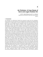
The third pattern appears when the wind flows with an angle of 90
o
. The vortex in that case
diminishes and the wind flows smoothly towards the domain exit, which indicates that the
removal efficiency of the domain local wind in that that pattern is the best over the above
two patterns. Results of the numerical approach for the pollutant concentration inside the
street canyon are displayed in Fig. 12. The figure shows the concentration fields at z = 0.05 m
for the five wind directions. In the case of normal wind, the concentration field shows
symmetry around the central section of the street. It is observed that, high concentration
regions appear inside the street canyon, while very low concentration regions appear
outside it. That note means that the domain local wind has no ability to carry the pollutants
outside the canyon.


0
o




30
o



45
o




60
o



90
o

x
y






































Fig. 12. Concentration fields for different wind directions (z = 0.05 m).

In the cases θ = 30
o
, 45

o
, and 60
o
, the concentration field increased to cover a wide area
outside the study domain due to pollutant diffusion towards the outside in the same wind
direction. As the maximum concentration area decreases with increasing θ, the canyon
averaged concentrations are expected to be lower than the concentration of the case of
normal wind as clean air continuously comes into the canyon from outside and dilutes the
domain polluted air. Also, it is observed that, very low concentrations exist in the lower part
of the figure where clean air arrives. In the case of θ = 90
o
, a large percentage of the
maximum concentration area is shifted outside the canyon, which indicates that the domain
average concentration in this case has the lowest value among all of the cases.
x
y
0
o
30
o
45
o
60
o
kg/kg

0.0018
0.0016
0.0015
0.0014

0.0013
0.0011
0.0010
0.0009
0.0008
0.0006
0.0005
0.0004
0.0002
0.0001
0.0000





90
o
Modeling of Ventilation Efciency 219

only one vortex appears at the right edge of the upwind building as the incoming wind
enters from that side. As the angle θ increases, the vortex size decreases and the flow
towards the domain exit in the y-direction increases. This pattern shows an improvement in
the domain wind removal efficiency compared with the case of normal wind.
































Fig. 11. Horizontal wind vector fields at different wind directions (z = 0.05 m).

The third pattern appears when the wind flows with an angle of 90
o
. The vortex in that case

diminishes and the wind flows smoothly towards the domain exit, which indicates that the
removal efficiency of the domain local wind in that that pattern is the best over the above
two patterns. Results of the numerical approach for the pollutant concentration inside the
street canyon are displayed in Fig. 12. The figure shows the concentration fields at z = 0.05 m
for the five wind directions. In the case of normal wind, the concentration field shows
symmetry around the central section of the street. It is observed that, high concentration
regions appear inside the street canyon, while very low concentration regions appear
outside it. That note means that the domain local wind has no ability to carry the pollutants
outside the canyon.


0
o




30
o


45
o




60
o




90
o

x
y






































Fig. 12. Concentration fields for different wind directions (z = 0.05 m).

In the cases θ = 30
o
, 45
o
, and 60
o
, the concentration field increased to cover a wide area
outside the study domain due to pollutant diffusion towards the outside in the same wind
direction. As the maximum concentration area decreases with increasing θ, the canyon
averaged concentrations are expected to be lower than the concentration of the case of
normal wind as clean air continuously comes into the canyon from outside and dilutes the
domain polluted air. Also, it is observed that, very low concentrations exist in the lower part
of the figure where clean air arrives. In the case of θ = 90
o

, a large percentage of the
maximum concentration area is shifted outside the canyon, which indicates that the domain
average concentration in this case has the lowest value among all of the cases.
x
y
0
o
30
o
45
o
60
o
kg/kg

0.0018
0.0016
0.0015
0.0014
0.0013
0.0011
0.0010
0.0009
0.0008
0.0006
0.0005
0.0004
0.0002
0.0001
0.0000






90
o
Air Quality220

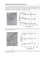
The three figures below presents the effects of the applied wind direction on the domain
average wind speed, domain pollutant concentrations and on the PFR, inside the study
domain. All quantities were normalized by the similar quantities evaluated at the case of
normal wind. Figure 13 displays the variation of the air quality parameters with the inflow
wind angle. The concentration decrease significantly to about 80% of its value as the flowing
wind angle changes from 0
o
to 90
o
. That behaviour can be attributed to the increased domain
average wind speed. That figure indicates that the domain average speed increases as the
wind angle increases it reaches to about 2.5 times as the flow becomes parallel. As the
average concentration inside the study domain decrease with increasing the applied wind
angle, while the domain volume is kept constant, the PFR is expected to increase. The figure
shows that the PFR increases by more than 6 times as the wind flow changes from 0
o
to 90
o
.
In addition, the trends of VF and TP demonstrate that the ventilation effectiveness within
the domain increases as the inflow wind angle increases.










(a)















(b)








0.00
0.05
0.10
0.15
0.20
0.25
0.30
0 10 20 30 40 50 60 70 80 90
C
p
x 100 (kg / m
3
)
Inlet wind angle (deg.)
0.0
0.4
0.8
1.2
1.6
2.0
0 10 20 30 40 50 60 70 80 90
PFR x 100 (m
3
/s)
Inlet wind angle (deg.)










(c)















(d)









Fig. 13. Air quality parameters within the study domain for variable wind directions; (a)
Domain averaged concentration, (b) Purging flow rate, (c) Visitation frequency, (d) Average
residence time

5.4. Effect of computational domain height (h)
This section is concerned with investigating the effect of the computational domain height (h)
on the VE indices of such domain. The height of the domain was started from 2 m and
increased gradually until 10 m, while the width D and the building height H were kept
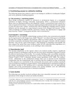
constant at 6 m and 10 m respectively. Figure 14 shows the concentration fields within the
street domain for four selected values of h/H (i.e. h/H = 0.2, 0.5, 0.8 and 1.0). Also, Fig. 15
shows the VE indices for different values of the domain height h. In these figures, it is clear
that the average concentration increases as the height of the computational domain increases,
which in turn decreases the air exchange rate within the domain. In the same time, the
0.0
0.4
0.8
1.2
1.6
2.0
0 10 20 30 40 50 60 70 80 90
VF
Inlet wind angle (deg.)
0.0
0.5
1.0
1.5
2.0
2.5

3.0
0 10 20 30 40 50 60 70 80 90
TP (s)
Inlet wind angle (deg.)
Modeling of Ventilation Efciency 221

The three figures below presents the effects of the applied wind direction on the domain
average wind speed, domain pollutant concentrations and on the PFR, inside the study
domain. All quantities were normalized by the similar quantities evaluated at the case of
normal wind. Figure 13 displays the variation of the air quality parameters with the inflow
wind angle. The concentration decrease significantly to about 80% of its value as the flowing
wind angle changes from 0
o
to 90
o
. That behaviour can be attributed to the increased domain
average wind speed. That figure indicates that the domain average speed increases as the
wind angle increases it reaches to about 2.5 times as the flow becomes parallel. As the
average concentration inside the study domain decrease with increasing the applied wind
angle, while the domain volume is kept constant, the PFR is expected to increase. The figure
shows that the PFR increases by more than 6 times as the wind flow changes from 0
o
to 90
o
.
In addition, the trends of VF and TP demonstrate that the ventilation effectiveness within
the domain increases as the inflow wind angle increases.










(a)















(b)








0.00
0.05
0.10
0.15
0.20
0.25
0.30
0 10 20 30 40 50 60 70 80 90
C
p
x 100 (kg / m
3
)
Inlet wind angle (deg.)
0.0
0.4
0.8
1.2
1.6
2.0
0 10 20 30 40 50 60 70 80 90
PFR x 100 (m
3
/s)
Inlet wind angle (deg.)










(c)















(d)








Fig. 13. Air quality parameters within the study domain for variable wind directions; (a)

Domain averaged concentration, (b) Purging flow rate, (c) Visitation frequency, (d) Average
residence time

5.4. Effect of computational domain height (h)
This section is concerned with investigating the effect of the computational domain height (h)
on the VE indices of such domain. The height of the domain was started from 2 m and
increased gradually until 10 m, while the width D and the building height H were kept
constant at 6 m and 10 m respectively. Figure 14 shows the concentration fields within the
street domain for four selected values of h/H (i.e. h/H = 0.2, 0.5, 0.8 and 1.0). Also, Fig. 15
shows the VE indices for different values of the domain height h. In these figures, it is clear
that the average concentration increases as the height of the computational domain increases,
which in turn decreases the air exchange rate within the domain. In the same time, the
0.0
0.4
0.8
1.2
1.6
2.0
0 10 20 30 40 50 60 70 80 90
VF
Inlet wind angle (deg.)
0.0
0.5
1.0
1.5
2.0
2.5
3.0
0 10 20 30 40 50 60 70 80 90
TP (s)

Inlet wind angle (deg.)
Air Quality222

variation of h has no considerable influence on the visitation frequency of the pollutants to the
domain. This can be attributed to the fact that both the domain inflow flux and domain’s
volume are increasing in nearly the same linear way, which is reflected in small changes in the
value of VF according to Equation (2). With the increase of domain’s volume, the residence
time is expected to become higher since the pollutants take more time to be flushed out of the
domain.








(a)








(b)










(c)








(d)

Fig. 14. Concentration fields within the street for different heights of the computational
domain (y/W = 0.5); (a) h/H = 0.2, (b) h/H = 0.5, (c) h/H = 0.8, (d) h/H = 1.0
x
z
kg/kg

0.1000
0.0928
0.0857
0.0785
0.0714
0.0642
0.0571

0.0500
0.0428
0.0357
0.0285
0.0214
0.0142
0.0071
0.0000









(a)
















(b)















(c)







0.00
0.05
0.10

0.15
0.20
0.2 0.3 0.4 0.5 0.6 0.7 0.8 0.9 1.0
C
p
(kg/m
3
)
h / H
0.0
0.5
1.0
1.5
2.0
2.5
3.0
0.2 0.3 0.4 0.5 0.6 0.7 0.8 0.9 1.0
Air exchange rate (1/h)×100
h /
H
0.0
0.5
1.0
1.5
2.0
2.5
3.0
0.2 0.3 0.4 0.5 0.6 0.7 0.8 0.9 1.0
VF
h /

H
Modeling of Ventilation Efciency 223

variation of h has no considerable influence on the visitation frequency of the pollutants to the
domain. This can be attributed to the fact that both the domain inflow flux and domain’s
volume are increasing in nearly the same linear way, which is reflected in small changes in the
value of VF according to Equation (2). With the increase of domain’s volume, the residence
time is expected to become higher since the pollutants take more time to be flushed out of the
domain.








(a)








(b)










(c)








(d)

Fig. 14. Concentration fields within the street for different heights of the computational
domain (y/W = 0.5); (a) h/H = 0.2, (b) h/H = 0.5, (c) h/H = 0.8, (d) h/H = 1.0
x
z
kg/kg

0.1000
0.0928
0.0857
0.0785
0.0714
0.0642
0.0571

0.0500
0.0428
0.0357
0.0285
0.0214
0.0142
0.0071
0.0000









(a)
















(b)















(c)







0.00
0.05
0.10

0.15
0.20
0.2 0.3 0.4 0.5 0.6 0.7 0.8 0.9 1.0
C
p
(kg/m
3
)
h / H
0.0
0.5
1.0
1.5
2.0
2.5
3.0
0.2 0.3 0.4 0.5 0.6 0.7 0.8 0.9 1.0
Air exchange rate (1/h)×100
h /
H
0.0
0.5
1.0
1.5
2.0
2.5
3.0
0.2 0.3 0.4 0.5 0.6 0.7 0.8 0.9 1.0
VF
h /

H
Air Quality224








(d)









Fig. 15. Effect of computational domain height on the VE indices (D = 6 m, H = 10 m); (a)
Domain averaged concentration, (b) Air exchange rate, (c) Visitation frequency, (d) Average
residence time.

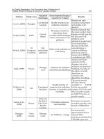
5.5 Effect of building array configurations
In this section, CFD simulations of the wind flow in densely urban areas – as an example of
applying the VE indices in evaluating the air quality of urban domain – are presented. In
this example, the VE indices are applied to one of the previously published works
(Davidson et al., 1996). Figure 16 shows two building array configurations – aligned and
staggered. The two configurations are fundamentally different as the staggered array diverts

flow onto neighbouring obstacles whereas the aligned array presents channels through
which the flow can pass (Davidson et al., 1996). The aligned array has 42 blocks, while the
staggered array is composed of 39 blocks. The dimensions of each block are: 2.3 m height
(H), 2.2 m width (W), and 2.45 m breadth (B).
To compare the wind ventilation performance for the two building patterns, seven domains
were considered within these arrays, domain (1 ~ 7), as shown in Fig. 16. Wind flow fields
were calculated for two directions of 0
o
and 45
o
. Figure 17 shows the flow fields around the
building patterns for the two directions.











0
20
40
60
80
100
0.2 0.3 0.4 0.5 0.6 0.7 0.8 0.9 1.0

TP (s)
h / H










θ = 0
o











θ = 45
o

(a)












θ = 0
o











θ = 45
o

(b)
Fig. 16. Schematic of two different building arrays showing the selected domains; (a) aligned,
(b) staggered.
2


5


7

2W

W/2

3


4


6


1













2
3

1

5

7
2B
4
6


Modeling of Ventilation Efciency 225








(d)










Fig. 15. Effect of computational domain height on the VE indices (D = 6 m, H = 10 m); (a)
Domain averaged concentration, (b) Air exchange rate, (c) Visitation frequency, (d) Average
residence time.

5.5 Effect of building array configurations
In this section, CFD simulations of the wind flow in densely urban areas – as an example of
applying the VE indices in evaluating the air quality of urban domain – are presented. In
this example, the VE indices are applied to one of the previously published works
(Davidson et al., 1996). Figure 16 shows two building array configurations – aligned and
staggered. The two configurations are fundamentally different as the staggered array diverts
flow onto neighbouring obstacles whereas the aligned array presents channels through
which the flow can pass (Davidson et al., 1996). The aligned array has 42 blocks, while the
staggered array is composed of 39 blocks. The dimensions of each block are: 2.3 m height
(H), 2.2 m width (W), and 2.45 m breadth (B).
To compare the wind ventilation performance for the two building patterns, seven domains
were considered within these arrays, domain (1 ~ 7), as shown in Fig. 16. Wind flow fields
were calculated for two directions of 0
o
and 45
o
. Figure 17 shows the flow fields around the
building patterns for the two directions.












0
20
40
60
80
100
0.2 0.3 0.4 0.5 0.6 0.7 0.8 0.9 1.0
TP (s)
h / H










θ = 0
o












θ = 45
o

(a)











θ = 0
o












θ = 45
o

(b)
Fig. 16. Schematic of two different building arrays showing the selected domains; (a) aligned,
(b) staggered.
2

5


7

2W

W/2

3


4



6


1












2
3

1

5

7
2B
4
6


Air Quality226


The calculated VE indices for the seven domains are shown in Fig. 18. The figure show large
variation in the air quality parameters. In the case of θ = 0
o
, the staggered array shows
undesirable air quality conditions within the selected domains compared with the case of
aligned blocks except for domains 3 and 4. High pollutant concentrations and low air
exchange rates are observed in this case. Additionally, the purging capability of the natural
wind for the staggered distribution was lower than that of the aligned one, reflected by high
values for VF and TP. This can be referred to the fact that the staggered distribution of
blocks prevents the direct flow between the blocks, which decreases the wind capability in
removing the pollutants. On the other hand, the smooth flow of the wind within the aligned
array at such wind direction dilutes the pollutant concentrations, and hence improves the air










(a)


















(b)



















(c)














(d)








Fig. 17. Wind flow fields around the two building arrays for the two directions (z/H = 0); (a)
aligned 0
o
, (a) staggered 0
o
, (a) aligned 45

o
, (a) staggered 0
o
.

quality of the considered domains. With respect to domains 3 and 4, the locations of such
domains within the aligned array are worse than their locations within the staggered one. The
geometry of the aligned blocks allows such domains to have three open boundaries, while in
the staggered distribution they have four boundaries. Such geometry decreases the ventilation
performance of the applied wind of these domains due to the lower inlet flux compared with
the other five domains. In the case of θ = 45
o
, the situation is reversed, where the staggered
array show good removal efficiency compared with the aligned array for almost all domains.
Such behavior can be attributed to the circulatory vortices that were established around the
aligned blocks at such wind direction. These circulatory flows decrease the wind ventilation
performance since it reduces the wind velocity within the array domains.
Modeling of Ventilation Efciency 227

The calculated VE indices for the seven domains are shown in Fig. 18. The figure show large
variation in the air quality parameters. In the case of θ = 0
o
, the staggered array shows
undesirable air quality conditions within the selected domains compared with the case of
aligned blocks except for domains 3 and 4. High pollutant concentrations and low air
exchange rates are observed in this case. Additionally, the purging capability of the natural
wind for the staggered distribution was lower than that of the aligned one, reflected by high
values for VF and TP. This can be referred to the fact that the staggered distribution of
blocks prevents the direct flow between the blocks, which decreases the wind capability in
removing the pollutants. On the other hand, the smooth flow of the wind within the aligned

array at such wind direction dilutes the pollutant concentrations, and hence improves the air










(a)

















(b)



















(c)















(d)








Fig. 17. Wind flow fields around the two building arrays for the two directions (z/H = 0); (a)
aligned 0
o
, (a) staggered 0
o
, (a) aligned 45
o
, (a) staggered 0
o
.

quality of the considered domains. With respect to domains 3 and 4, the locations of such
domains within the aligned array are worse than their locations within the staggered one. The
geometry of the aligned blocks allows such domains to have three open boundaries, while in
the staggered distribution they have four boundaries. Such geometry decreases the ventilation
performance of the applied wind of these domains due to the lower inlet flux compared with
the other five domains. In the case of θ = 45
o

, the situation is reversed, where the staggered
array show good removal efficiency compared with the aligned array for almost all domains.
Such behavior can be attributed to the circulatory vortices that were established around the
aligned blocks at such wind direction. These circulatory flows decrease the wind ventilation
performance since it reduces the wind velocity within the array domains.
Air Quality228

The results of such example show that the ventilation performance of the natural wind
within a domain may be changed for the same domain at different conditions of the incident
flow. In addition; the results shown confirm that the ventilation efficiency indices are able to
reflect the flow characteristics within urban domains very well.










(a)


















(b)













0.0
0.5
1.0
1.5
2.0
2.5
3.0

3.5
0 1 2 3 4 5 6 7 8
C
p
(kg/m
3
)×10
2
Domain (ID)
Aligned (0)
Staggered (0)
Aligned (45)
Staggered (45)
0.00
0.05
0.10
0.15
0.20
0.25
0.30
0 1 2 3 4 5 6 7 8
Air exchange rate (1/h)
Domain (ID)
Aligned (0)
Staggered (0)
Aligned (45)
Staggered (45)











(c)


















(d)









Fig. 18. Air quality parameters within selected domains for the two building arrays; (a)
Domain averaged concentration, (b) Air exchange rate, (c) Visitation frequency, (b) Average
staying time.

6. Conclusions
Ventilation efficiency indices of indoor environments were applied in evaluating the air
quality of urban domains. There are many indices which represent the ventilation efficiency
of indoor domains but three indices only are considered here: purging flow rate, visitation
frequency and residence time. The calculations of these indices were carried out based on
the average flow field analysis using computational fluid dynamics (CFD). Five case studies
1.0
1.2
1.4
1.6
1.8
2.0
0 1 2 3 4 5 6 7 8
VF
Domain (ID)
Aligned (0)
Staggered (0)
Aligned (45)
Staggered (45)
0
5

10
15
20
25
30
0 1 2 3 4 5 6 7 8
TP (s)
Domain (ID)
Aligned (0)
Staggered (0)
Aligned (45)
Staggered (45)



Modeling of Ventilation Efciency 229

The results of such example show that the ventilation performance of the natural wind
within a domain may be changed for the same domain at different conditions of the incident
flow. In addition; the results shown confirm that the ventilation efficiency indices are able to
reflect the flow characteristics within urban domains very well.











(a)

















(b)














0.0
0.5
1.0
1.5
2.0
2.5
3.0
3.5
0 1 2 3 4 5 6 7 8
C
p
(kg/m
3
)×10
2
Domain (ID)
Aligned (0)
Staggered (0)
Aligned (45)
Staggered (45)
0.00
0.05
0.10
0.15
0.20
0.25
0.30

0 1 2 3 4 5 6 7 8
Air exchange rate (1/h)
Domain (ID)
Aligned (0)
Staggered (0)
Aligned (45)
Staggered (45)










(c)



















(d)








Fig. 18. Air quality parameters within selected domains for the two building arrays; (a)
Domain averaged concentration, (b) Air exchange rate, (c) Visitation frequency, (b) Average
staying time.

6. Conclusions
Ventilation efficiency indices of indoor environments were applied in evaluating the air
quality of urban domains. There are many indices which represent the ventilation efficiency
of indoor domains but three indices only are considered here: purging flow rate, visitation
frequency and residence time. The calculations of these indices were carried out based on
the average flow field analysis using computational fluid dynamics (CFD). Five case studies
1.0
1.2
1.4
1.6
1.8

2.0
0 1 2 3 4 5 6 7 8
VF
Domain (ID)
Aligned (0)
Staggered (0)
Aligned (45)
Staggered (45)
0
5
10
15
20
25
30
0 1 2 3 4 5 6 7 8
TP (s)
Domain (ID)
Aligned (0)
Staggered (0)
Aligned (45)
Staggered (45)



Air Quality230

for evaluating the air quality of urban domain in terms of the VE indices were considered. In
the first and second cases, effects of the geometry of an isolated urban street (street width
and street building height) on the air quality within the street domain were investigated. In

the third one, the influence of wind direction on the air quality was investigated. In the
fourth case, the effect of the computational domain height was investigated. Finally, in the
fifth case, the effect of building arrangements on the air quality in dense urban areas was
studied.
In conclusions, it can be said that the ventilation efficiency indices of indoor environments
appear to be a promising tool in evaluating the air quality of urban domains as well. One of
the features of applying these indices is that it is not necessary to consider the location of the
pollutant source within the study domain. In addition, the VE indices are able to describe
the pollutant behavior within the domain, which is very important for obtaining a complete
assessment for the wind ventilation performance within urban domains.

7. References
Chock, D. (1977). A simple line-source model for dispersion near roadways, Atmospheric
Environment, Vol. 12(4), pp. 823-829.
Sandberg, M. (1992). Ventilation effectiveness and purging flow rate – A review,
Proceedings
of the International Symposium on Room Air Convection and Ventilation Effectiveness;
pp. 1-21, Tokyo, Japan.
Ito, K.; Kato S., & Murakami, S. (2000). Study of visitation frequency and purging flow rate
based on averaged contaminant distribution–Study on evaluating of ventilation
effectiveness of occupied space in room,
Japanese Journal of Architecture Planning and
Environmental Engineering (Transaction of AIJ)
, Vol. 529, pp. 31-37, (in Japanese).
Kato, S.; Ito, K. & Murakami, S. (2003). Analysis of visitation frequency through particle
tracking method based on LES and model experiment,
Indoor Air, Vol. 13 (2), pp.
182-193.
Uehara, K.; Murakami, S.; Oikawa, S. & Wakamatsu, S. (1997). Wind tunnel test of
concentration fields around street canyons within the stratified urban canopy layer,

Part 3: Experimental studies on gaseous diffusion in urban areas;
Journal of
Architecture Planning and Environmental Engineering (Transaction of AIJ)
, Vol. 499, pp.
9-16 (in Japanese).
Huang, H.; Ooka, R.; Kato, S. & Jiang, T. (2006). CFD analysis of ventilation efficiency
around an elevated highway using visitation frequency and purging flow rate,
Journal of Wind and Structure, Vol. 9 (4).
Sandberg, M. (1983). The use of moments for ventilation assessing air quality in ventilated
Room,
Building and Environment, Vol. 18 (4), pp. 181-197.
Kato, S. & Murakami, S. (1992). New scales for ventilation efficiency and their application
based on numerical simulation and of room airflow,
Proceedings of ISRACVE, The
University of Tokyo, Japan, pp. 22-37.
Mfula, A.; Kukadia, V.; Griffiths, R. & Hall D (2005). Wind tunnel modelling of urban
building exposure to outdoor pollution,
Atmospheric Environment; Vol. 39 (15), pp.
2737-2745.

He, P.; Katayama, T.; Hayashi, T., Tanimoto, J. & Hosooka, I. (1997). Numerical simulation
of air flow in an urban area with regularly aligned blocks,
Journal of Wind
Engineering and Industrial Aerodynamics
, Vol. 67&68, pp. 281-291.
Lien, S.; Yee, E. & Cheng, Y. (2004). Simulation of mean flow and turbulence over a 2-D
building array using high resolution CFD and a distributed drag force approach,
Journal of Wind Engineering and Industrial Aerodynamics, Vol. 92, pp. 117-158.
Kim, J. & Baik, J. (2004). A numerical study of the effects of ambient wind direction on flow
and dispersion in urban street canyon using the RNG k-ε turbulent model,

Atmospheric Environment, Vol. 38, pp. 3039-3048.
Ferzigere, J. & Peric, M. (1997). Computational methods for fluid dynamics, Springer, Third
Edition.
Xiaomin, X.; Zhen, H. & Jia, S. (2005). Impact of building configuration on air quality in
street canyon,
Atmospheric Environment, Vol. 39 (25), pp. 4519-4530.
Kanda, I.; Uehara, K.; Yamao, Y.; Yoshikawa, Y., & Morikawa, T. (2006). A wind tunnel
study on exhaust gas dispersion from road vehicles -Part II: Effect of vehicle
queues,
Journal of Wind Engineering and Industrial Aerodynamics, Vol. 94(9), pp. 659-
673.
Tsai, Y. & Chen, S. (2004). Measurements and three-dimensional modelling of air pollutant
dispersion in an urban street canyon,
Atmospheric Environment; Vol. 38(35), pp.
5911-5924.
Baker, C. J. & Hargreaves, D. M. (2001). Wind tunnel evaluation of a vehicle pollution
dispersion model,
Journal of Wind Engineering and Industrial Aerodynamics; Vol. 89(2),
pp. 187-200.
Ahmad, K.; Khare, M. & Chaudhry, K. (2005). Wind tunnel simulation studies on dispersion
at urban street canyons and intersections- A review,
Journal of Wind Engineering and
Industrial Aerodynamics
; Vol. 93 (9), pp. 697-717.
Bady, M.; Kato, S.; Takahashi, T. & Huang, H. (2008). An experimental investigation of the
wind environment and air quality within a densely populated urban street canyon.
Submitted.
Bady, M.; Kato, S.; Ishida, Y.; Huang, H; & Takahashi, T. (2008). Exceedance probability as a
tool to evaluate the wind environment within densely urban areas”.
Journal of Wind

and Structure, Vol. 11(6).
Hui, S.; & Davidson, L. (1997). Towards the determination of the local purging flow rate,
Building and Environment; Vol. 32(6), pp. 513-525.
Bady, M.; Kato, S.; & Huang, H. (2008). Towards the application of indoor ventilation
efficiency indices to evaluate the air quality of urban areas,
Building and
Environment, Vol. 43(12).
Davidson, M.; Snyder, W.; Lawson R. & Hunt J. (1996). Wind tunnel simulation of plume
dispersion through groups of obstacles,
Atmospheric Environment; Vol. 30(22), pp.
3715-3731.


Modeling of Ventilation Efciency 231

for evaluating the air quality of urban domain in terms of the VE indices were considered. In
the first and second cases, effects of the geometry of an isolated urban street (street width
and street building height) on the air quality within the street domain were investigated. In
the third one, the influence of wind direction on the air quality was investigated. In the
fourth case, the effect of the computational domain height was investigated. Finally, in the
fifth case, the effect of building arrangements on the air quality in dense urban areas was
studied.
In conclusions, it can be said that the ventilation efficiency indices of indoor environments
appear to be a promising tool in evaluating the air quality of urban domains as well. One of
the features of applying these indices is that it is not necessary to consider the location of the
pollutant source within the study domain. In addition, the VE indices are able to describe
the pollutant behavior within the domain, which is very important for obtaining a complete
assessment for the wind ventilation performance within urban domains.

7. References

Chock, D. (1977). A simple line-source model for dispersion near roadways, Atmospheric
Environment, Vol. 12(4), pp. 823-829.
Sandberg, M. (1992). Ventilation effectiveness and purging flow rate – A review,
Proceedings
of the International Symposium on Room Air Convection and Ventilation Effectiveness;
pp. 1-21, Tokyo, Japan.
Ito, K.; Kato S., & Murakami, S. (2000). Study of visitation frequency and purging flow rate
based on averaged contaminant distribution–Study on evaluating of ventilation
effectiveness of occupied space in room,
Japanese Journal of Architecture Planning and
Environmental Engineering (Transaction of AIJ)
, Vol. 529, pp. 31-37, (in Japanese).
Kato, S.; Ito, K. & Murakami, S. (2003). Analysis of visitation frequency through particle
tracking method based on LES and model experiment,
Indoor Air, Vol. 13 (2), pp.
182-193.
Uehara, K.; Murakami, S.; Oikawa, S. & Wakamatsu, S. (1997). Wind tunnel test of
concentration fields around street canyons within the stratified urban canopy layer,
Part 3: Experimental studies on gaseous diffusion in urban areas;
Journal of
Architecture Planning and Environmental Engineering (Transaction of AIJ)
, Vol. 499, pp.
9-16 (in Japanese).
Huang, H.; Ooka, R.; Kato, S. & Jiang, T. (2006). CFD analysis of ventilation efficiency
around an elevated highway using visitation frequency and purging flow rate,
Journal of Wind and Structure, Vol. 9 (4).
Sandberg, M. (1983). The use of moments for ventilation assessing air quality in ventilated
Room,
Building and Environment, Vol. 18 (4), pp. 181-197.
Kato, S. & Murakami, S. (1992). New scales for ventilation efficiency and their application

based on numerical simulation and of room airflow,
Proceedings of ISRACVE, The
University of Tokyo, Japan, pp. 22-37.
Mfula, A.; Kukadia, V.; Griffiths, R. & Hall D (2005). Wind tunnel modelling of urban
building exposure to outdoor pollution,
Atmospheric Environment; Vol. 39 (15), pp.
2737-2745.

He, P.; Katayama, T.; Hayashi, T., Tanimoto, J. & Hosooka, I. (1997). Numerical simulation
of air flow in an urban area with regularly aligned blocks,
Journal of Wind
Engineering and Industrial Aerodynamics
, Vol. 67&68, pp. 281-291.
Lien, S.; Yee, E. & Cheng, Y. (2004). Simulation of mean flow and turbulence over a 2-D
building array using high resolution CFD and a distributed drag force approach,
Journal of Wind Engineering and Industrial Aerodynamics, Vol. 92, pp. 117-158.
Kim, J. & Baik, J. (2004). A numerical study of the effects of ambient wind direction on flow
and dispersion in urban street canyon using the RNG k-ε turbulent model,
Atmospheric Environment, Vol. 38, pp. 3039-3048.
Ferzigere, J. & Peric, M. (1997). Computational methods for fluid dynamics, Springer, Third
Edition.
Xiaomin, X.; Zhen, H. & Jia, S. (2005). Impact of building configuration on air quality in
street canyon,
Atmospheric Environment, Vol. 39 (25), pp. 4519-4530.
Kanda, I.; Uehara, K.; Yamao, Y.; Yoshikawa, Y., & Morikawa, T. (2006). A wind tunnel
study on exhaust gas dispersion from road vehicles -Part II: Effect of vehicle
queues,
Journal of Wind Engineering and Industrial Aerodynamics, Vol. 94(9), pp. 659-
673.
Tsai, Y. & Chen, S. (2004). Measurements and three-dimensional modelling of air pollutant

dispersion in an urban street canyon,
Atmospheric Environment; Vol. 38(35), pp.
5911-5924.
Baker, C. J. & Hargreaves, D. M. (2001). Wind tunnel evaluation of a vehicle pollution
dispersion model,
Journal of Wind Engineering and Industrial Aerodynamics; Vol. 89(2),
pp. 187-200.
Ahmad, K.; Khare, M. & Chaudhry, K. (2005). Wind tunnel simulation studies on dispersion
at urban street canyons and intersections- A review,
Journal of Wind Engineering and
Industrial Aerodynamics
; Vol. 93 (9), pp. 697-717.
Bady, M.; Kato, S.; Takahashi, T. & Huang, H. (2008). An experimental investigation of the
wind environment and air quality within a densely populated urban street canyon.
Submitted.
Bady, M.; Kato, S.; Ishida, Y.; Huang, H; & Takahashi, T. (2008). Exceedance probability as a
tool to evaluate the wind environment within densely urban areas”.
Journal of Wind
and Structure, Vol. 11(6).
Hui, S.; & Davidson, L. (1997). Towards the determination of the local purging flow rate,
Building and Environment; Vol. 32(6), pp. 513-525.
Bady, M.; Kato, S.; & Huang, H. (2008). Towards the application of indoor ventilation
efficiency indices to evaluate the air quality of urban areas,
Building and
Environment, Vol. 43(12).
Davidson, M.; Snyder, W.; Lawson R. & Hunt J. (1996). Wind tunnel simulation of plume
dispersion through groups of obstacles,
Atmospheric Environment; Vol. 30(22), pp.
3715-3731.



Air Quality232
Nonlocal-closure schemes for use in air quality and environmental models 233
Nonlocal-closure schemes for use in air quality and environmental
models
Dragutin T. Mihailović and Ana Firanja

X

Nonlocal-closure schemes for use in
air quality and environmental models

Dragutin T. Mihailović and Ana Firanj
Faculty of Agriculture, University of Novi Sad, Novi Sad, SERBIA
Dositeja Obradovića Sq. 8, 21000 Novi Sad

1. Introduction
The description of the atmospheric boundary layer (ABL) processes, understanding of
complex boundary layer interactions, and their proper parameterization are important for
air quality as well as many other environmental models. In that sense single-column
vertical mixing models are comprehensive enough to describe processes in ABL. Therefore,
they can be employed to illustrate the basic concepts on boundary layer processes and
represent serviceable tools in boundary layer investigation. When coupled to 3D models,
single-column models can provide detailed and accurate simulations of the ABL structure
as well as mixing processes.
Description of the ABL during convective conditions has long been a major source of
uncertainty in the air quality models and chemical transport models. There exist two
approaches, local and nonlocal, for solving the turbulence closure problem. While the local
closure assumes that turbulence is analogous to molecular diffusion in the nonlocal-closure,
the unknown quantity at one point is parameterized by values of known quantities at many

points in space. The simplest, most popular local closure method in Eulerian air quality and
chemical transport models is the K-Scheme used both in the boundary layer and the free
troposphere. Since it uses local gradients in one point of model grid, K-Scheme can be used
only when the scale of turbulent motion is much smaller than the scale of mean flow (Stull,
1988), such as in the case of stable and neutral conditions in the atmosphere in which this
scheme is consistent. However, it can not: (a) describe the effects of large scale eddies that
are dominant in the convective boundary layer (CBL) and (b) simulate counter-gradient
flows where a turbulent flux flows up to the gradient. Thus, K-Scheme is not recommended
in the CBL (Stull, 1988). Recently, in order to avoid the K-scheme drawbacks, Alapaty
(Alapaty, 2003; Alapaty & Alapaty, 2001) suggested a “nonlocal” turbulent kinetic energy
(TKE) scheme based on the K-Scheme that was intensively tested using the EMEP chemical
transport model (Mihailovic & Jonson, 2005; Mihailovic & Alapaty, 2007). In order to
quantify the transport of a passive tracer field in three-dimensional simulations of turbulent
convection, the nonlocal and non-diffusive behavior can be described by a transilient matrix
whose elements contain the fractional tracer concentrations moving from one subvolume to
another as a function of time. The approach was originally developed for and applied to
geophysical flows known as turbulent transilient theory (T3) (Stull, 1988; Stull & Driedonks,
10
Air Quality234

1987; Alapaty et al., 1997), but this formalism was extended and applied in an astrophysical
context to three-dimensional simulations of turbulent compressible convection with
overshoot into convectively stable bounding regions (Miesch et al., 2000). The most
frequently used nonlocal-closure method is the asymmetric convective model (ACM)
suggested by Pleim & Chang (1992). The design of this model is based on the Blackadar’s
scheme (Blackadar, 1976), but takes into account the important fact that, in the CBL, the
vertical transport is asymmetrical (Wyngaard & Brost, 1984). Namely, the buoyant plumbs
are rather fast and narrow, while downward streams are wide and slow. Accordingly,
transport by upward streams should be simulated as nonlocal and transport by downward
streams as local. The concept of this model is that buoyant plumbs rise from the surface

layer and transfer air and its properties directly into all layers above. Downward mixing
occurs only between adjacent layers in the form of a slow subsidence. The ACM can be used
only during convective conditions in the ABL, while stable or neutral regimes for the K-
Scheme are considered. Although this approach results in a more realistic simulation of
vertical transport within the CBL, it has some drawbacks that can be elaborated in
condensed form: (i) since this method mixes the same amount of mass to every vertical layer
in the boundary layer, it has the potential to remove mass much too quickly out of the
surface layer and (ii) this method fails to account for the upward mixing in layers higher
than the surface layer (Tonnesen et al., 1998). Wang (Wang, 1998) has compared three
different vertical transport methods: a semi-implicit K-Scheme (SIK) with local closure and
the ACM and T3 schemes with nonlocal-closure. Of the three schemes, the ACM scheme
moved mass more rapidly out of surface layer into other layers than the other two schemes
in terms of the rate at which mass was mixed between different layers. Recently, this scheme
was modified with varying upward mixing rates (VUR), where the upward mixing rate
changes with the height, providing slower mixing (Mihailović et al., 2008).
The aim of this chapter is to give a short overview of nonlocal-closure TKE and ABL mixing
schemes developed to describe vertical mixing during convective conditions in the ABL. The
overview is supported with simulations performed by the chemical EMEP Unied model
(version UNI-ACID, rv2.0) where schemes were incorporated.

2. Description of nonlocal-closure schemes
2.1. Turbulent kinetic energy scheme (TKE)
As we mentioned above the well-known issues regarding local-closure ABL schemes is their
inability to produce well-mixed layers in the ABL during convective conditions. Holtslag &
Boville (1993) using the NCAR Community Climate Model (CCM2) studied a classic
example of artifacts resulting from the deficiencies in the first-order closure schemes. To
alleviate problems associated with the general first-order eddy-diffusivity
K -schemes, they
proposed a nonlocal K -scheme. Hong & Pan (1996) presented an enhanced version of the
Holtslag & Boville (1993) scheme. In this scheme the friction velocity scale ( u


) is used as a
closure in their formulation. However, for moderate to strong convective conditions,
u


is
not a representative scale (Alapaty & Alapaty, 2001). Rather, the convective velocity ( w

)
scale is suitable as used by Hass et al. (1991) in simulation of a wet deposition case in Europe
by the European Acid Deposition Model (EURAD). Depending on the magnitude of the
scaling parameter h L ( h is height of the ABL, and L is Monin-Obukhov length), either

u

or w

is used in many other formulations. Notice that this approach may not guarantee
continuity between the alternate usage of
u

and w

in estimating K - eddy diffusivity.
Also, in most of the local-closure schemes the coefficient of vertical eddy diffusivity for
moisture is assumed to be equal to that for heat. Sometimes this assumption leads to vertical
gradients in the simulated moisture fields, even during moderate to strong convective
conditions in the ABL. Also, the nonlocal scheme considers the horizontal advection of
turbulence that may be important over heterogeneous landscapes (Alapaty & Alapaty, 2001;

Mihailovic et al. 2005).
The starting point of approach is to consider the general form of the vertical eddy diffusivity
equation. For momentum, this equation can be written as



 

 
 

1
Ф
p
m
m
z
e kz
h
K

(1)

where
m
K is the vertical eddy diffusivity, e

is the mean turbulent velocity scale within the
ABL to be determined (closure problem), k is the von Karman constant ( k


0.41 ), z is the
vertical coordinate,
p
is the profile shape exponent coming from the similarity theory (Troen
& Mahrt, 1986; usually taken as 2), and
m
Ф is the nondimensional function of momentum.
According to Zhang et al. (1996), we use the square root of the vertically averaged turbulent
kinetic energy in the ABL as a velocity scale, in place of the mean wind speed, the closure to
Eq. (1). Instead of using a prognostic approach to determine TKE, we make use of a
diagnostic method. It is then logical to consider the diagnostic TKE to be a function of both
u

and w

. Thus, the square root of diagnosed TKE near the surface serves as a closure to
this problem (Alapaty & Alapaty, 2001). However, it is more suitable to estimate
e

from the
profile of the TKE through the whole ABL.
According to Moeng & Sullivan (1994), a linear combination of the turbulent kinetic energy
dissipation rates associated with shear and buoyancy can adequately approximate the
vertical distribution of the turbulent kinetic energy,


e z , in a variety of boundary layers
ranging from near neutral to free convection conditions. Following Zhang et al. (1996) the
TKE profile can be expressed as



   
 
 
 
  
 
 
   
2 3
2 3
3 3
Ф1
0.4 ,
2
m
E
L
e z w u h z
h kz
(2)

where
E
L characterizes the integral length scale of the dissipation rate. Here,
 
m
z L

 

1 4
Ф 1 15 / is an empirical function for the unstable atmospheric surface layer
(Businger et al., 1971), which is applied to both the surface and mixed layer. We used
E
L h 2.6 which is in the range h h

2.5 3.0 suggested by Moeng & Sullivan (1994). For the
stable atmospheric boundary layer we modeled the TKE profile using an empirical function
proposed by Lenschow et al. (1988), based on aircraft observations
Nonlocal-closure schemes for use in air quality and environmental models 235

1987; Alapaty et al., 1997), but this formalism was extended and applied in an astrophysical
context to three-dimensional simulations of turbulent compressible convection with
overshoot into convectively stable bounding regions (Miesch et al., 2000). The most
frequently used nonlocal-closure method is the asymmetric convective model (ACM)
suggested by Pleim & Chang (1992). The design of this model is based on the Blackadar’s
scheme (Blackadar, 1976), but takes into account the important fact that, in the CBL, the
vertical transport is asymmetrical (Wyngaard & Brost, 1984). Namely, the buoyant plumbs
are rather fast and narrow, while downward streams are wide and slow. Accordingly,
transport by upward streams should be simulated as nonlocal and transport by downward
streams as local. The concept of this model is that buoyant plumbs rise from the surface
layer and transfer air and its properties directly into all layers above. Downward mixing
occurs only between adjacent layers in the form of a slow subsidence. The ACM can be used
only during convective conditions in the ABL, while stable or neutral regimes for the K-
Scheme are considered. Although this approach results in a more realistic simulation of
vertical transport within the CBL, it has some drawbacks that can be elaborated in
condensed form: (i) since this method mixes the same amount of mass to every vertical layer
in the boundary layer, it has the potential to remove mass much too quickly out of the
surface layer and (ii) this method fails to account for the upward mixing in layers higher
than the surface layer (Tonnesen et al., 1998). Wang (Wang, 1998) has compared three

different vertical transport methods: a semi-implicit K-Scheme (SIK) with local closure and
the ACM and T3 schemes with nonlocal-closure. Of the three schemes, the ACM scheme
moved mass more rapidly out of surface layer into other layers than the other two schemes
in terms of the rate at which mass was mixed between different layers. Recently, this scheme
was modified with varying upward mixing rates (VUR), where the upward mixing rate
changes with the height, providing slower mixing (Mihailović et al., 2008).
The aim of this chapter is to give a short overview of nonlocal-closure TKE and ABL mixing
schemes developed to describe vertical mixing during convective conditions in the ABL. The
overview is supported with simulations performed by the chemical EMEP Unied model
(version UNI-ACID, rv2.0) where schemes were incorporated.

2. Description of nonlocal-closure schemes
2.1. Turbulent kinetic energy scheme (TKE)
As we mentioned above the well-known issues regarding local-closure ABL schemes is their
inability to produce well-mixed layers in the ABL during convective conditions. Holtslag &
Boville (1993) using the NCAR Community Climate Model (CCM2) studied a classic
example of artifacts resulting from the deficiencies in the first-order closure schemes. To
alleviate problems associated with the general first-order eddy-diffusivity
K -schemes, they
proposed a nonlocal K -scheme. Hong & Pan (1996) presented an enhanced version of the
Holtslag & Boville (1993) scheme. In this scheme the friction velocity scale ( u

) is used as a
closure in their formulation. However, for moderate to strong convective conditions,
u


is
not a representative scale (Alapaty & Alapaty, 2001). Rather, the convective velocity ( w


)
scale is suitable as used by Hass et al. (1991) in simulation of a wet deposition case in Europe
by the European Acid Deposition Model (EURAD). Depending on the magnitude of the
scaling parameter h L ( h is height of the ABL, and L is Monin-Obukhov length), either

u

or w

is used in many other formulations. Notice that this approach may not guarantee
continuity between the alternate usage of
u

and w

in estimating K - eddy diffusivity.
Also, in most of the local-closure schemes the coefficient of vertical eddy diffusivity for
moisture is assumed to be equal to that for heat. Sometimes this assumption leads to vertical
gradients in the simulated moisture fields, even during moderate to strong convective
conditions in the ABL. Also, the nonlocal scheme considers the horizontal advection of
turbulence that may be important over heterogeneous landscapes (Alapaty & Alapaty, 2001;
Mihailovic et al. 2005).
The starting point of approach is to consider the general form of the vertical eddy diffusivity
equation. For momentum, this equation can be written as



 

 

 

1
Ф
p
m
m
z
e kz
h
K

(1)

where
m
K is the vertical eddy diffusivity, e

is the mean turbulent velocity scale within the
ABL to be determined (closure problem),
k is the von Karman constant ( k  0.41 ), z is the
vertical coordinate,
p
is the profile shape exponent coming from the similarity theory (Troen
& Mahrt, 1986; usually taken as 2), and
m
Ф is the nondimensional function of momentum.
According to Zhang et al. (1996), we use the square root of the vertically averaged turbulent
kinetic energy in the ABL as a velocity scale, in place of the mean wind speed, the closure to
Eq. (1). Instead of using a prognostic approach to determine TKE, we make use of a

diagnostic method. It is then logical to consider the diagnostic TKE to be a function of both
u

and w

. Thus, the square root of diagnosed TKE near the surface serves as a closure to
this problem (Alapaty & Alapaty, 2001). However, it is more suitable to estimate
e

from the
profile of the TKE through the whole ABL.
According to Moeng & Sullivan (1994), a linear combination of the turbulent kinetic energy
dissipation rates associated with shear and buoyancy can adequately approximate the
vertical distribution of the turbulent kinetic energy,


e z , in a variety of boundary layers
ranging from near neutral to free convection conditions. Following Zhang et al. (1996) the
TKE profile can be expressed as


   
 
 
 
  
 
 
   
2 3

2 3
3 3
Ф1
0.4 ,
2
m
E
L
e z w u h z
h kz
(2)

where
E
L characterizes the integral length scale of the dissipation rate. Here,
 
m
z L

 
1 4
Ф 1 15 / is an empirical function for the unstable atmospheric surface layer
(Businger et al., 1971), which is applied to both the surface and mixed layer. We used
E
L h 2.6 which is in the range h h2.5 3.0 suggested by Moeng & Sullivan (1994). For the
stable atmospheric boundary layer we modeled the TKE profile using an empirical function
proposed by Lenschow et al. (1988), based on aircraft observations
Air Quality236



 

 
 
 
 
1.75
2
6 1 .
e z
z
h
u
(3)

Following LES (Large Eddy Simulation) works of Zhang et al. (1996) and Moeng & Sullivan
(1994), Alapaty (2003) suggested how to estimate the vertically integrated mean turbulent
velocity scale
e

that within the ABL can be written as


   

 

0
1
,

h
e e z z dz
h
(4)

where
 
z is the vertical profile function for turbulent kinetic energy as obtained by Zhang
et al. (1996) based on LES studies, later modified by Alapaty (personal communication), and
dz is layer thickness.
The formulation of eddy-diffusivity by Eq. (1) depends on
h . We follow Troen & Mahrt
(1986) for determination of
h using


   


 
 
 




2 2
0
,
c

v s
Ri u h v h
h
g
h
(5)

where
c
Ri is a critical bulk Richardson number for the ABL,


u h and


v h are the
horizontal velocity components at
h g

0
, / , is the buoyancy parameter,

0
is the appropriate
virtual potential temperature, and


v
h


is the virtual potential temperature of air near the
surface at
h , respectively. For unstable conditions


s
L

 0 , is given by (Troen & Mahrt
(1986))

 

 
 
0
1 0
v
s v
s
w
z C
w
, (6)

where
C 
0
8.5 (Holtslag et al., 1990),
s

w is the velocity while
v
w

0
is the kinematics surface
heat flux. The velocity
s
w is parameterized as




 
 
1 3
3 3
1s
w u c w

(7)
and

 
 

 

 
1 3

0 0
/
v
w g w h
.

(8)

Using c 
1
0.6 . In Eq. (6),


v
z

1
is the virtual temperature at the first model level. The
second term on the right-hand side of Eq. (6) represents a temperature excess, which is a
measure in the lower part of the ABL. For stable conditions we use


s v
z
 

1
with z 
1
2 m.


On the basis of Eq. (5) the height of the ABL can be calculated by iteration for all stability
conditions, when the surface fluxes and profiles of
v

, u and v are known. The
computation starts with calculating the bulk Richardson number
Ri between the level
s

and subsequent higher levels of the model. Once Ri exceeds the critical value, the value
of
h is derived with linear interpolation between the level with
c
Ri Ri and the level
underneath. We use a minimum of 100 m for
h . In Eq. (5),
c
Ri is the value of the critical bulk
Richardson number used to be 0.25 in this study.
In the free atmosphere, turbulent mixing is parameterized using the formulation suggested
by Blackadar (1979) in which vertical eddy diffusivities are functions of the Richardson
number and wind shear in the vertical. This formulation can be written as


 

 
2
0m

Rc Ri
K K S kl
Rc
,

(9)

where
K
0
is the background value (1 m
2
s
-1
), S is the vertical wind shear, l is the
characteristic turbulent length scale (100 m),
Rc is the critical Richardson number, and Ri
is the Richardson number defined as







2
v
v
g
Ri

z
S
. (10)

The critical Richardson number in Eq. (9) is determined as


 
 
0.175
0.257Rc z ,

(11)

where
z is the layer thickness (Zhang & Anthes, 1982).

2.2. Nonlocal vertical mixing schemes
The nonlocal vertical mixing schemes were designed to describe the effects of large scale
eddies, that are dominant in the CBL and to simulate counter-gradient flows where a
turbulent flux flows up to the gradient. During convective conditions in the atmosphere,
both small-scale subgrid and large-scale super grid eddies are important for vertical
transport. In this section, we will consider three different nonlocal mixing schemes: the
Blackadar’s scheme (Blackadar, 1976), the asymmetrical convective model (Pleim & Chang,
1992) and the scheme with varying upward mixing rates (Mihailovic et al., 2008).
Transilient turbulence theory (Stull, 1988) (the Latin word
transilient means to jump over) is
a general representation of the turbulent flux exchange processes. In transilient mixing
schemes, elements of flux exchange are defined in an
N N


transilient matrix, where N is
the number of vertical layers and mixing occurs not only between adjacent model layers, but
also between layers not adjacent to each other. That means that all of the matrix elements are
nonzero and that the turbulent mixing in the convective boundary layer can be written as

Nonlocal-closure schemes for use in air quality and environmental models 237





 
 
 
 
1.75
2
6 1 .
e z
z
h
u
(3)

Following LES (Large Eddy Simulation) works of Zhang et al. (1996) and Moeng & Sullivan
(1994), Alapaty (2003) suggested how to estimate the vertically integrated mean turbulent
velocity scale
e


that within the ABL can be written as


   

 

0
1
,
h
e e z z dz
h
(4)

where
 
z is the vertical profile function for turbulent kinetic energy as obtained by Zhang
et al. (1996) based on LES studies, later modified by Alapaty (personal communication), and
dz is layer thickness.
The formulation of eddy-diffusivity by Eq. (1) depends on
h . We follow Troen & Mahrt
(1986) for determination of
h using


   


 

 
 




2 2
0
,
c
v s
Ri u h v h
h
g
h
(5)

where
c
Ri is a critical bulk Richardson number for the ABL,


u h and


v h are the
horizontal velocity components at
h g

0

, / , is the buoyancy parameter,

0
is the appropriate
virtual potential temperature, and


v
h

is the virtual potential temperature of air near the
surface at h , respectively. For unstable conditions


s
L

 0 , is given by (Troen & Mahrt
(1986))

 

 
 
0
1 0
v
s v
s
w

z C
w
, (6)

where
C 
0
8.5 (Holtslag et al., 1990),
s
w is the velocity while
v
w

0
is the kinematics surface
heat flux. The velocity
s
w is parameterized as




 
 
1 3
3 3
1s
w u c w

(7)

and

 
 






1 3
0 0
/
v
w g w h
.

(8)

Using c 
1
0.6 . In Eq. (6),


v
z

1
is the virtual temperature at the first model level. The
second term on the right-hand side of Eq. (6) represents a temperature excess, which is a

measure in the lower part of the ABL. For stable conditions we use


s v
z
 

1
with z 
1
2 m.

On the basis of Eq. (5) the height of the ABL can be calculated by iteration for all stability
conditions, when the surface fluxes and profiles of
v

, u and v are known. The
computation starts with calculating the bulk Richardson number
Ri between the level
s

and subsequent higher levels of the model. Once Ri exceeds the critical value, the value
of
h is derived with linear interpolation between the level with
c
Ri Ri and the level
underneath. We use a minimum of 100 m for
h . In Eq. (5),
c
Ri is the value of the critical bulk

Richardson number used to be 0.25 in this study.
In the free atmosphere, turbulent mixing is parameterized using the formulation suggested
by Blackadar (1979) in which vertical eddy diffusivities are functions of the Richardson
number and wind shear in the vertical. This formulation can be written as


 

 
2
0m
Rc Ri
K K S kl
Rc
,

(9)

where
K
0
is the background value (1 m
2
s
-1
), S is the vertical wind shear, l is the
characteristic turbulent length scale (100 m),
Rc is the critical Richardson number, and Ri
is the Richardson number defined as








2
v
v
g
Ri
z
S
. (10)

The critical Richardson number in Eq. (9) is determined as


 
 
0.175
0.257Rc z ,

(11)

where
z is the layer thickness (Zhang & Anthes, 1982).

2.2. Nonlocal vertical mixing schemes
The nonlocal vertical mixing schemes were designed to describe the effects of large scale

eddies, that are dominant in the CBL and to simulate counter-gradient flows where a
turbulent flux flows up to the gradient. During convective conditions in the atmosphere,
both small-scale subgrid and large-scale super grid eddies are important for vertical
transport. In this section, we will consider three different nonlocal mixing schemes: the
Blackadar’s scheme (Blackadar, 1976), the asymmetrical convective model (Pleim & Chang,
1992) and the scheme with varying upward mixing rates (Mihailovic et al., 2008).
Transilient turbulence theory (Stull, 1988) (the Latin word
transilient means to jump over) is
a general representation of the turbulent flux exchange processes. In transilient mixing
schemes, elements of flux exchange are defined in an
N N transilient matrix, where N is
the number of vertical layers and mixing occurs not only between adjacent model layers, but
also between layers not adjacent to each other. That means that all of the matrix elements are
nonzero and that the turbulent mixing in the convective boundary layer can be written as

Air Quality238







1
N
i
i
j j
j
c

M
c
t
, (12)

where
c is the concentration of passive tracer, the elements in the mixing matrix M represent
mass mixing rates, and
i and j refer to two different grid cells in a column of atmosphere.
Some models specify mixing concepts with the idea of reducing the number of nonzero
elements because of the cost of computational time during integration.
The Blackadar’s scheme (Blackadar, 1976) is a simple nonlocal-closure scheme, that is designed
to describe convective vertical transport by eddies of varying sizes. The effect of convective
plumes is simulated by mixing material directly from the surface layer with every other
layer in the convective layer. The schematic representation of vertical mixing simulated by
the Blackadar’s scheme is given in Fig. 1. The mixing algorithm can be written for the
surface and every other layer as


1 1
1
1
2 2




 




  
  
 
N N
i
i
i
i i
c
Muc Mu c
t
, (13)

and


 
1
1
1
2
 
 
  
   
  
,
k k
k

i
c
M
uc Muc k N
t

(14)

respectively, where
Mu represents the mixing rate,


is the vertical coordinate, and



denotes the layer thickness. The mixing matrix which controls this model is nonzero only for
the top row, the left most column, and the diagonal.



Fig. 1. A schematic representation of vertical mixing in a one dimensional column as
simulated by the Blackadar’s scheme.

The asymmetrical convective model (Pleim & Chang, 1992) is a nonlocal vertical mixing scheme
based on the assumption of the vertical asymmetry of buoyancy-driven turbulence. The concept
of this model is that buoyant plumes, according to the Blackadar’s scheme, rise from the surface
layer to all levels in the convective boundary layer, but downward mixing occurs between
adjacent levels only in a cascading manner. The schematic representation of vertical mixing
simulated by the ACM is presented in Fig. 2a. The mixing algorithm is driven by equations









 
 

 

1 1
2 2 1
2 1
2
N
i
i
c
Md c Muc
t
, (15)


 
1
1 2 1 1
2




 
 
    
 
k k
k k k
k
c
M
uc Md c Md c k N
t
, (16)

and


1

 

N
N N
c
M
uc Md c
t
, (17)


where
Mu and Md are the upward and downward mixing rates, respectively. The
downward mixing rate from level
k to level k −1 is calculated as


 




N k
k
k
M
d Mu
. (18)

The mixing matrix controlling this model is non-zero only for the leftmost column, the
diagonal and superdiagonal.
The scheme with varying upward mixing rates (VUR sheme), sugested by Mihailović et al.
(2008) is a modified version of the ACM, where the upward mixing rate changes with the
height, providing slower mixing. The schematic representation of vertical mixing simulated
by this scheme is shown in Fig. 2b. The upward mixing rates are scaled with the amount of
turbulent kinetic energy in the layer as


1
1








k k
k
N
i i
i
e
Mu Mu
e
,
(19)

where
Mu
1
is the upward mixing rate from surface layer to layer above and e
k
denotes
the turbulent kinetic energy in the considered layer. The upward mixing rate from surface

Nonlocal-closure schemes for use in air quality and environmental models 239








1
N
i
i
j j
j
c
M
c
t
, (12)

where
c is the concentration of passive tracer, the elements in the mixing matrix M represent
mass mixing rates, and
i and j refer to two different grid cells in a column of atmosphere.
Some models specify mixing concepts with the idea of reducing the number of nonzero
elements because of the cost of computational time during integration.
The Blackadar’s scheme (Blackadar, 1976) is a simple nonlocal-closure scheme, that is designed
to describe convective vertical transport by eddies of varying sizes. The effect of convective
plumes is simulated by mixing material directly from the surface layer with every other
layer in the convective layer. The schematic representation of vertical mixing simulated by
the Blackadar’s scheme is given in Fig. 1. The mixing algorithm can be written for the
surface and every other layer as



1 1
1
1
2 2




 



  

 
 
N N
i
i
i
i i
c
Muc Mu c
t
, (13)

and


 

1
1
1
2
 
 
  
   
  
,
k k
k
i
c
M
uc Muc k N
t

(14)

respectively, where
Mu represents the mixing rate,


is the vertical coordinate, and



denotes the layer thickness. The mixing matrix which controls this model is nonzero only for
the top row, the left most column, and the diagonal.




Fig. 1. A schematic representation of vertical mixing in a one dimensional column as
simulated by the Blackadar’s scheme.

The asymmetrical convective model (Pleim & Chang, 1992) is a nonlocal vertical mixing scheme
based on the assumption of the vertical asymmetry of buoyancy-driven turbulence. The concept
of this model is that buoyant plumes, according to the Blackadar’s scheme, rise from the surface
layer to all levels in the convective boundary layer, but downward mixing occurs between
adjacent levels only in a cascading manner. The schematic representation of vertical mixing
simulated by the ACM is presented in Fig. 2a. The mixing algorithm is driven by equations




 


 
 
  

1 1
2 2 1
2 1
2
N
i
i

c
Md c Muc
t
, (15)


 
1
1 2 1 1
2



 
 
    
 
k k
k k k
k
c
M
uc Md c Md c k N
t
, (16)

and


1


 

N
N N
c
M
uc Md c
t
, (17)

where
Mu and Md are the upward and downward mixing rates, respectively. The
downward mixing rate from level
k to level k −1 is calculated as


 




N k
k
k
M
d Mu
. (18)

The mixing matrix controlling this model is non-zero only for the leftmost column, the

diagonal and superdiagonal.
The scheme with varying upward mixing rates (VUR sheme), sugested by Mihailović et al.
(2008) is a modified version of the ACM, where the upward mixing rate changes with the
height, providing slower mixing. The schematic representation of vertical mixing simulated
by this scheme is shown in Fig. 2b. The upward mixing rates are scaled with the amount of
turbulent kinetic energy in the layer as


1
1







k k
k
N
i i
i
e
Mu Mu
e
,
(19)

where
Mu

1
is the upward mixing rate from surface layer to layer above and e
k
denotes
the turbulent kinetic energy in the considered layer. The upward mixing rate from surface

Air Quality240



Fig. 2. Schematic representation of vertical mixing in a one-dimensional column as
simulated by the (a) ACM and (b) VUR scheme.

layer to layer above is parameterized as


4
1
3





* *
*
( )
u Hw
Mu
h u H


,
(20)

where

is the air density while H represents the sensible heat flux. Using the VUR scheme,
the mixing algorithm for the lowest layer can be written in the form


1 1
2 2 1 1 1
2
3



 
  
 

N
k
k
c
M
d c Mu c Mu c
t
. (21)


The algorithm for the other layers is very similar to the ACM algorithm [Eqs. (16) and (17)],
with the upward mixing rate Mu substituted with varying upward mixing rates Mu
k
.

3. Numerical simulations with nonlocal-closure schemes
in the Unified EMEP chemical model
In the EMEP Unified model the diffusion scheme remarkably improved the vertical mixing
in the ABL, particularly under stable conditions and conditions approaching free
convection, compared with the scheme previously used in the EMEP Unified model. The
improvement was particularly pronounced for NO
2
(Fagerli & Eliassen, 2002). However,
with reducing the horizontal grid size and increasing the heterogeneity of the underlying
surface in the EMEP Unified model, there is a need for eddy-diffusivity scheme having a
higher level of sophistication in the simulation of turbulence in the ABL. It seems that the
nonlocal eddy-diffusivity schemes have good performance for that. Zhang et al. (2001)
demonstrated some advantages of nonlocal over local eddy-diffusivity schemes. The vertical

sub grid turbulent transport in the EMEP Unified model is modeled as a diffusivity effect.
The local eddy-diffusivity scheme is designed following O’Brien (1970). (In further text this
scheme will be referred to the OLD one). In the unstable case,
m
K is determined as

   
 
 

   

 
 
 
2
2


 

 
   
 
 
 

 

 



    
 


 

 

m m m s m

s
m s m
s m s s
z s
h z
K z K h K h K h
h h
K h K h
z h K h h z h
h h
(22)

where
s
h

is the height of the surface boundary layer. In the model calculation
s
h

is set to
4% of height of the ABL.
To compare performances of the proposed nonlocal-closure schemes TKE scheme (Eqs.(1)-
(4)) and local OLD scheme (Eq. (22)), both based on the vertical eddy diffusivity
formulation, in reproducing the vertical transport of pollutants in the ABL, a test was
performed with the Unified EMEP chemical model (UNIT-ACID, rv2_0_9).

3.1 Short model description and experimental set up
The basic physical formulation of the EMEP model is unchanged from that of Berge &
Jacobsen (1998). A polar-stereographic projection, true at 60ºN and with the grid size of

50 50 km
2
was used. The model domain used in simulation had (101, 91) points covering
the area of whole Europe and North Africa. The

terrain-following coordinate was used
with 20 levels in the vertical- from the surface to 100 hPa and with the lowest level located
nearly at 92 m. The horizontal grid of the model is the Arakawa C grid. All other details can
be found in Simpson et al. (2003). The Unified EMEP model uses 3-hourly resolution
meteorological data from the dedicated version of the HIRLAM (HIgh Resolution Limited
Area Model) numerical weather prediction model with a parallel architecture (Bjorge &
Skalin, 1995). The horizontal and vertical wind components are given on a staggered grid.
All other variables are given in the centre of the grid. Linear interpolation between the 3-
hourly values is used to calculate values of the meteorological input data at each advection
step. The time step used in the simulation was 600 s.

3.2 Comparison with the observations
The comparison of the TKE and VUR schemes with OLD eddy diffusion scheme has been
performed, using simulated and measured concentrations of the pollutant NO
2
since it is
one of the most affected ones by the processes in the ABL layer. The simulations were done
for the years (i) 1999, 2001 and 2002 (TKE scheme) and (ii) 2002 (for VUR scheme) in the
months when the convective processes are dominant in the ABL (April-September). The
station recording NO
2
in air (µg(N) m
-3
) concentration was considered for comparison when
measurements were available for at least 75% of days in a year [1999 (80 stations), 2001 (78)

and 2002 (82)]. We have calculated the bias on the monthly basis as (M-O)/O*100% where M
and O denote the modeled and observed values, respectively. The comparison of the
modeled and observed NO
2
in air (µg(N) m
-3
) concentrations and corresponding biases for
Nonlocal-closure schemes for use in air quality and environmental models 241



Fig. 2. Schematic representation of vertical mixing in a one-dimensional column as
simulated by the (a) ACM and (b) VUR scheme.

layer to layer above is parameterized as


4
1
3





* *
*
( )
u Hw
Mu

h u H

,
(20)

where

is the air density while H represents the sensible heat flux. Using the VUR scheme,
the mixing algorithm for the lowest layer can be written in the form


1 1
2 2 1 1 1
2
3



 
  
 

N
k
k
c
M
d c Mu c Mu c
t
. (21)


The algorithm for the other layers is very similar to the ACM algorithm [Eqs. (16) and (17)],
with the upward mixing rate Mu substituted with varying upward mixing rates Mu
k
.

3. Numerical simulations with nonlocal-closure schemes
in the Unified EMEP chemical model
In the EMEP Unified model the diffusion scheme remarkably improved the vertical mixing
in the ABL, particularly under stable conditions and conditions approaching free
convection, compared with the scheme previously used in the EMEP Unified model. The
improvement was particularly pronounced for NO
2
(Fagerli & Eliassen, 2002). However,
with reducing the horizontal grid size and increasing the heterogeneity of the underlying
surface in the EMEP Unified model, there is a need for eddy-diffusivity scheme having a
higher level of sophistication in the simulation of turbulence in the ABL. It seems that the
nonlocal eddy-diffusivity schemes have good performance for that. Zhang et al. (2001)
demonstrated some advantages of nonlocal over local eddy-diffusivity schemes. The vertical

sub grid turbulent transport in the EMEP Unified model is modeled as a diffusivity effect.
The local eddy-diffusivity scheme is designed following O’Brien (1970). (In further text this
scheme will be referred to the OLD one). In the unstable case,
m
K is determined as

   
 
 


   
 
 
 
2
2


 

 
   
 
 
 

 

 


     
 


 

 

m m m s m

s
m s m
s m s s
z s
h z
K z K h K h K h
h h
K h K h
z h K h h z h
h h
(22)

where
s
h

is the height of the surface boundary layer. In the model calculation
s
h

is set to
4% of height of the ABL.
To compare performances of the proposed nonlocal-closure schemes TKE scheme (Eqs.(1)-
(4)) and local OLD scheme (Eq. (22)), both based on the vertical eddy diffusivity
formulation, in reproducing the vertical transport of pollutants in the ABL, a test was
performed with the Unified EMEP chemical model (UNIT-ACID, rv2_0_9).

3.1 Short model description and experimental set up
The basic physical formulation of the EMEP model is unchanged from that of Berge &
Jacobsen (1998). A polar-stereographic projection, true at 60ºN and with the grid size of

50 50 km
2
was used. The model domain used in simulation had (101, 91) points covering
the area of whole Europe and North Africa. The

terrain-following coordinate was used
with 20 levels in the vertical- from the surface to 100 hPa and with the lowest level located
nearly at 92 m. The horizontal grid of the model is the Arakawa C grid. All other details can
be found in Simpson et al. (2003). The Unified EMEP model uses 3-hourly resolution
meteorological data from the dedicated version of the HIRLAM (HIgh Resolution Limited
Area Model) numerical weather prediction model with a parallel architecture (Bjorge &
Skalin, 1995). The horizontal and vertical wind components are given on a staggered grid.
All other variables are given in the centre of the grid. Linear interpolation between the 3-
hourly values is used to calculate values of the meteorological input data at each advection
step. The time step used in the simulation was 600 s.

3.2 Comparison with the observations
The comparison of the TKE and VUR schemes with OLD eddy diffusion scheme has been
performed, using simulated and measured concentrations of the pollutant NO
2
since it is
one of the most affected ones by the processes in the ABL layer. The simulations were done
for the years (i) 1999, 2001 and 2002 (TKE scheme) and (ii) 2002 (for VUR scheme) in the
months when the convective processes are dominant in the ABL (April-September). The
station recording NO
2
in air (µg(N) m
-3
) concentration was considered for comparison when
measurements were available for at least 75% of days in a year [1999 (80 stations), 2001 (78)

and 2002 (82)]. We have calculated the bias on the monthly basis as (M-O)/O*100% where M
and O denote the modeled and observed values, respectively. The comparison of the
modeled and observed NO
2
in air (µg(N) m
-3
) concentrations and corresponding biases for
Air Quality242

both schemes (TKE and OLD) are shown in Fig. 3. The values used in calculations were
averaged over the whole domain of integration. It can be seen that both schemes
underestimate the observations. However, for all considered months, NO
2
concentrations
calculated with the TKE scheme are in general higher and closer to the observations than
those obtained by the OLD scheme (of the order of 10%). Correspondingly, the bias of the
TKE scheme is lower than the OLD scheme. The comparison of the modeled and observed
NO
2
in air (µg(N) m
-3
) concentrations between VUR and OLD schemes is shown in Fig. 4.
The values used in the calculations were also averaged over the whole domain of
integration. It can be seen that both schemes underestimate the observations. However, for
all considered months, NO
2
concentrations calculated with the VUR scheme are in general
higher and closer to the observations than those obtained using the eddy diffusion scheme
(of the order of 15-20%). Accordingly, the bias of the VUR scheme is lower than the OLD
eddy diffusion scheme.

To quantify the simulated values of the both schemes we have performed an error analysis
of the NO
2
concentration outputs NO
2
based on a method discussed in Pielke (2002).
Following that study, we computed several statistical quantities as follows


1 2
2
1


   

ˆ
[ ( ) / ]
N
i i
i
N
,
(23)


1 2
1



      

ˆ ˆ
{ [( ) ( )]/ }
N
BR i i
i
N
,
(24)


1 2
2
1


   

[ ( ) / ]
N
i
i
N
,
(25)


1 2
2

1


   

ˆ ˆ
ˆ
[ ( ) / ]
N
i
i
N
. (26)

Here,
 is the variable of interest (aforementioned variables in this study) while N is the
total number of data. An overbar indicates the arithmetic average, while a caret refers to an
observation. The absence of a caret indicates a simulated value;

is the rmse, while
BR

is
rmse after a bias is removed. Root-mean-square errors (rmse) give a good overview of a
dataset, with large errors weighted more than many small errors. The standard deviations in
the simulations and the observations are given by

and

ˆ

. A rmse that is less than the
standard deviation of the observed value indicates skill in the simulation. Moreover, the
values of

and

ˆ
should be close if the prediction is to be considered realistic.



Fig. 3. The eddy diffusion (OLD) versus TKE scheme. Comparison of: the modeled and
observed NO
2
in air (µg(N) m
-3
) concentrations (left panels) and their biases (right panels) in
the period April-September for the years 1999, 2001 and 2002. M and O denotes modeled
and observed value, respectively.

The statistics gave the following values: (1) TKE (
0 548


. , 0 293
BR


. , 0 211



. , 0 147


ˆ
.
)
and OLD ( 0 802

 . , 0 433
BR


. , 0 303


. , 0 147


ˆ
.
) and (2) VUR ( 0 571


.

µg(N) m
-3
,
0 056

BR

 . µg(N) m
-3
, 0 219


. µg(N) m
-3
, 0 211


ˆ
.
µg(N) m
-3
) and OLD
( 0 802

 . , 0 159
BR

 . ,

=0.303,

ˆ
=0.211). A comparison of

and


ˆ
, for (1) and (2),
shows that difference between them, is evidently smaller with the TKE and VUR scheme
schemes versus the OLD one.