on track. Once everyone has agreed on the most appropriate mea-
sures, there must be further agreement on how each one should be
calculated, as well as when the measures will be sent back to the
management team for periodic review. These up-front decisions
ensure that the correct measures will be calculated and that they
will be used by managers to improve the business.
The balanced scorecard should not supplant all previous mea-
surement systems that a company uses to track its performance.
Dozens or even hundreds of measures may be in place already that
are extremely useful for the conduct of daily operations and that
should be continued. The balanced scorecard is more for the man-
agement group, who can use it to see how well they are directing
the company’s performance in reaching its major goals. To this end,
it should be treated as a high-level set of measurements, under
which lie a great many other measures that still must be used to
transact daily company business.
Summary
Ratios are an analytical tool used for reporting and control. They
have external and internal applications. Externally, trade creditors,
bondholders, and banks are interested in the ratios and the trends
depicted by a historical progression of those ratios. Internally, finan-
cial and operating ratios depict how well the firm is doing and serve
as an instrument of feedback for control.
In trying to determine what a ratio means, analysts sometimes
resort to rules of thumb, which are nothing more than averages. As
such, they may be inapplicable, thus generating faulty comparisons
and conclusions. Financial ratios generated internally over time
may be the most useful for the firm’s purposes. Next, you might
compare other similar firms’ ratios generated by trade associations.
For financial ratios, you might generate liquidity ratios, debt
ratios, long-term liquidity measures, coverage ratios, and profitabil-

ity ratios.
After financial concerns, operating ratios may be generated as a
measure of how well the firm is doing, where bottlenecks occur,
and where objective measures of performance can be established.
Performance Measurement Systems
CHAPTER
6
207
p03.qxd 11/28/05 1:39 PM Page 207
Evaluating the Operations of the Business
Creating operating ratios is an individual endeavor for each busi-
ness. Although some of the ratios established—for example, accept-
able parts to parts produced—may be common, what is acceptable
will vary from business to business. Also, where you want to
emphasize control will vary according to individual costs.
A five-step analysis of a process or system helps point out areas
where a company may have critical steps or potential bottlenecks.
These may be areas where you should expend some effort in gen-
erating ratios for control and reporting.
The generation of useful ratios is the guiding star for this analy-
sis. If you undertake to generate the information necessary for
implementation of a ratio control or feedback system, the ratio
should be meaningful and the information useful.
Ratios are guides, and that implies movement over time. Taking
a snapshot look at ratios may tell management something, but that
something may be misleading. Trends in ratios indicate what is
going on with the business, and they may even indicate what might
go on in the future.
Properly applied, analyzed, and interpreted, ratios are a power-
ful tool for internal and external reporting, control, and evaluations.

SECTION
III
208
p03.qxd 11/28/05 1:39 PM Page 208
Chapter
7
Financial Analysis
1
T
he business owner should be aware of several financial analysis
topics. The first is risk analysis, which addresses the variability
of data made to make decisions. Another is capacity utilization,
which is of great importance when determining the ability of an
organization to change the amount of revenue it produces, as well
as to monitor its bottleneck operations. The final analysis tool is
the break-even chart, which is addressed in increasing levels of
complexity in order to show how it can be modified to incorporate
a variety of variables. These tools are all useful for managing a
business.
Risk Analysis
It is customary to make decisions based on projected information.
This happens whenever a business forecast or sales projection is
issued. In particular, it is a primary element of any cash flow pro-
jection for a capital expenditure. If there is even a small difference
between actual and projected cash flows from a project, it may
result in a negative net present value, which means that an imple-
mented project should not have been approved initially. To avoid
this problem, you must have a good knowledge of the risk of any
209
1

Adapted with permission from Chapters 8, 13, and 17 of Steven M. Bragg,
Financial Analysis (Hoboken, NJ: John Wiley & Sons, 2000).
p03.qxd 11/28/05 1:39 PM Page 209
Evaluating the Operations of the Business
projection, which is essentially the chance that the actual value will
vary significantly from the expected one.
There are several rough measures of data dispersion. They tell
how spread out the projected outcomes are from a central average
point. By reviewing the several measurements, you can obtain a
good feel for the extent to which projections cluster together. If
they are tightly clustered, then the risk of not meeting the esti-
mated outcome is low; a large degree of dispersion reflects consid-
erable dissension over the projected outcome, and a greater degree
of risk is associated with this situation.
The first task when determining data dispersion is to determine
the center, or midpoint, of the data, to see how far the group of esti-
mates vary from this point. There are several ways to arrive at this
point.
• Arithmetic mean. This is the summary of all projections, divided
by the total number of projections. It rarely results in a specific
point that matches any of the underlying projections, because it
is not based on any single projection—just the average of all
points. It simply balances out the largest and smallest projec-
tions. It tends to be inaccurate if the underlying data include
one or two projections that are significantly different from the
other projections, resulting in an average that is skewed in the
direction of the significantly different projections.
• Median. This is the point at which half of the projections are
below and half are above. On the assumption that there are an
even number of projections being used, the median is the aver-

age of the two middle values. By using this method, you can
avoid the effect of any outlying projections that are radically dif-
ferent from the main group.
• Mode. This is the most commonly observed value in a set of
underlying projections. As such, it is not impacted by any
extreme projections. In a sense, it represents the most popular
projection.
When selecting which to use for the midpoint of the data, you must
remember why you are using the midpoint. Because the determi-
nation of the level of risk is the goal, you want to determine how
SECTION
III
210
p03.qxd 11/28/05 1:39 PM Page 210
far apart the projections are from a midpoint. As you will be includ-
ing the extreme values in the next set of measurements, you do not
have to include them in the determination of the center of the pro-
jections. Accordingly, you will use the median, which ignores the
size of outlying values, as the measurement of choice for determi-
nation of the middle of the set of projected outcomes.
The next step is to determine how far apart the projections are
from the median. Given the small number of projections, this is
easy enough. Just pick the highest and lowest values from the list
of outcomes, then determine the percentage by which the highest
and lowest values vary from the median. To do so, you divide the
difference between the lowest and median values by the median,
and calculate the same variance between the median and the high-
est value. This is a good way to determine the range of possible out-
comes. For example, these cash flow projections were collected as
part of risk analysis determination:

• The set of projections for estimated cash flow is:
$250, $400, $675, $725, $850, and $875
• The median is the average of the third and fourth values,
which is:
$700
• The percentage difference between the median and highest pro-
jection is:
($875 − $700)/$700 = 25%
• The percentage difference between the median and lowest pro-
jection is:
($700 − $250)/$700 = 64%
If the difference between the median and the highest possible
estimate is only 25 percent, but the difference between the median
and the lowest possible estimate is 64 percent, then there is a mod-
est chance that the actual result will be higher than the estimate
but there is a significant risk that it may turn out to be lower than
expected.
Another way to determine dispersion is to calculate the standard
deviation of the data. This method measures the average scatter of
data about the mean. In other words, it arrives at a number that is
Financial Analysis
CHAPTER
7
211
p03.qxd 11/28/05 1:39 PM Page 211
Evaluating the Operations of the Business
the amount by which the average data point varies from the mid-
point, either above or below it. You can divide it by the mean of the
data to arrive at a percentage that is called the coefficient of variation.
This is an excellent way to convert the standard deviation, which

is expressed in units, into a percentage. It is a much better way of
expressing the range of deviation within a group of projections,
since you cannot always tell if a standard deviation of $23 is good
or bad; when converted into a percentage of deviation of 3 percent,
you can see that the same number indicates a very tight clustering
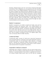
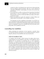
of data about the center point of all data. Figure 7.1 uses the data
just noted to determine the standard deviation, the mean, and the
coefficient of variation.
The calculations in Figure 7.1 reveal that the set of projections
used as underlying data vary significantly from the midpoint of the
group, especially in a downward direction, indicating that there is a
high degree of risk that the expected outcome will not be achieved.
Sometimes the management team to whom risk information is
reported will not be awed by a reported coefficient of variation of a
whopping 80 percent or by a standard deviation of 800 units. They
do not know what these measures mean, and they do not have time
to find out. For them, a graphical representation of data dispersion
SECTION
III
212
FIGURE 7.1
Calculating the Standard Deviation
and Coefficient of Variation
1. The standard deviation formula in Excel, using data set, is:
= STDEV(250, 400, 675, 725, 850, 875)
= 252
2. The calculation of the mean of all data is:
= (sum of all data items)/(number of data items)
= (250 + 400 + 675 + 725 + 850 + 875)/6
= 629

3. The calculation of the coefficient of variation is:
= (standard deviation)/(mean)
= 252/629
= 40%
p03.qxd 11/29/05 8:45 AM Page 212
may be a better approach. They can see the spread of estimates on
a graph and then decide for themselves if there appears to be a
problem with risk.
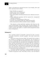
When constructing a graph that shows the dispersion of data,
you can lay out the data set in terms of the percentage difference
between each item and the midpoint. Figure 7.2 takes the projec-
tion information used in Figure 7.1 and converts it into percentages
from the median.
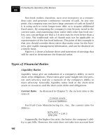
When translated into a graph, Figure 7.2 gives a wide percent-
age distribution of data on either side of the X axis that gives a good
indication of the true distribution of data about the mean. The top
graph of Figure 7.3 restates the data in Figure 7.2.
Note that there are two additional graphs in Figure 7.3. The
middle graph assumes that there are a number of projections clus-
tered under each of the variance points. The example arbitrarily
expands the number of projections to 26, with 8 clustered at the
median point, 6 each at the −4% and +4% variance points, and
lesser amounts at the outlying variance points. This is close to a clas-
sic “bell curve” distribution, where the bulk of estimates are clus-
tered near the middle and a rapidly declining number are located at
the periphery. This is an excellent way to present information, but
small business owners rarely have a sufficient number of projec-
tions to use this type of graph. If there are enough projections, a
variation shown in the graph at the bottom of the exhibit may
result: Data are skewed toward the right-hand side of the chart.

Financial Analysis
CHAPTER
7
213
FIGURE 7.2
Data Dispersion, Measured in Percentages
Percentage Variance
Projection from the Median
$250 −64%
$400 −43%
$675 −4%
$700 (median) 0%
$725 4%
$850 21%
$875 25%
p03.qxd 11/29/05 8:45 AM Page 213
Evaluating the Operations of the Business
SECTION
III
214
FIGURE 7.3
Graphical Illustration of Data Dispersion
Percent Distribution from Median
-64%
-43%
0%
21%
25%
-80%
-60%

-40%
-20%
0%
20%
40%
012345678
Dispersion by No. of Data Items
21%
4%
0%
-4%
-64%
25%
-43%
-2
0
2
4
6
8
10
Positive Skew in Data Items
-64%
-43%
-4%
0%
4%
21%
25%
-2

0
2
4
6
8
10
p03.qxd 11/28/05 1:39 PM Page 214
This indicates a preponderance of estimates that lean, or “skew,”
toward the higher end of the range of estimates. A reverse graph,
which had negative skew, would present a decided lean toward the
left side.
Of the graphs presented in Figure 7.3, only the first one, the
“Percent Distribution from Median,” is likely to be used consistently,
because in most situations there are so few data points available to
work with. Nonetheless, you can use any of these graphs when
making presentations to management about the riskiness of projec-
tions, because they all are so easy to understand.
Capacity Utilization
The term capacity covers both human and machine resources. If
those resources are not used to a sufficient degree, there are imme-
diate grounds for eliminating them, either by a layoff (in the case of
human capacity) or selling equipment (in the case of machines). A
layoff usually has a short-term loss associated with it, which covers
severance costs, followed by an upturn in profits, since there is no
longer a long-term obligation to pay salaries. The sale of a machine
does not have much of an impact on profits, unless there is a gain
or loss on sale of the asset, but it will result in an improvement in
cash flow as sale proceeds come in; these funds can be used for a
variety of purposes to increase corporate value, such as reinvest-
ment in new machines, a loan payoff, a buyback of equity, and so

on. Consequently, you should keep a close eye on capacity levels
throughout a company. Whoever makes recommendations to keep
capacity utilization close to current capacity levels will have a sig-
nificant impact on both profits and cash flows.
When making such analyses, an issue to be aware of is that a
business owner tends to be conservative—he or she wants to max-
imize the use of current capacity and get rid of everything not being
used. This may not be a good thing when activity levels are pro-
jected to increase markedly in the near term. If management elim-
inates excess capacity just prior to a large increase in production
volumes, some exceptional scrambling, possibly at high cost, will be
required to bring the newly necessary capacity back in house.
Financial Analysis
CHAPTER
7
215
p03.qxd 11/28/05 1:39 PM Page 215
Evaluating the Operations of the Business
Consequently, be sure to work with the sales staff to determine
future sales (and therefore production) trends before recommend-
ing any cuts in capacity.
Capacity utilization also reveals the specific spots in a produc-
tion process where work is being held up. These bottleneck oper-
ations prevent a production line from attaining its true potential
amount of revenue production. You can use this bottleneck infor-
mation in two ways:
1. To recommend improvements to bottleneck operations in order
to increase the potential amount of revenue generation
2. To point out that any capital improvements to other segments of
a production operation are essentially a waste of money (from

the perspective of increasing the flow of production), since all
production still is going to create a log-jam in front of the bot-
tleneck operation
Another use for capacity utilization information is in the deter-
mination of pricing levels. For example, if a company has a large
amount of surplus excess capacity and does not intend to sell it off
in the near term, it makes sense (and cents) to offer pricing deals on
incremental sales that result in only small margins. This is because
there is no other use for the equipment or production personnel. If
low-margin jobs are not produced, the only alternative is no jobs at
all, for which there is no margin at all. However, if the business
owner knows that a production facility is running at maximum
capacity, it is time to be choosy on incremental sales, so that only
those sales involving large margins are accepted. It may also be pos-
sible to stop taking orders for low-margin products in the future,
thereby flushing such products out of the current production mix
in favor of newer, higher-margin sales. Although this approach is
highly profitable, it can irritate customers who are faced with take-
it-or-leave-it answers by a company that refuses new orders unless
the customer accepts higher prices. Consequently, incremental
pricing for new sales is closely tied not only to how much produc-
tion capacity a company has left, but also to its long-term strategy
for how it wants to treat its customers.
Companies have a variety of activities in which the capacity
SECTION
III
216
p03.qxd 11/28/05 1:39 PM Page 216
utilization may be important enough to track. The area most com-
monly measured is machine utilization, because management teams

are always interested in keeping expensive machinery running for
as long as possible, so that the invested cost is not wasted. Thus,
capacity tracking for expensive assets is certainly a common activity.
However, another factor that many organizations miss is the
capacity utilization measurement for any bottleneck operation. This
has nothing to do with a costly asset, but rather with determining
whether a key operation in a process is interfering with the suc-
cessful processing of a transaction. For example, if a number of pro-
duction lines feed their products to a single person who must box
and ship them, and this person cannot keep up with the volume of
production arriving at her workstation, then she is a bottleneck
operation that is interfering with the timely completion of the
production schedule. Because she is a bottleneck, her capacity uti-
lization should be tracked most carefully. This worker is not an
expensive machine, and may in fact be paid very little, but she is
potentially holding up the realization of a great deal of revenue that
cannot be shipped to customers. Consequently, using a capacity
utilization measure makes a great deal of sense in this situation.
To amplify on the concept of capacity planning for bottleneck
operations, it is not sufficient to track the utilization of a single bot-
tleneck operation, because the bottleneck will move to different
steps in the production process as improvements are made to the
system. For example, the key principle of the just-in-time concept
is that management works to identify bottleneck operations and fix
them. As a result, each specific bottleneck will be eliminated, but
now the second most constrictive operation comes to the fore for
review and improvement, which in turn will be followed by a third
operation, and so on. Consequently, it is better to identify every work
center and track the utilization of them all. By using this more com-
prehensive approach, management can spot upcoming bottleneck

problems and address them before they become serious problems.
In the case of machinery, the tracking of utilization for virtually
all of them is also useful, not just because they are also potential bot-
tleneck operations, but because of the reverse problem—a machine
that is not being used is a waste of invested capital and should be
sold off if possible. A detailed capacity utilization report will note
Financial Analysis
CHAPTER
7
217
p03.qxd 11/28/05 1:39 PM Page 217
Evaluating the Operations of the Business
those machines that are not being used and tell management what
can potentially be eliminated. This information is especially useful
when machines are clustered on the report by type, so that a subto-
tal of capacity utilization is noted for each group of machines. If the
machines within each cluster can be used interchangeably to com-
plete similar work, management can determine the total amount of
work required of each cluster and add or delete machines to meet
that demand, which results in a very efficient use of capital. Such a
report is described later in Figure 7.4.
A company frequently thinks of its production capacity only in
terms of the current number of shifts being operated, and tracks its
capacity utilization accordingly. For example, a production facility
that operates for one eight-hour shift and uses all machinery dur-
ing that time thinks that it is operating at 100 percent capacity uti-
lization. In fact, it is only using one-third of the available hours in a
day, which leaves lots of room for additional production. Accord-
ingly, when developing a utilization measurement, always use the
maximum amount of theoretical capacity as the baseline, rather than

the amount of time during the day that is currently being used. For
a single day, this means 24 hours, and for a week, it is 168 hours.
On a monthly basis, the total number of hours will vary, since the
number of days in a month can vary from 28 to 31. To get around
this problem, it is easier to track capacity on a weekly basis and use
either four or five full weeks for individual months, depending on
where the final month-end dates fall, so that all months of the year
(except the last) on the capacity report show full-week results for
either four or five weeks.
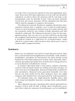
Once the decision is made to create a capacity utilization analy-
sis, what format should be used to present it? The capacity report in
Figure 7.4 lists the utilization hours of 28 plastic injection and blow
molding machines. The identification number of each machine is
listed down the left column, with the tonnage of each machine
noted in the next column. The next cluster of four columns shows
the weekly utilization in hours for each machine. The final three
columns show the average weekly utilization by machine for the
preceding three months. In addition, there are subtotals for all
blow molding machines and for five clusters of injection molding
machines, grouped by tonnage size.
SECTION
III
218
p03.qxd 11/28/05 1:39 PM Page 218
219
FIGURE 7.4
Capacity Utilization Report
Month of
Machine Machine 5/9–5/15 5/2–5/8 Apr. Mar. Feb.
ID Description Run Hrs Run Hrs Run Hrs Run Hrs Run Hrs Run Hrs Run Hrs

B1100/BM04 Blow Mold 150 142 139 132 112 122 104
B2000/BM03 Blow Mold 149 135 137 152 114 154 119
89% 82% 82% 85% 67% 82% 66%
01-25 25 Ton 123 125 126 132 138 125 111
02-90/TO11 90 Ton 150 158 152 137 117 132 144
03-90/TO10 90 Ton 129 168 164 129 126 111 120
04-90/TO09 90 Ton 75 50 94 138 142 167 147
16-55/AG01 55 Ton 132 168 163 59 125 109 102
73% 80% 83% 71% 61% 62% 61%
05-150/TO08 150 Ton 141 150 147 162 133 139 133
06-150/TO07 150 Ton 119 130 137 152 122 124 127
07-198/TO06 198 Ton 147 135 133 77 114 132 54
08-200/TO05 200 Ton 110 120 124 141 117 101 113
17-190/TA05 190 Ton 138 141 127 116 97 106 91
78% 80% 80% 77% 69% 72% 62%
09-300/TO04 300 Ton 168 168 168 133 148 125 148
10-300/TO03 300 Ton 0 50 79 143 135 142 129
11-330/TO02 330 Ton 148 149 129 136 93 125 100
20-390/TA04 390 Ton 110 127 121 158 128 136 154
21-375/C106 375 Ton 92 100 102 84 78 77 102
26-400/TO01 400 Ton 47 85 124 116 101 78 120
56% 67% 72% 76% 68% 68% 75%
12-500/CI05 500 Ton 91 168 166 137 113 62 50
14-500/CI04 500 Ton 74 85 100 96 107 142 96
18-450/VN02 450 Ton 168 162 163 164 103 111 119
24-500/VN01 500 Ton 125 0 167 163 161 96 106
25-500/TA03 500 Ton 132 139 145 162 146 128 89
70% 66% 88% 86% 75% 64% 55%
13-700/CI03 700 Ton 168 151 146 142 106 78 60
15-700/VN03 700 Ton 0 153 107 152 133 118 118

19-720/TA02 720 Ton 102 109 115 161 115 58 113
22-700/CI01 700 Ton 111 59 74 154 74 76 144
23-950/TA01 950 Ton 104 168 126 159 110 91 112
58% 76% 68% 91% 64% 50% 65%
66% 74% 78% 80% 71% 66% 66%
68% 74% 78% 81% 70% 67% 66%
p03.qxd 11/28/05 1:39 PM Page 219
Evaluating the Operations of the Business
This report format allows management to look across the report
from left to right and determine any trends in capacity utilization,
while also being able to look down the page and determine usage
by clusters of machines. This second factor is of extreme impor-
tance in the molding business, because each machine is very
expensive and must be eliminated if it is not being used to a suffi-
cient degree. For example, look at the tonnage range of 300–400
tons, located midway through the report. A cluster of six machines
is consistently showing between 68% and 76% percent of usage. Is
it possible to eliminate one machine, thereby spreading the work
over fewer machines and raising the overall usage percentage for
all the machines? To determine the answer using data for the high-
est utilization reporting period, which is for the first week of May,
at 76%, add up all the reported hours of usage for that cluster of
machines, which is 770, and divide the total number of hours that
the machine cluster has available, assuming that one machine has
been removed. The total number of hours available for production
will be 168 (which is seven days multiplied by 24 hours per day)
times five machines, which is 840. The result is a utilization of 92
percent for the maximum amount of work that has appeared in the
last quarter of a year. Consequently, the answer is that it is theoret-
ically possible to remove one machine from the 300–400 ton range

of machines and still be able to complete all work.
However, when using a capacity report to arrive at such conclu-
sions, there are several additional factors to consider. One is the
reliability of the machines. If they have a history of failures, then a
standard number of hours per operating period for repair work
must be factored into the utilization formula, which will reduce the
theoretical capacity of the machine. Another problem is that a
machine usually is eliminated in order to realize a cash inflow from
sale of the machine; but what if the machines most likely to be sold
will fetch only a minor amount in the marketplace? If so, it may
make more sense to retain equipment, even if unused, so that it
can take on additional work in the event of an increase in sales vol-
ume. Yet another issue is that there may be some difficulty in obtain-
ing a sufficient number of staff to maintain or run a machine during
all theoretical operating hours. For example, it is common for those
organizations with a reduced number of maintenance personnel to
SECTION
III
220
p03.qxd 11/28/05 1:39 PM Page 220
cluster those staff on the day shift for maximum efficiency, which
means that any machine failures during other hours will result in a
shut-down machine until the maintenance staff arrives the next
day. Finally, the example shows management taking actual capac-
ity utilization of its machinery to 92 percent. Is this wise, if man-
agement has essentially removed all remaining available capacity
by selling off the excess machine? What if an existing customer
suddenly increases an order and finds that the company cannot
accommodate the work, because all machines are booked? Not
only lost revenues will result, but perhaps even a lost customer.

One way in which a capacity analysis can be skewed is if there
are either a large number of small jobs running through a process,
each of which requires a small amount of downtime to switch over
to the new job, or a small number of jobs that require a very lengthy
changeover process. In either case, the amount of reported capacity
will never reach 100 percent, for the required setup time will take
up the amount of capacity that is supposedly available. One action
that management can take to alleviate this problem is to work on
reducing the changeover time needed to switch to a new job. Doing
this typically involves videotaping the changeover process and then
reviewing the tape with the changeover team to identify and imple-
ment process alterations that will result in reduced setup times.
A revenue-related problem that arises when setup times eat up
a large portion of total capacity is that the sales department may
promise customers that work will begin very soon on their orders,
because the capacity utilization report appears to reveal that there
is lots of excess capacity. When excessive changeover times do not
leave any time for additional customer orders, customers may take
their business elsewhere. To counteract this problem, it is necessary
to determine the amount of practical capacity, which is the total
capacity less the average amount of changeover time. If the setup
reduction effort noted in the preceding paragraph is implemented,
the practical capacity number will increase, because the time avail-
able for production will increase as changeover times go down.
Consequently, a review of the practical capacity should be made
fairly often to ensure that the correct figure is used.
A problem with using practical capacity as the standard measure
of how much work still can be loaded into the production system
Financial Analysis
CHAPTER

7
221
p03.qxd 11/28/05 1:39 PM Page 221
Evaluating the Operations of the Business
is that it is based on an average of actual capacity information over
several weeks or months. However, if there are one or more jobs
scheduled for a changeover that require inordinate amounts of
time to complete, the reported practical capacity measure will not
reflect reality. Similarly, if the actual changeover times are quite
small, the true capacity will be higher than the reported practical
capacity. Because practical capacity is a historical average, the actual
capacity will be somewhat higher or lower than this average nearly
all of the time. Although a company with a lot of excess capacity
might call this hair-splitting, a company that is running at maximum
production levels may find itself blindsided by a lack of available
time or some amount of unplanned downtime. In either case, there
is a cost to having inaccurate capacity information. Those companies
with well-maintained manufacturing resources planning software
can avoid this problem by accurately scheduling jobs and changeover
times, and updating the data as soon as changes are made.
Breakeven Analysis
A company usually operates within a very narrow band of pricing
and costs in order to earn a profit. If it does not charge a minimum
price to cover its fixed and variable costs, it will quickly burn
through its cash reserves and go out of business. In a competitive
environment, prices drop to the point where they only barely cover
costs, and profits are thin or nonexistent. At this point, only those
companies with a good understanding of their own breakeven
points and those of their competitors are likely to make the correct
pricing and cost decisions to remain competitive. This section shows

how breakeven (also known as the cost-volume-profit relationship)
is calculated, as well as a variety of more complex variations on the
basic formula.
The breakeven formula is an exceedingly simple one. To deter-
mine a breakeven point, add up all the fixed costs for the company
or product being analyzed, and divide it by the associated gross mar-
gin percentage. This results in the sales level at which a company
will neither lose nor make money—its breakeven point. The for-
mula is shown in Figure 7.5.
SECTION
III
222
p03.qxd 11/28/05 1:39 PM Page 222
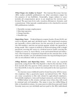
For those who prefer a graphical layout to a mathematical for-
mula, a breakeven chart can be quite informative. In the sample
chart shown in Figure 7.6, the horizontal line across the chart rep-
resents the fixed costs that must be covered by gross margins, irre-
spective of the sales level. The fixed-cost level will fluctuate over
time and in conjunction with extreme changes in sales volume, but
we will assume no changes for the purposes of this simplified analy-
sis. Also, an upward-sloping line begins at the left end of the fixed-
cost line and extends to the right across the chart. This is the
percentage of variable costs, such as direct labor and materials, that
are needed to create the product. The last major component of the
chart is the sales line, which is based in the lower left corner of the
chart and extends to the upper right corner. The amount of the sales
volume in dollars is noted on the vertical axis, while the amount of
production capacity used to create the sales volume is noted across
the horizontal axis. Finally, a line that extends from the marked
breakeven point to the right, which is always between the sales line

and the variable cost line, represents income tax costs. These are
the main components of the breakeven chart.
It is also useful to look between the lines on the graph and
understand what the volumes represent. For example, as noted in
Figure 7.6, the area beneath the fixed-cost line is the total fixed cost
to be covered by product margins. The area between the fixed-cost
line and the variable-cost line is the total variable cost at different
volume levels. The area beneath the income line and above the vari-
able cost line is the income tax expense at various sales levels.
Finally, the area beneath the revenue line and above the income tax
line is the amount of net profit to be expected at various sales levels.
Although this breakeven chart appears quite simplistic, addi-
tional variables can make a real-world breakeven analysis a much
more complex endeavor to understand. One of these variables is
fixed cost. A fixed cost is a misnomer, for any cost can vary over
Financial Analysis
CHAPTER
7
223
FIGURE 7.5
The Breakeven Formula
Total Fixed Costs/Gross Margin Percentage = Breakeven Sales Level
p03.qxd 11/28/05 1:39 PM Page 223
Evaluating the Operations of the Business
time, or outside of a specified set of operating conditions. For exam-
ple, the overhead costs associated with a team of engineers may be
considered a fixed cost if a product line requires continuing improve-
ments and enhancements over time. However, what if manage-
ment decides to gradually eliminate a product line and milk it for
cash flow, rather than keep the features and styling up-to-date? If

so, the engineers are no longer needed, and the associated fixed
cost goes down. Any situation where management is essentially
abandoning a product line in the long term probably will result in a
decline in overhead costs.
A much more common alteration in fixed costs is when additional
SECTION
III
224
FIGURE 7.6
Simplified Breakeven Chart
euneveR
50%
0% 100%
Percenta
g
e of Production Utilization
stsoC

elb
airaV
Breakeven Point
s
e
x
aT emocnI
emuloV
selaS
Fixed
Costs
Variable

Costs
Income
Taxes
Net
Profit
p03.qxd 11/28/05 1:39 PM Page 224
personnel or equipment are needed in order to support an increased
level of sales activity. As noted in the breakeven chart in Figure 7.7,
the fixed cost will step up to a higher level (an occurrence known as
step costing) when a certain capacity level is reached. An example
of this situation is when a company has maximized the use of a sin-
gle shift and must add supervision and other overhead costs, such
as electricity and natural gas expenses, in order to run an additional
shift. Another example is when a new facility must be brought on
line or an additional machine acquired. Whenever this happens,
management must take a close look at the amount of fixed costs
that will be incurred, because the net profit level may be less after
the fixed costs are added, despite the extra sales volume. In the fig-
ure, the maximum amount of profit that a company can attain is at
the sales level just prior to incurring extra fixed costs, because the
increase in fixed costs is so high. Although step costing does not
always involve such a large increase in costs as noted in the next
exhibit, this is certainly a major point to be aware of when increas-
ing capacity to take on additional sales volume. In short, more sales
do not necessarily lead to more profits.
The next variable in the breakeven formula is the variable cost
line. Although you would think that the variable cost is a simple
percentage that is composed of labor and material costs, and which
never varies, this is not the case. This percentage can vary consid-
erably and frequently drops as the sales volume increases. The rea-

son for the change is that the purchasing department can cut better
deals with suppliers when it orders in larger volumes. In addition,
full truckload or railcar deliveries result in lower freight expenses
than would be the case if only small quantities were purchased.
The result is shown in Figure 7.8, where the variable cost percent-
age is at its highest when sales volume is at its lowest and gradually
decreases in concert with an increase in volume.
Because material and freight costs tend to drop as volume
increases, it is apparent that profits will increase at an increasing
rate as sales volume goes up, although there may be step costing
problems at higher capacity levels.
Another point is that the percentage of variable costs will not
decline at a steady rate. Instead, and as noted in Figure 7.8, there will
Financial Analysis
CHAPTER
7
225
p03.qxd 11/28/05 1:39 PM Page 225
Evaluating the Operations of the Business
be specific volume levels at which costs will drop. This is because the
purchasing staff can negotiate price reductions only at specific vol-
ume points. Once such a price reduction has been achieved, there
will not be another opportunity to reduce prices further until a sep-
arate and distinct volume level is reached once again.
The changes to fixed costs and variable costs in the breakeven
analysis are relatively simple and predictable, but now we come to
the final variable, sales volume, which can alter for several reasons,
making it the most difficult of the three components to predict.
The first reason why the volume line in the breakeven chart can
vary is the mix of products sold. A perfectly straight sale volume

SECTION
III
226
FIGURE 7.7
Breakeven Chart Including Impact of Step Costing
eun
eveR
50%
0% 100%
Percentage of Production Utilization
Breakeven Point
s
exaT e
mocn
I
emuloV

selaS
Fixed
Costs
Variable
Costs
Income
Taxes
Net
Profit
s
t
soC


e
lba
iraV
e
u
neve
R
p03.qxd 11/28/05 1:39 PM Page 226
line, progressing from the lower left to the upper right corners of
the chart, assumes that the exact same mix of products will be sold
at all volume levels. Unfortunately, it is a rare situation indeed
where this happens, because one product is bound to become more
popular with customers, resulting in greater sales and variation in
the overall product mix. If the margins for the different products
being sold are different, then any change in the product mix will
result in a variation, either up or down, in the sales volume achieved,
which can have either a positive or negative impact on the result-
ing profits. As it is very difficult to predict how the mix of products
sold will vary at different volume levels, most company owners do
Financial Analysis
CHAPTER
7
227
FIGURE 7.8
Breakeven Chart Including Impact of Volume Purchases
e
un
ev
eR
50%

0% 100%
Percentage of Production Utilization
Breakeven Point
emuloV selaS
Fixed
Costs
Variable
Costs
Income
Taxes
Net
Profit
e
u
n
ev
eR
s
tsoC
e
l
bairaV
s
e
xa
T

e
mo
cn

I
Most Expensive
Level of
Variable Costs
Least Expensive
Level of
Variable Costs
p03.qxd 11/28/05 1:39 PM Page 227
Evaluating the Operations of the Business
not attempt to alter the mix in their projections, thereby accepting
the risk that some variation in mix can occur.
The more common problem that impacts the volume line in the
breakeven calculation is that unit prices do not remain the same
when volume increases. Instead, a company finds that it can charge
a high price early on, when the product is new and competes with
few other products in a small niche market. Later, when manage-
ment decides to go after larger unit volume, unit prices drop in
order to secure sales to a larger array of customers or to resellers
who have a choice of competing products to resell. For example,
the price of a personal computer used to hover around $3,000 and
was affordable for less than 10 percent of all households. As of this
writing, the price of a personal computer has dropped to as little as
$400, resulting in more than 50 percent of all households owning
one. Thus, higher volume translates into lower unit prices. The
result appears in Figure 7.9, where the revenue per unit gradually
declines despite a continuing rise in unit volume, which causes a
much slower increase in profits than would be the case if revenues
rose in a straight, unaltered line.
The breakeven chart in Figure 7.9 may make management
think twice before pursuing a high-volume sales strategy, since

profits will not necessarily increase. The only way to be sure of
the size of price discounts would be to begin negotiations with
resellers or to sell the product in test markets at a range of lower
prices to determine changes in volume. Otherwise, management
is operating in a vacuum of relevant data. Also, in some cases the
only way to survive is to keep cutting prices in pursuit of greater
volume, because there are no high-priced market niches in which
to sell.
The chart in Figure 7.9 is a good example of what the breakeven
analysis really looks like in the marketplace. Fixed costs jump at
different capacity levels, variable costs decline at various volume
levels, and unit prices drop with increases in volume. Given the flu-
idity of the model, it is reasonable to revisit it periodically in light of
continuing changes in the marketplace in order to update assump-
tions and make better calculations of breakeven points and pro-
jected profit levels.
SECTION
III
228
p03.qxd 11/28/05 1:39 PM Page 228
Summary
From a practical perspective, you should use capacity analysis reg-
ularly. Doing so can involve the monitoring of: revenue per person,
usage levels of various machines, sales per salesperson, or the need
for requested capital purchases. All of these issues involve changes
in staffing or machinery, which are exceedingly expensive. Accord-
ingly, regularly verify that the organization does not expend too
much for excess capacity, instead keeping capacity levels at the
highest possible level while ensuring that there is some excess
capacity available for short-term growth.

Financial Analysis
CHAPTER
7
229
FIGURE 7.9
Breakeven Chart Including Impact of Variable Pricing Levels
50%
0% 100%
Percentage of Production Utilization
Breakeven Point
emuloV
sela
S
Fixed
Costs
Variable
Costs
Income
Taxes
Net
Profit
Most Expensive
Level of
Variable Costs
Least Expensive
Level of
Variable Costs
Highest Price
Per Unit
Lowest Price

Per Unit
e
u
ne
v
e
R
stsoC elbairaV
sexaT emoc
n
I
eunev
eR
Fixed Costs
sex
a
T
emocnI
p03.qxd 11/28/05 1:39 PM Page 229
Evaluating the Operations of the Business
Breakeven analysis should be a required part of any proposal to
alter the underlying structure of a business. By reviewing it, you
can tell if any alterations, such as to price points, capital expendi-
tures, or the incurrence of new expenses, will have a significant
impact on the ability of the organization to exceed its breakeven
point on a regular basis.
SECTION
III
230
p03.qxd 11/28/05 1:39 PM Page 230

Chapter
8
Taxes and Risk
Management
M
any of the tax consequences to a firm are covered in Chap-
ter 9, “Reporting.” This chapter points out how to manage
taxes on a continuous basis in order to take advantage of the bene-
fits associated with various liability-limiting provisions in the tax
code. Without consideration on an ongoing basis, taxes can become
a significant drain on the business’s cash flow.
If you consider that under the federal corporate tax rates, one
of the largest percentage deductions from a company’s profits may
come as payment of taxes on an annual basis, you quickly realize
that significant gains can be made if taxes can be deferred or, bet-
ter still, eliminated. There are many tax choices available to busi-
nesspeople that may eliminate or defer payment of income taxes.
Although very few situations permit the permanent deferral of
taxes, the law permits temporary deferral of tax payments in cer-
tain situations. Such tax deferral has these benefits:
• Deferring taxes lowers a company’s cash flow commitment to
the government. This means more cash will be available for
withdrawal and use for profit-making opportunities.
• If taxes can be deferred long enough, there is a chance that the
federal government will change the tax code to make the pay-
ment of taxes more favorable or eliminate some tax liability
231
p03.qxd 11/28/05 1:39 PM Page 231