2 Wireless Mesh Networks
to the reliability aspect of such networks. In this chapter, we propose an analytical model
for apparent link-failures in static mesh networks where the location of each node is carefully
planned (referred to hereafter as planned mesh network). A planned mesh network typically
appears as a consequence of the high costs associated with interconnecting nodes in a network
with wired links. For example, ad hoc technology can in a cost-efficient manner, extend the
reach of a wired backbone through a wireless backhaul mesh network. Apparent link-failures
are often a significant cause for performance degradation of mesh networks, and thus a model
is needed in order to diminish their effect. For instance, with a model in place it is possible to
detect and avoid undesirable topologies that might lead to a high frequency of such failures.
The proposed model makes use of the assumption that the probability of losing a beacon
due to a packet collision with transmissions from hidden nodes (p
e
), is much larger than
the probability of losing beacons due to transmissions from one-hop neighbors (p
col l
). The
probability that a receiving node considers a link to be inoperative at the time a beacon
is expected, is then estimated through analysis using a Markov model. Furthermore, an
algorithm which is used for determining the number of hidden nodes and the associated
traffic pattern is introduced so that the model can be applied to arbitrary topologies.
1.2 Significance of our results
By avoiding poorly planned topologies, not only the reliability of mesh networks can
be increased, but also the general performance of such networks can be improved.
Apparent link-failures are often a significant cause for performance degradation of ad hoc
networks since erroneous routing information may be spread in the network when apparent
link-failures happen. Also, it might lead to a disconnected topology or less optimal routes to
a destination. Analysis of a real life network Li et al. (2010) has demonstrated that it takes a
significant amount of time to restore failed links Egeland & Li (2007). An example of the effect
of these failures is illustrated in Fig. 1. Using a well known network simulator ns2 (2010)
we have measured the throughput from node d

8
→d
7
in the topology shown in Fig. 1(a).
As the load from the hidden nodes increases, the throughput from node d
8
→d
7
is reduced,
because the routing protocol forces the data packets to traverse longer paths in order to bypass
the apparent link-failure or simply because node d
7
drops packets when buffers are filled as
a result of having no operational route to node d
8
. The throughput would remain relatively
stable if the apparent link-failures were eliminated, as seen from the ”No apparent link failure”
graph in Fig. 1(b).
The model presented in this chapter allows a node to calculate the probability of losing
connectivity to its one-hop neighbors caused by beacon loss. Utilizing the model, we
demonstrate how a node in a mesh network operated on the Optimized Link State Routing
(OLSR) Clausen & Jacquet (2003) routing protocol can apply the apparent link-failure
probability as a criterion to decide when to unicast and when to broadcast beacons to
surrounding neighbors, thus improving the packet delivery capability.
1.3 Related work
In Voorhaen & Blondia (2006) the performance of neighbour sensing in ad hoc networks is
studied, however, only parameters such as the transmission frequency of the Hello-messages
and the link-layer feedback are covered. In Ray et al. (2005) a model for packet collision and
the effect of hidden and masked nodes are studied, but only for simple topologies, and the
work is not directly applicable to the Hello-message problem. The work in Ng & Liew (2004)

addresses link-failures in wireless ad hoc networks through the effect of routing instability.
164
Wireless Mesh Networks
The Performance of WirelessyMesh Networks with Apparent Link Failures 3
d
0
d
1
d
2
d
3
d
4
d
5
d
6
d
7
d
8
d
9
d
10
d
11
d
12

(a) Example topology
0.00 0.05 0.10 0.15 0.20 0.25
Load from hidden nodes {d
4
,d
10
,d
12
} (λ
c
T )
0.01
0.02
0.03
0.04
0.05
0.06
Throughput as fraction of channel capacity (d
8
→ d
7
)
Fixed rate (d
8
→ d
7
) with no apparent link-failures.
Fixed rate
(d
8

→ d
7
) with
apparent link-failures.
Apparent link-failures
No apparent link-failures
(b) Throughput from node d
8
→ d
7
Fig. 1. Performance with and without apparent link-failures. The possibility of apparent link
failures is artificially removed by not allowing the links to time out when beacons are lost.
Here the authors study the throughput of TCP/UDP in networks where the routing protocol
falsely assumes a link is inoperable. However, what causes a link to become unavailable to
the routing protocol is not studied. A model for packet collision and the effect of hidden
and masked nodes are studied in Ray et al. (2004), but only for simple topologies, and
the work is not directly applicable to loss of beacons. Not much published work relates
directly to the modeling of apparent link-failures caused by loss of beacons. In Egeland &
Engelstad (2009) the reliability and availability of a set of mesh topologies are studied using
both a distance-dependent and a distance-independent link-existence model, but the effects
of beacon-based link maintenance and hidden nodes are ignored. Here it is assumed that
apparent link-failures are a result of radio-induced interference only. The work in Gerharz
et al. (2002) studies the reliability of wireless multi-hop networks with the assumptions that
link-failures are caused by radio interference.
2. Network model
2.1 Network terminology
This chapter reuses the terminology of wireless mesh networks in order to describe the
architecture of a planned mesh network, more specifically of the IEEE 802.11s specification
IEEE802.11s (2010) of mesh networks. In this terminology a node in a mesh network is referred
to as a Mesh Point (MP). Furthermore, an MP is referred to as a Mesh Access Point (MAP) if it

includes the functionality of an 802.11 access point, allowing regular 802.11 Stations (STAs)
access to the mesh infrastructure. When an MP has additional functionality for connecting
the mesh network to other network infrastructures, it is referred to as a Mesh Portal (MPP). A
mesh network is illustrated in Fig. 2.
A mesh network can be described as a graph G
(V,E) where the nodes in the network serve
as the vertices v
j
∈V(G). Any two distinct nodes v
j
and v
i
create an edge 
i,j
∈E(G) if
there is a direct link between them. In order to provide an adequate measure of network
reliability, the use of probabilistic reliability metrics and a probabilistic graph is necessary.
This is an undirectional graph where each node has an associated probability of being in an
operational state, and similarly for each edge, i.e. the random graph G
(V,E, p) where p is
165
The Performance of Wireless Mesh Networks with Apparent Link Failures
4 Wireless Mesh Networks
Wired infrastructure
MPP
MP MP
MP
MP: Mesh Point
MPP: Mesh Portal
MAP: Mesh Access Point

STA: Station
MAP MAP
STA
1
STA
2
STA
3
STA
4
STA
5
Fig. 2. A wireless mesh network connected to a fixed infrastructure.
the link-existence probability. An underlying assumption in the analysis is that the existence
of a link is determined independently for each link. This means that the link 
s,d
may fail
independently of the link 
i,j
∈E(G) \{
s,d
}. As the link failure probability in general is much
higher than the node failure probability, it is natural to model the nodes v
j
∈V(G) in the
topology as invulnerable to failures. Thus, a mesh network can be described and analyzed
as a random graph.
2.2 Link maintenance using beacons
In a multi-hop network, links are usually established and maintained proactively by the use of
one-hop beacons which are exchanged between neighboring nodes periodically. Beacons are

broadcast in order to conserve bandwidth, as no acknowledge messages are expected from the
receivers of these beacons. Thus, the link status of every link on which a beacon is received
can be effectively obtained through beacon transmissions. Since broadcast packets are not
acknowledged, beacons are inherently unreliable. A node anticipates to receive a beacon from
a neighbor node within a defined time interval and can tolerate that beacons occasionally
will be missing due to various error events like channel fading or packet collision. However, a
node failed to receive a number of (θ
+1) consecutive beacons will accredit that the node on the
other side of the link is permanently unreachable and that the link is inoperable. The value
of the configurable parameter θ is a tradeoff between providing the routing protocol with
stable and reliability links (a large θ), and the ability to detect link-failures in a timely and
fast manner (a small θ). Since beacons are broadcast, they are unable to take the advantage of
the Request-To-Send/Clear-To-Send (RTS/CTS) signaling that protects the IEEE 802.11 MAC
protocol’s IEEE802.11 (1997) unicast data transmission against hidden nodes. Although some
beacon loss is avoided using RTS/CTS for the unicast data traffic in the network, it will only
affect the links of the node that issues the CTS. The consequence is that beacons will be
susceptible to collisions with traffic from hidden nodes even if RTS/CTS is enabled. Thus, the
utilization of a link may be prevented if the link is assumed to be inoperable due to beacon
loss. Examples of routing protocols that make use of beacons are the proactive protocol OLSR
Clausen & Jacquet (2003) and an optional mode of operation for the reactive Ad hoc On-Demand
Distance Vector (AODV) routing protocol Perkins et al. (2003).
A major difference between various beacon-based schemes is how the routing protocol
determines if a failed link is operational again. Stable links are desirable, and introducing
a link too early can lead to a situation where a link oscillates between an operational
and a non-operational state. A solution that avoids this situation is by measuring the
Signal-to-Noise Ratio (SNR) of the failed link and define the link as operational only when
166
Wireless Mesh Networks
The Performance of WirelessyMesh Networks with Apparent Link Failures 5
s

0
s
2
s
1
s
6
s
4
s
3
s
5
s
7
B
D
D
D
(a) Isolated hidden nodes
s
0
s
2
s
1
s
6
s
4

s
3
s
5
s
7
B
D
D
D
(b) Connected hidden nodes
Fig. 3. Sample topologies where the hidden nodes {s
2
,s
4
,s
6
} are isolated or connected. When
the hidden nodes send data (D), this may collide with the beacons (B) sent by node s
0
.
both beacons are being received and the received SNR is above a defined threshold Ali et al.
(2009). However, if SNR measurement is not available or not practical, a simple solution
is to introduce some kind of hysteresis by requiring a number of consecutive beacons to be
received (θ
h
+ 1) before the link is assumed to be operational. This is the solution chosen in
this analysis.
3. Apparent link-failures due to beacon loss
3.1 Assumptions for the beacon-based link maintenance

Before we can determine the apparent link-failure probability, a model for identifying losing
a single beacon caused by overlapping transmissions must be found. In order to simplify the
analysis, the model is based upon three assumptions. First, it is assumed that a beacon sent by
a node has a negligible probability of colliding with a beacon from any of the neighboring
nodes. This is a fair assumption, since beacons are short packets that are transmitted
periodically and at a random instant at a relatively low rate. Secondly, it is assumed that
the probability of a beacon colliding with a data transmission from any of the (non-hidden)
neighboring nodes also is negligible, i.e. p
e
p
col l
. This assumption is also fair, since a
MAC layer often has mechanisms that reduce such collisions to a minimum. Examples of
such mechanisms are the collision avoidance scheme of the IEEE 802.11 MAC protocol with
randomized access to the channel after a busy period, and the carrier- and virtual sense of
the physical layer. Accordingly to the IEEE 802.11 standard, a beacon will be deferred at
the transmitter if there is ongoing transmission on the channel. Therefore, the probability
that beacons are lost, is a result of overlapping data packet transmissions from hidden nodes only.
Thirdly, we make the assumption that the packet buffers of a node can be modeled as an
M/M/1 queue Kleinrock (1975) and that the packet arrival rate is Poisson distributed with
parameter λ
c
and that the channel access and data packet transmission times are exponential
distributed with parameter 1/μ.
These assumptions allow us to verify the model in a simple manner. Even though traffic
in a real network may follow other distributions, the results presented later in the chapter
suggest that the assumptions are fair. The bounds for beacon loss probability based on a large
number of random independent traffic scenarios will be presented, and these capture more of
the characteristics of the traffic in a real-life network.
3.2 Probability of losing a beacon p

e
Consider the topology in Fig. 3(a). We need to find firstly the probability (p
e
) that the beacon
from s
0
and a data packet from the hidden node s
2
collide. Let q
s
2
(0) denote the probability of
167
The Performance of Wireless Mesh Networks with Apparent Link Failures
6 Wireless Mesh Networks
x
0
x
1
x
2
···
x
N−1
x
N
mλ
c
mλ
c

mλ
c
mλ
c
mλ
c
μz
N
μz
N−1
μz
3
μz
2
μz
1
Fig. 4. A Markov model of the total number of packets waiting to be transmitted by the m
hidden nodes, where λ
c
is the packet arrival rate, 1/μ is the service time and z
n
is the
average number of the m hidden nodes transmitting simultaneously.
node s
2
having zero packets awaiting in its buffer. p
e
can be expressed as Dubey et al. (2008):
p
e

= Pr{Collision|q
s
2
(0) > 0} ·Pr{q
s
2
(0) > 0}
+ Pr{Collision|q
s
2
(0)=0} · Pr{q
s
2
(0)=0}
=(1 − p
0
) · 1 +(1 − e
−λ
c
ω
b
/T
p
) · p
0
(1)
where p
0
is the probability that the hidden node s
2

has zero packets awaiting to be transmitted.
The parameters T
p
and ω
b
represent the average transmission time of the data packet
and of the beacon packet, respectively. Both these transmission times are assumed to be
exponentially distributed. The probability that a node has i data packets in its packet queue is
given by p
i
=(1 − ρ)ρ
i
, where ρ = λ
c
/μ, thus p
0
= 1 −ρ Kleinrock (1975).
3.2.1 Isolated hidden nodes
We will now evaluate the probability that a beacon collides with data transmissions from a
set of hidden nodes using the topology illustrated in Fig. 3(a). In this sample topology, the
hidden nodes are assumed to be isolated, i.e. outside the transmission range of each other.
Individually, the probability that one of them sends a data packet which overlaps with a
beacon from node s
0
is given by Eq. (1) (denoted p
e
). The number of data packets from
{s
2
,s

4
,s
6
} overlapping with a beacon from s
0
is binomially distributed B(m, p
e
) where m is
the number of hidden nodes. The probability that a beacon is lost can then be expressed as:
p
I
e
=
m
∑
k=1

m
k

p
k
e
(1 − p
e
)
m−k
. (2)
3.2.2 Connected hidden nodes
In Fig. 3(b) the hidden nodes are all within radio transmission range of each other. When

all the hidden nodes are connected, the calculation of the beacon loss probability is not
as straightforward, and we need to make further simplified assumptions. Firstly, it is
assumed that the nodes access the common channel according to a 1-persistent CSMA protocol
Kleinrock & Tobagi (1975). This might seem like a contradiction, since it was stated earlier that
we assumed a MAC protocol that reduces the collisions between non-hidden neighbours to
a minimum. However, for the case where the hidden nodes are connected, there will be a
parameter ( z
n
) in the model that can be set to control to which extent transmissions between
the hidden nodes are permitted to collide with each other. Secondly, it is assumed that the
arrival rates at the different hidden nodes are not coupled, hence a Markov model can be used
for the analysis.
Consider the Markov chain illustrated in Fig. 4. Each state represents the sum of all
packets queuing up in the m hidden nodes. Here z
n
is the average number of hidden nodes
transmitting when a total of n packets are distributed amongst the hidden nodes.
168
Wireless Mesh Networks
The Performance of WirelessyMesh Networks with Apparent Link Failures 7
We are now able to find the probability of being in state x
0
, which is the case for which none
of the hidden nodes have packets awaiting transmission (p
C
0
). Using standard queuing theory
Kleinrock (1975), it can easily be shown that this probability is given by:
p
C

0
=
⎡
⎣
1
+
N
∑
i=1
(mρ)
i

i
∏
n=1
z
n,i

−1
⎤
⎦
−1
, ρ =
λ
c
μ
(3)
where z
n,i
is the average number of the m nodes transmitting simultaneously and is calculated

according to:
z
n
=
⎧
⎪
⎪
⎪
⎪
⎪
⎨
⎪
⎪
⎪
⎪
⎪
⎩
∑
n
k
=1
k
(
m
k
)(
n−1
k
−1
)(

1 − ρ
m
)
∑
n
k
=1
(
m
k
)(
n−1
k
−1
)
n<m,
ρ
=λ
c
/μ
∑
m−1
k
=1
k
(
n−1
k
−1
)(

1 − ρ
m
)
∑
m−1
k
=1
(
n−1
k
−1
)
+
mρ
m
n
≥m,
ρ
=λ
c
/μ
.
(4)
The probability that one or more of the m nodes having zero packets in its buffer, given the
sum of packets in the buffers is n, is given by the term 1
− ρ
m
in Eq. (4). The combinations of
k of m buffers containing packets, constrained by a total sum of n packets is given by
(

n−1
k
−1
)
.
By substituting p
0
in Eq. (1) with p
C
0
(Eq. (3)), the probability that transmissions from the
connected hidden nodes overlap with a beacon can be calculated as:
p
C
e
= 1 − p
C
0
·e
−λ
c
ω
b
/T
p
. (5)
Before attempting to model more complex traffic patterns, i.e. arbitrary packet flows between
different nodes, we must ensure that the basic model is capturing all possible transmission
configurations. In fact, the initial model did not take into account the possibility that a
neighbouring node receiving the beacon could be transmitting any data packets. Therefore,

an approximate model will be provided, where the channel access time of the neighbouring
node receiving the beacon is also taken into account. This model will be used in the next
sub-section when random traffic patterns is analysed.
Again, consider the sample topology illustrated in Fig. 3(a). Let us assume that node s
1
has
a traffic load with the rate λ
c
and the probability that it gains access to the channel in order
to transmit a packet is p
s
1
. If the nodes {s
1
,s
2
,s
4
,s
6
} are modelled as M/M/1 queues, the
probability that e.g. node s
2
has no packets in its buffer can be expressed as:
q
s
2
(0)=

1

+
N
∑
k=1

ρ
1 − ρp
s
1

k

−1
,ρ = λ
c
/μ. (6)
An approximate expression for p
s
1
is the probability that none of the neighbour nodes of s
1
have a packet in its buffer. The probability p
s
1
is then given by
∏
i∈{2,4,6}
q
s
i

(0) and can now
be written as:
p
s
1
≈

1
+
N
∑
k=1

ρ
1 − ρp
s
1

k

−m
(7)
where solutions for p
s
1
can be found numerically and m =
|
{s
2
,s

4
,s
6
}
|
. For the case of isolated
hidden nodes in Fig. 3(a), the parameter p
0
in Eq. (1) can now be expressed as q
s
i
(0) in Eq.
(6).
169
The Performance of Wireless Mesh Networks with Apparent Link Failures
8 Wireless Mesh Networks
0,0
1,0
2,0
2,1
2,2
p
e
p
e
p
e
1
−
p

e
1 − p
e
1 − p
e
p
e
(1 − p
e
)
Fig. 5. A Markov model of a link-sensing mechanism with θ=2 and θ
h
=1. The probability of
losing a single beacon (p
e
) is random and independent.
For the connected hidden nodes in Fig. 3(b), the probability p
s
1
is equal to 1/(m + 1), since
each of the m
+ 1 nodes gets an equal share of the common channel. Thus, p
C
0
is rewritten as:
p
C
0
=
⎡

⎣
1
+
N
∑
i=1
(mρ)
i

i
∏
n=1
z
n,i

1
−
1
m + 1

i

−1
⎤
⎦
−1
. (8)
When the hidden nodes are connected, i.e. within each others transmission range, a packet
arriving at one of the hidden nodes might have to wait until an ongoing transmission is
finished before it is transmitted. When all the buffers are filled, the m hidden nodes will

transmit simultaneously after an ongoing transmission is finished, thus emptying the buffers
at a rate of m
·μ. If we however change the model for the connected case, and enforce that
the hidden nodes access the channel once at a time, the rate of emptying the buffers of the
hidden nodes is reduced to μ, and can be calculated using Eq. (8) with z
n
=1 ∀n. The model
will now resemble the IEEE 802.11 MAC protocol, which has mechanisms that aim to reduce
collisions on the channel to a minimum. This will represent an upper bound for the beacon
loss probability. We can now use the beacon loss probabilities in Eqs. (1)–(8) to calculate the
link-failure probability p
f
.
3.3 A model for apparent link-failures
If we assume that the event of losing a beacon is random and independent, apparent
link-failures can be analyzed using a Markov model as shown in Fig. 5 where the state variable
s
i,j
describes the number of i∈[0, θ] beacons lost and j∈[0, θ
h
] the number of beacons received
in the hysteresis state. Solving the state equation in the model, it is easy to show that the
probability of apparent link-failure (p
f
) is the sum of the state probabilities
∑
θ
h
j=1
p

i,j
. Thus, p
f
can be expressed as:
p
f
=
(
2 − p
e
)p
3
e
(p
3
e
− p
e
+ 1)
(9)
where p
e
is the probability of losing a single beacon.
3.4 Analysis of the model’s performance
In order to test the model’s accuracy, a discrete-event simulation model was used. The
simulator can model a two-dimensional network where every node transmits with the same
power on the same channel. The sensing range (r
cp
) of the physical layer is equal to the
transmission range (r

rx
). Even though this is not the case in a real-life network, it simplifies
our analysis and provides to certain extent of topology control. Every node experiences the
same path loss versus distance and has the same antenna gain and receiver sensitivity. A
node receives a packet correctly only if the packet does not overlap with any other packet
170
Wireless Mesh Networks
The Performance of WirelessyMesh Networks with Apparent Link Failures 9
(a) Results for Fig. 3(a) (b) Results for Fig. 3(b)
Fig. 6. The probability of losing a beacon (p
e
) and the probability of link-failure (p
f
) for the
topologies in Fig. 3. The simulation results are shown with a 95% confidence interval.
IP/MAC layer Values Physical layer Values Simulation Values
Beacon/ 30/ Propagation Free Space Simulation/ 900s/25s
Data 100 bytes model transient time
MAC CSMA/CA Data rate 11Mbps Traffic/ Poisson
protocol Distribution
Queue Length 50 Turn time 10 μs Replications 50 times
Table 1. Simulation parameters.
transmitted by a node within its range. The propagation delay is assumed to be negligible
and the nodes are static. The beacon-loss probability (Eqs. (1)–(8)) was verified in Egeland &
Engelstad (2010), using both the simulation model and the widely used ns2 network simulator
ns2 (2010).
The results in Fig. 6 show the beacon loss probability (p
e
) and the link-failure (p
f

) probability
for the topologies in Fig. 3. Both analytical and simulated results are shown. The simulation
parameters are listed in Tab. 1. As can be verified from the figure, the results from our
simulation model match well with the analytical results. The results confirm that the model
provides sufficient accuracy, even though the model assumes that the length of the data
packets are exponential distributed while a fixed packet length is used in the simulations.
4. Apparent link-failures in arbitrary mesh topologies
4.1 Link-failure probability for complex traffic patterns
The apparent link-failure probability in Eq. (9) is only applicable for a topology with a specific
connectivity between the nodes. In order to apply the apparent link-failure model on links in
171
The Performance of Wireless Mesh Networks with Apparent Link Failures
10 Wireless Mesh Networks
an arbitrary mesh topology with a given traffic pattern, an algorithm is needed to determine
the number of hidden nodes and the associated traffic pattern that have impact on the rate of
which the hidden nodes empty their buffers.
A wireless mesh topology can also be described as a directed graph G
=(V, E), where the nodes
in the network serve as the vertices v
j
∈V(G) and any pair of nodes v
j
→v
i
creates an edge

i,j
∈E(G) if there is a direct link between them. A random traffic pattern where a set of nodes
transmit data over a link 
i,j

∈E(G) with the probability p
tx
will also form a directed graph
S
(V,E, p
tx
) that is a subset of G. It is assumed that every node v
j
∈S generates data packets
at the same rate. Algorithm (1) calculates the number of neighbor nodes (h
u
) of the vertice
n that are hidden from a vertice i
∈V(G):
i,n
∈E(G) where h
u
=|{j, ∀j:j∈V(G) ∧ 
n,j
∈E(G) ∧
∃

j→k∈V(S)
∈E(S)}|. In addition, it returns a flag (0|1) that indicates whether or not vertice
n transmits data traffic. Applying Eq. (9) on these parameters will give the upper bound
link-failure probability p
f
for the link 
n→i
.

For the calculation of the lower bound, an average value for the number of hidden nodes is
used, which is denoted h
l
in Alg. (1). The rationale behind this is that for a set of nodes
R
⊆V(S) hidden from node i , the carrier sense nature of the MAC protocol will in the case of
two nodes
{k, z}∈R where ∃z=k:
z,k
∈E(G) result in that only a subset of the nodes in R can
transmit data at any given time. The parameter h
l
is the average number of nodes in R that
transmit data at a given time. For the calculation of the lower bound this will give a more
accurate estimate than using h
u
as the number of hidden nodes in Eq. (2).
d
0
d
1
d
2
d
3
d
4
d
5
d

6
d
7
d
8
d
9
(a) Topology: Ring with 10 nodes
r
d
1
d
2
d
3
d
4
d
5
d
6
MPP
MAP
MAP
d
7
d
8
d
9

d
10
d
11
d
12
(b) Topology: Connected MAPs with redundant
MPs
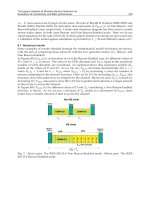
Fig. 7. The distribution of nodes in two example mesh topologies.
4.2 Random pattern of bursty traffic
In this section we investigate how the analyzes of the topologies in Fig. 3 can be applied
to more complex mesh topologies. Without loss of generality, we now focus on the two
topologies in Fig. 7 as examples, observing that the analysis can easily be generalized for
any arbitrary mesh topology. The topologies in Fig. 7 do not resemble the topologies in Fig.
3, but equations Eqs. (1)–(9) will together with Alg. (1) be able provide an upper and lower
bound for the apparent link-failure probability p
f
.
The simplest approach to analyzing a bursty traffic pattern is to generate a snapshot of the
traffic in the topology. We assume that the time between each snapshot is sufficiently long
172
Wireless Mesh Networks
The Performance of WirelessyMesh Networks with Apparent Link Failures 11
Algorithm 1

H(G, S)
Require: An undirected graph G(V, E), a directed graph S ⊆ G.
1: H
← ∅
2: for i

∈ V(G) do
3: J
←{j,∀j : 
i,j
∈ E(G)}
4: for n
∈ J do
5: R
←{r, ∀r = i : 
n,r
∈ E(G)}
6: for k
∈ R do
7: if
|{j, ∀j : 
k,j
∈ E(S)}| > 0 ∧ k /∈ G
i
then
8: h
u
← h
u
+ 1
9: end if
10: end for
11: N
← ∅
12: for k
= 0 to 2

|R|
do
13: n
i
← 0; ca ← ∅
14: for p
= 0 to |R| do
15: if k
rshift
−−−→p&1 ∧
n,R
p
∈ E(S) then
16: ca
← ca ∪
n,R
p
17: n
i
← n
i
+ 1
18: end if
19: end for
20: if not
[
∃
z:
n,z
∈ca ∧∃w=z:

n,w
∈ca:
z,w
∈E(G)
]
then
21: N
← N ∪ n
i
22: end if
23: end for
24: h
l
← 
1
|N|
∑
|N|
k= 0
N
k

25:

L ← (i, n)
26: H ←{H }∪{(

L, h
u
, h

l
,|{j, ∀j : 
n,j
∈ E(S)}|?0 : 1))}
27: end for
28: end for
29: return H
for the traffic patterns of each snapshot to be considered independent and that for each link
in the topologies in Fig. 7, a burst of data packets is transmitted with the probability p
tx
.
Each node generates data packets within a burst according to a Poisson process with the rate
parameter λ
c
. If the topology is described as a graph G(V, E), the traffic pattern given by the
graph S
(V,E, p
tx
)⊆G is a snapshot that will represent a possible data transmission pattern.
By generating a large number of random snapshots for a given p
tx

S
i∈{0,M}

, the overall
average apparent link-failure probability for a given λ
c
can be found.
Fig. 8 shows the average upper and lower bound for the apparent link-failure probability

for λ
c
=0.2. The apparent link-failure probability for the topologies in Fig. 7 is calculated
using Alg. (1) and Eqs. (1)–(9) on the randomly generated traffic patterns. The figure also
shows simulation results for the average apparent link-failure. As the simulation results
demonstrate, the analytical upper and lower bounds provide a good indicator of the average
link-failure probability even though it can be seen that the gap between the upper and lower
bound increases as p
tx
→1. This is a result of a complex traffic pattern and interaction between
the nodes that the simple model does not incorporate. At low values for p
tx
, the model’s upper
and lower bound is as expected, more accurate.
173
The Performance of Wireless Mesh Networks with Apparent Link Failures
12 Wireless Mesh Networks
(a) Results for topology in Fig. 7(a) (b) Results for topology in Fig. 7(b)
Fig. 8. Apparent link-failure probability for Fig. 7 (λ
c
= 0.2). Simulation results are shown
with a 95% confidence interval.
In Fig. 9 the upper and lower bound link-failure probability for different values of λ
c
is shown.
As can be seen from the figure, for small and large values of λ
c
, the gap between lower and
upper bound is negligible. The reason for this is that when λ
c

0, the sum of the packets
awaiting transmission in the buffers of the hidden nodes is almost zero in both the isolated
and the connected cases. Therefore, the apparent link-failure probabilities are almost identical.
For the case when λ
c
1, the sum of packets awaiting transmission in the buffers of the hidden
nodes is always greater that zero, i.e. there is always a packets waiting to be transmitted.
Hence, the difference in apparent link-failure probability is almost negligible. For 0.2
<λ
c
<0.6,
there exist various combinations of empty and non-empty buffers for the isolated and the
connected cases, thus it is expected that there will be a difference in the upper and lower
bound.
5. Network availability
If a network operates successfully at time t
0
, the network reliability yields the probability that
there were no failures in the interval
[0, t] Shooman (2002). The analysis of network reliability
assumes for simplicity that there are no link repairs in the network. This is not exactly true for
mesh networks, since a link-maintenance mechanism will ensure that a failed link is restored.
The metric used to describe repairable networks is availability. The network availability is
defined as the probability that at any instant of time t , the network is up and available, i.e. the
portion of the time the network is operational Shooman (2002). This section focuses on the
availability at the steady-state, found as t
→∞, i.e. when the transient effects from the initial
conditions are no longer affecting the network.
A typical availability measure is the k-terminal availability, namely the probability that a given
subset k of K nodes are connected. For a graph G

(V,E, p), the k-terminal availability for the k
nodes
⊆ V(G) can be found as:
174
Wireless Mesh Networks
The Performance of WirelessyMesh Networks with Apparent Link Failures 13
0.1 0.2 0.3 0.4 0.5 0.6 0.7 0.8 0.9 1.0
Probability of traffic on a link (p
tx
)
0.0
0.2
0.4
0.6
0.8
1.0
Probability of apparent link failure (p
f
)
λ =0.1
λ =0.2
λ =0.3
λ =0.4
λ =0.5
λ =0.9
Upper bound (Connected)
Lower bound (Isolated)
(a) Results for topology in Fig. 7(a)
0.1 0.2 0.3 0.4 0.5 0.6 0.7 0.8 0.9 1.0
Probability of traffic on a link (p

tx
)
0.0
0.2
0.4
0.6
0.8
1.0
Probability of apparent link failure (p
f
)
λ =0.1
λ =0.2
λ =0.3
λ =0.4
λ =0.5
λ =0.9
Upper bound
Lower bound
(b) Results for topology in Fig. 7(b)
Fig. 9. Analytical results for the upper/lower bound of the apparent link-failure probability
for the topologies in Fig. 7.
P
A
(K = k)=
|E(G)|
∑
i=w
k
(G)

T
k
i
(G)(1 − p)
i
p
|E(G)|−i
(10)
= 1 −
|E(G)|
∑
i=β(G)
C
k
i
(G)p
i
(1 − p)
|E(G)|−i
(11)
where T
k
i
(G) in Eq. (10) denotes the tieset with cardinality i, i.e. the number of subgraphs
connecting k nodes with i edges. Furthermore, w
k
(G) is the size of the minimum tieset
connecting the k nodes. In Eq. (11), C
k
i

(G) denotes the number of edge cutsets of cardinality i
and β
(G) denotes the cohesion.
5.1 k -terminal availability with apparent link-failures
The network availability (Eq. (11)) is a measure of the robustness of a wireless mesh network
and is determined by the structure and the link-failure probability of the links, provided the
node-failure probability is negligible.
For a topology described as a graph G, which includes k
−1 different distribution nodes
d
i
∈V(G) and a set of root nodes r
i
∈V(G) (normally one root node serves a set of distribution
nodes), a distribution node corresponds to a MAP while the root node corresponds to an
MPP, according to the terminology of IEEE 802.11s. For normal network operation, the transit
traffic in an IEEE802.11s network is directed along the shortest path between a root node r and
each distribution node, d
i
∈G(V). The network is not operating as expected if a distribution
node is disconnected from the root node, i.e. the network has failed. Thus, the network is
fully operational only if there is an operational path between the root node and each of the
distribution nodes. This is true if, and only if, the root node r and the k
−1 distribution nodes
175
The Performance of Wireless Mesh Networks with Apparent Link Failures
14 Wireless Mesh Networks
are all connected. Thus, the reliability of the network may be analyzed using the k-terminal
reliability.
The expression for the network availability in Eq. (11) assumes a fixed and identical

link-failure probability for all the links in a topology. However, the apparent link-failure
model can provide exact probabilities for every link in a topology. In the following
we compare the availability using an average apparent link-failure probability with the
availability using an exact and a simulated-based apparent link-failure probability.
5.1.1 k-terminal availability based on an average p
F
(P
a
A
)
As in Section 4, the average apparent link-failure probability is calculated according to Eqs.
(1)–(9) and Alg. (1). For a number of
|S|=|{S
0
, ,S
M−1
}|=5000 random patterns of bursty
traffic, the average apparent link-failure probability is expressed as:
p
F
=
1
|S|×|E(G)|
∑
s∈S
∑

i,j
∈E(G)
p

f
(i, j)
s
× p
f
(j,i)
s
(12)
where p
f
is calculated according to Eq. (9). The k-terminal availability based on an
undirectional average link-failure probability is given by:
P
a
A
[
G(V,E, p
F
)
]
= 1 −
|E(G)|
∑
i=β
C
i
(
p
F
)

i
(1 − p
F
)
|E(G)|−i
(13)
5.1.2 k-terminal availability using simulation (P
m
A
)
Using a Monte Carlo simulation, the availability of each topology is calculated where the
existence of a link 
i,j
∈E(G) depends on the probability 1 − p
F
(i, j). An estimate for the
k-terminal availability can then be calculated for s
∈S (|S|=5000) random bursty traffic patterns
as:
P
m
A
[
G(V,E, p
F
)
]
=
1
|S|

×

Number of graphs where
k nodes are connected

(14)
5.1.3 k-terminal availability using exact calculation (P
e
A
)
Since we can calculate the apparent link-failure probability of every link, it is also possible to
calculate an exact value for the k-terminal availability. Let us define L
⊆E(G) as a set of links
that are removed from the graph G
(V,E). For a traffic pattern s∈S, we define:
T
(L)
s
=
∏
∀
i,j
∈L
p
F
(i, j)
s
×
∏
∀

q,r
∈
E(G)\L
[
1−p
F
(q,r)
s
]
. (15)
An exact calculation of the k-terminal availability for
|S| bursty traffic patterns is then given
by:
P
e
A
[
G(V,E, p
F
)
]
= 1−
1
|S|
∑
s∈S
∑
∀L:V
k
(G)⊆V(G)

is not connected
T(L)
s
. (16)
5.1.4 Availability of example topologies
In this section we apply Eqs. (13)–(16) on the topologies in Fig. 7 using a scenario where the
network is configured to allow the STAs to access the MAPs at one frequency band (e.g. using
802.11b or 802.11g) and use another frequency band for the communication between the MPs.
176
Wireless Mesh Networks
The Performance of WirelessyMesh Networks with Apparent Link Failures 15
Since the extra equipment cost of such a configuration often is minimal compared with the
costs associated with site-acquisition, it is anticipated that many commercial mesh networks
will implement a MAP at each MP in the network. For such a configuration, the all-terminal
availability (P
A
(K=k)) of the network is of interest, which is shown in Fig. 10 (upper and
lower bound). The figure shows that the all-terminal availability based on an average p
F
(P
a
A
)
differs slightly from the exact calculations (P
e
A
) for the topology in Fig. 7(b). This is caused by
the fact that nodes at the border of the topology have fewer neighbors than the nodes in the
center area of the topology. For larger 2D-grid topologies, this effect will be reduced and we
will have P

a
A
≈ P
e
A
. This is easy to deduce, since the average number of neighbors in an N×N
grid network is 4
−4/N.AsN increases, the nodes in the network experience comparable
one-hop neighbor/hidden node conditions, due to the topology’s regular structure. This is
also illustrated in Fig.11(b), where the availability is calculated without the border nodes, i.e.
P
A
({c
0
, ,c
8
}).
0.0 0.2 0.4 0.6 0.8 1.0
Probability of traffic on a link (p
tx
)
0.0
0.2
0.4
0.6
0.8
1.0
Availability (P
A
(K=E) )

Lower/Upper bound (P
m
A
)
Lower/Upper bound (P
a
A
)
Lower/Upper bound (P
e
A
)
(a) Results for topology Fig.7(a) (b) Results for topology in Fig.7(b)
Fig. 10. The upper/lower bound all-terminal availability, P
A
(K=k) for the topologies in Fig.
7
(
λ
c
=0.4
)
.
6. A random geometric graph model approach to apparent link-failures
The main drawback in the previous sections is that it does not take into account correlations
between different links. For example, if two ad hoc nodes s
a
and s
b
are physically very close

to each other, and another ad hoc node s
c
is farther away, the existence of the links 
a,c
and

b,c
is expected to be correlated in reality. So far Eqs. (1)–(9) do not model this correlation.
In this section, we further extend the apparent link-failure model to encompass random
geometric graphs Haenggi et al. (2009). A random geometric graph G
(V,E,r) is a geometric
graph in which the n
= |V(G)| nodes are independently and uniformly distributed in a metric
space. In other words, it is a random graph for which a link between two nodes s
a
and s
b
exists
if, and only if, their Euclidean distance is such that
s
a
−s
b
≤r
0
, where r
0
is the transmission
range of the nodes.
177

The Performance of Wireless Mesh Networks with Apparent Link Failures
16 Wireless Mesh Networks
d
0
d
1
d
2
d
3
d
4
d
5
c
0
c
1
c
2
d
6
d
7
c
3
c
4
c
5

d
8
d
9
c
6
c
7
c
8
d
10
d
11
d
12
d
13
d
14
d
15
(a) Every node transmits with probability p
tx
= 1
and at rate λ
c
= 0.4
0.0 0.2 0.4 0.6 0.8 1.0
Probability of traffic on a link (p

tx
)
0.0
0.2
0.4
0.6
0.8
1.0
Availability (P
A
(K=E))
Upper bound (Monte Carlo)
Lower bound (Monte Carlo)
Lower bound ( ¯p
f
)
Upper bound ( ¯p
f
)
(b) Upper and lower bound all-terminal
reliability for the nodes
{c
0
, ,c
8
}.
Fig. 11. Illustration of the border effect. Since every node in {c
0
, ,c
8

} experiences equal
amount of hidden nodes, using the average apparent link-failure probability (
p
f
) gives the
same all-terminal reliability measure as the Monte Carlo simulation.
6.1 The node degree
We first establish an expression for the probability that n
0
of all n nodes are within a certain
area A
0
in the system plane Ω. The expected number of nodes per unit area is then ρ = n/Ω.
This probability is in Bettstetter (2002) shown to be:
P
(d = n
0
)=

A
0
Ω
n

n
0
n
0
!
·e

−
A
0
Ω
n
=
(
ρA
0
)
n
0
n
0
!
·e
−ρA
0
(17)
for large n and large Ω. If a node’s radio transmission range r
0
covers an area A
0
=πr
2
0
, the
probability that a randomly chosen node has n
0
neighbors is:

P
(d = n
0
)=

ρπr
2
0

n
0
n
0
!
·e
−ρπr
2
0
. (18)
A probabilistic bound for the minimum node degree of a homogenous ad hoc network is
shown to be Bettstetter (2002):
P
(d
min
≥ n
0
)=

1
−

n
0
−1
∑
i=0
(ρπr
2
0
)
i
i!
·e
−ρπr
2
0

n
. (19)
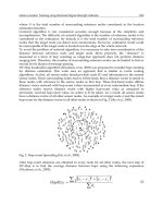
6.2 Average number of hidden nodes of an area A
0
For a given node density and transmission range, we now find the average number of hidden
nodes for any given node. Consider the intersecting circles in Fig. 12. Let us assume that the
178
Wireless Mesh Networks
The Performance of WirelessyMesh Networks with Apparent Link Failures 17
u v
r
0
r
0

d
Fig. 12. Analysis of area containing hidden nodes when node u sends a beacon to node v.
points u and v represent to nodes separated by a distance d, each with a transmission range
of r
0
. If each node covers region S
u
and S
v
when they transmit a packet, we are interested in
finding the area S
v−u
, since if any node is located in this area, this node will appear hidden
from node u. From Tseng et al. (2002) this area is given by
|S
v−u
| = |S
v
|−|S
u∩v
| = πr
2
−
INTC(d), where INTC(d) is the intersection area of the two circles:
INTC
(d)=

r
0
d/2


r
2
0
− x
2
dx. (20)
When the node v is randomly located within u’s transmission range, the average area of S
v−u
is:
S
v−u
= B
0
=
3
√
3
4π
πr
2
0
(21)
If n nodes are randomly and uniformly distributed on an area Ω following a homogenous
Poisson point process, the probability of finding b
0
nodes in the area B
0
is given by Eq. (17),
substituting A

0
with B
0
. Thus,
P
(d = b
0
)=
(
ρB
0
)
b
0
b
0
!
·e
−ρB
0
=

ρ
3
√
3
4π
πr
2
0


b
0
b
0
!
·e
−ρ
3
√
3
4π
πr
2
0
. (22)
6.3 Connectivity
A topology is said to be k-connected (k = 1, 2,3, . ) if for each node pair there exist at least k
mutually independent paths connecting them. For a topology described as a graph G
(V,E)
where |V(G)| = n, the probability that G, with n  1 where each node has a transmission
range r
0
and a homogenous node density ρ is k-connected is Bettstetter (2002):
P
(G is k-connected  P(node i has d
min
≥ k), ∀i∈V(G) . (23)
A beacon from node u to v in Fig.12 will fail to be received if any nodes in the area B
0

(S
v−u
)
transmit a data packet. The apparent link-failure probability with m hidden nodes (p
f
(m))
is given by Eq. (9). From Eq.(22), we can easily find the probability that node u in Fig. 12
has zero hidden nodes to be e
−ρB
0
. The probability that the link between node u and v is
operational if k nodes are located within node u’s transmission range can be calculated as:
p
ok
(k)=e
−ρB
0
+
n−k
∑
m=1
(
ρB
0
)
m
m!
·e
−ρB
0


1
−

p
f
(m)

2

. (24)
If we make the assumption that the one-hop links of node u fail independently, the probability
that k of the links are operational is:
P
(node u is k-connected)=P(d
min
≥ k)=
n
∑
i=k
(1 − [1 − p
ok
(k)]
i
) ·
(
ρA
0
)
i

i!
·e
−ρA
0
. (25)
179
The Performance of Wireless Mesh Networks with Apparent Link Failures
18 Wireless Mesh Networks
Fig. 13. P(k-connected) with usual Euclidian distance metric. A = 1000 ×1000 (ρ = 5 · 10
−4
)
The probability that a graph G
(V,E) where |V(G)| is k-connected is given by:
P
(G is k-connected) 

n
∑
i=k
(1−[1−p
ok
(k)]
i
) ·
(
ρA
0
)
i
i!

·e
−ρA
0

n
. (26)
Fig. 13 shows the probability of a topology with n
= 500 nodes being at least 1-connected, i.e.
P
(d
min
≥ 1). The apparent link-failure probability (p
f
) is calculated using the lower bound.
Every node in the topology transmits data packets with probability p
tx
= 1 which are Poisson
distributed with parameter λ
c
. Both analytical and Monte Carlo simulation results are shown.
The simulation results are based on 1000 randomly generated topologies from which links are
removed based on traffic load and the number of hidden nodes of a link. As the figure shows,
the simulation results match well with the analytical model. Also, the probability that the
topology is connected increases as the transmission range of the nodes is gradually increased,
which is as expected. The figure also demonstrates that more neighbors are needed in order
to have a connected topology as λ
c
, i.e. the traffic rate of the hidden nodes is increased.
7. Using unicast beacon in the presence of apparent link-failures
Having studied the probability of apparent link-failures and its effect on network availability,

it is also of interest to explore the measures for diminishing the influence of apparent
link-failures. There are several methods for this purpose, such as:
– Increasing beacon loss parameter (θ): This method will require more consecutive beacon
loss before a node determines that the link is inoperable. However, in cases where a node or
a link becomes permanently unavailable due to other reasons than apparent link-failures,
this will result in a longer time interval before a new route is calculated; and
– Reducing hysteresis (θ
h
): This method will bring a link back to operational much faster,
however it can result in oscillation between an operational and non-operational state of the
link.
Another simple yet effective solution to apparent link-failures is to introduce unicast beacon
transmissions. This method has the advantage that the MAC layer will retransmit the beacon
180
Wireless Mesh Networks
The Performance of WirelessyMesh Networks with Apparent Link Failures 19
s
0
s
1
s
2
time
Beacon
{
s
1
}
Beacon
{

s
1
}
Beacon
{
s
1
}
Data
UBReq(s
0
)
UBResp(s
1
)
(a) Explicit unicast beacon
s
0
s
1
s
2
time
Beacon
{
s
1
}
Beacon
{

s
1
}
Beacon
{
s
2
}
Beacon
{
s
2
}
Data
UBResp
Beacon
{
s
0
,s
2
}
(b) Implicit unicast beacon
Fig. 14. Handshake of UBReq and UBResp messages.
a defined number of times if an acknowledge is not received. In addition, it is possible to
protect the beacon using the RTS/CTS signalling of the MAC layer.
A request for a beacon is called a Unicast Beacon Request (UBReq) message and a response to
this is called a Unicast Beacon Response (UBResp ) message. Both these messages can be the
same packet format as normal beacon, with the difference that they use a unicast destination
address instead of a broadcast destination address. A unicast beacon can be triggered in either

end of a link. Consider the topology in Fig. 14(a). Let us assume that node s
0
has discovered
s
1
as a neighbor and vice versa. Then, at some point node s
2
transmits data such that node s
1
fails to receive the beacons from node s
0
. Node s
1
can then send a UBReq message to node
s
0
which answers with a UBResp message. This prevents node s
1
from defining the one-hop
link to node s
0
as inoperable. The UBReq and UBResp messages will also be vulnerable to
overlapping transmissions from hidden nodes. To overcome this, the link sensing mechanism
can protect the UBReq and UBResp messages using RTS/CTS at the MAC layer.
Now consider Fig. 14(b). A UBResp could also be triggered implicitly if node s
0
receives
broadcast beacons from node s
1
but fails to find its address in the beacon message. This

indicates that s
1
has not received broadcast beacons from node s
0
. Node s
0
could therefore
send a UBResp message to node s
1
, indicating that it can hear node s
1
, whereupon node s
1
will include s
0
in its next beacon.
We implemented the unicast beacon scheme in ns2 by modifying the OLSR routing protocol,
allowing unicast beacons to be protected by RTS/CTS signalling. Using No Route To Host
packets drop as an indicator, we can calculate the availability of a network. The simulation
parameters are shown in Table 2 and the topologies are shown in Fig.7.
IP/MAC layer Values Physical layer Values Simulation Values
Data 1500 Propagation Free Space Simulation/ 500s/25s
bytes model transient time
MAC CSMA/CA Data rate 11Mbps Traffic/ Poisson
protocol Distribution
Queue Length 10 Replications 50 times
Table 2. ns2 simulation parameters.
Fig.15 illustrates the all-terminal availability. The analytical and simulated results are shown
for normal OLSR beacon scheme. As can be observed from the figure, the simulated average
availability for OLSR is much lower than the analytical one. This is as expected, since our

181
The Performance of Wireless Mesh Networks with Apparent Link Failures
20 Wireless Mesh Networks
(a) Availability for the topology in Fig.7(a) (b) Availability for the topology in Fig.7(b)
Fig. 15. Average availability for the topologies in Fig.7. Results for standard beacon
transmission and unicast beacon transmission protected by RTS/CTS are shown.
(a) Throughput node d
0
→ d
5
in Fig.7(a) (b) Throughput node d
8
→ d
7
in Fig.7(b)
Fig. 16. Average throughput for the topologies in Fig.7. Results for standard beacon
transmission and unicast beacon transmission protected by RTS/CTS are shown. The source
nodes transmit at a fixed rate of 200 kbps while the load on all links is gradually increased.
182
Wireless Mesh Networks
The Performance of WirelessyMesh Networks with Apparent Link Failures 21
simple model does not take MAC retransmissions into account. MAC retransmissions will
increase the average load (λ
c
) on the channel, thus increasing the probability of beacon
loss.The figure also shows that the simulated results from unicast beacon scheme provide
much higher availability as the load on the channel increases.
8. Conclusions
This chapter introduces an approximate model for the probability of apparent link-failures in
beacon-based link maintenance schemes. The model is extended to provide a rough upper and

lower bound for arbitrary topologies. Through extensive simulations, it has been confirmed
that the model provides acceptable accuracy for simple topologies. Furthermore, more
advanced topologies with random traffic patterns and bursty traffic have been studied, where
the model can provide an average upper and lower bound for the link-failure probability with
satisfactory accuracy. In addition, the work has demonstrated how the apparent link-failure
model can be used to investigate the availability of mesh topologies and that using an
average apparent link-failure probability can serve as a good indicator for the availability
of a given topology. However, the k-terminal reliability problem is known to belong to a
class of NP-complete problems Valiant (1979), which has similar complexity as calculating the
exact network availability. Applying approximate methods to the k-terminal probability is
possible, but this is a topic for future work. In order to provide intuition about the effects of
apparent link-failures in large network with randomly distributed nodes, random geometric
graph analysis has been applied. Based on existing work on random geometric graphs, we
have extended our link-failure model so that connectivity calculations can be performed for
topologies where apparent link-failures are present.
Last but not least, a simple remedy for apparent link-failures has been introduced where
unicast beacons are used to mitigate beacon loss caused by overlapping transmissions.
This solution has been implemented for the OLSR routing protocol and the performance
improvements have been verified using the ns2 simulation tool.
9. References
Ali, H. M., Naimi, A. M., Busson, A. & V
`
eque, V. (2009). Signal strength based link sensing for
mobile ad-hoc networks, Telecommunication Systems 42(3-4): 201–212.
Bettstetter, C. (2002). On the minimum node degree and connectivity of a wireless multihop
network, MobiHoc ’02: Proceedings of the 3rd ACM international symposium on Mobile ad
hoc networking & computing, ACM, New York, NY, USA, pp. 80–91.
Chlamtac, I., Conti, M. & Liu, J. J N. (2003). Mobile ad hoc networking: Imperatives and
challenges, Ad Hoc Networks, Elsevier 1(1): 13–64.
Clausen, T. & Jacquet, P. (2003). Optimized link state routing protocol (olsr), ietf rfc 3626.

Dubey, A., Jain, A., Upadhyay, R. & Charhate, S. (2008). Performance evaluation of wireless
network in presence of hidden node: A queuing theory approach, Modeling and
Simulation, 2008. AICMS 08. Second Asia International Conference on, pp. 225–229.
Egeland, G. & Engelstad, P. E. (2009). The availability and reliability of wireless multi-hop
networks with stochastic link failures, IEEE J.Sel. A. Commun. 27(7): 1132–1146.
Egeland, G. & Engelstad, P. E. (2010). A model for the loss of Hello-Messages in a wireless
mesh network, IEEE ICC 2010 - Ad-hoc, Sensor and Mesh Networking Symposium, Cape
Town, South Africa.
Egeland, G. & Li, Y, F. (2007). Prompt route recovery via link break detection for proactive
183
The Performance of Wireless Mesh Networks with Apparent Link Failures
22 Wireless Mesh Networks
routing in wireless ad hoc networks, 10th International Symposium Wireless Personal
Multimedia Communications (WPMC), Jaipur, India.
Gerharz, M., Waal, C. D., Frank, M. & Martini, P. (2002). Link stability in mobile wireless
ad hoc networks, In Proceedings of the 27th Annual IEEE Conference on Local Computer
Networks (LCN’02).
Gharavi, H. & Kumar, S. (2003). Special issue on sensor networks and applications, Proceedings
of the IEEE 91(8).
Haenggi, M., Andrews, J., Baccelli, F., Dousse, O., Franceschetti, M. & Towsley, D. (2009).
Guest editorial: geometry and random graphs for the analysis and design of wireless
networks, Selected Areas in Communications, IEEE Journal on 27(7): 1025 –1028.
IEEE802.11 (1997). Wireless LAN medium access control (MAC) and physical layer (PHY)
specification.
IEEE802.11s (2010). Lan/man specific requirements - part 11: Wireless medium access control
(mac) and physical layer (phy) specifications: Amendment: Ess mesh networking.
Kleinrock, L. (1975). Theory, Volume 1, Queueing Systems, Wiley-Interscience.
Kleinrock, L. & Tobagi, F. (1975). Packet switching in radio channels: Part i–carrier sense
multiple-access modes and their throughput-delay characteristics, Communications,
IEEE Transactions on 23(12): 1400–1416.

Li, F., Bucciol, P., Vandoni, L., Fragoulis, N., Zanoli, S., Leschiutta, L. & L
´
azaro, O. (2010).
Broadband internet access via multi-hop wireless mesh networks: Design, protocol
and experiments, Wireless Personal Communications .
URL: />Ng, P. C. & Liew, S. C. (2004). Re-routing instability in ieee 802.11 multi-hop ad-hoc
networks, Local Computer Networks, 2004. 29th Annual IEEE International Conference
on, pp. 602–609.
ns2 (2010). The Network Simulator NS-2, />Perkins, C., Belding-Royer, E. & Das, S. (2003). Ad hoc on-demand distance vector (aodv)
routing, ietf rfc 3561.
Ray, S., Carruthers, J. B. & Starobinski, D. (2004). Evaluation of the masked node problem in
ad-hoc wireless lans, IEEE Transactions on Mobile Computing 4: 430–442.
Ray, S., Starobinski, D. & Carruthers, J. B. (2005). Performance of wireless networks with
hidden nodes: a queuing-theoretic analysis, Comput. Commun. 28(10): 1179–1192.
Shooman, M. L. (2002). Reliability of Computer Systems and Networks: Fault Tolerance, Analysis,
and Design, John Wiley and Sons, Inc.
Tobagi, F. & Kleinrock, L. (1975). Packet switching in radio channels: Part ii–the hidden
terminal problem in carrier sense multiple-access and the busy-tone solution,
Communications, IEEE Transactions on 23(12): 1417–1433.
Tseng, Y C., Ni, S Y., Chen, Y S. & Sheu, J P. (2002). The broadcast storm problem in a mobile
ad hoc network, Wirel. Netw. 8(2/3): 153–167.
Valiant, L. G. (1979). The complexity of computing the permanent, Theor. Comput. Sci.
8: 189–201.
Voorhaen, M. & Blondia, C. (2006). Analyzing the impact of neighbor sensing on the
performance of the olsr protocol, Modeling and Optimization in Mobile, Ad Hoc and
Wireless Networks, 2006 4th International Symposium on, pp. 1–6.
184
Wireless Mesh Networks
0
Pursuing Credibility in Performance Evaluation of

VoIP Over Wireless Mesh Networks
Edjair Mota
1
, Edjard Mota
1
, Leandro Carvalho
1
,
Andre Nascimento
1
and Christian Hoene
2
1
Federal University of Amazonas
2
T¨ubingen University
1
Brazil
2
Germany
1. Introduction
There has been an increasingly interest in real-time multimedia services over wireless
networks in the last few years, for the most part due to the proliferation of powerful mobile
devices, and the potential ubiquity of wireless networks. Nevertheless, there are some
constraints that make their deployment over Wireless Mesh Networks (WMNs) somewhat
difficult. Due to the dynamics of WMNs, there are significant challenges in the design
and optimization of such services. Impairments like packet loss, delay and jitter affects the
end-to-end speech quality (Carvalho, 2004). Experimenters have been proposing solutions to
the challenges found so far, and comparing them before implementation is a mandatory task.
There exists a necessity of designing efficient tools for enhancing the computational effort of

the performance modeling and analysis of VoIP over WMNs. Structural complexity of such
highly dynamic systems causes that in many situations computer simulation is the only way
of investigating their behavior in a controllable manner, allowing the experimenter to conduct
independent and repeatable experiments, in addition to the comparison of a large number
of system alternatives. Stochastic simulation is a flexible, yet powerful tool for scientifically
getting insight into the characteristics of a system being investigated. However, to ensure
reproducible results, stochastic simulation imposes its own set of rules. The credibility
of a performance evaluation study is greatly affected by the problem formulation, model
validation, experimental design, and proper analysis of simulation outcomes.
Therefore, a fine-tuning of the parameters within a simulator is indispensable, so that it closely
tracks the behavior of a real network. However, the lack of rigor in following the simulation
methodology threatens the credibility of the published research (Pawlikowski et al., 2002;
Andel & Yasinac, 2006; Kurkowski et al., 2005).
The aim of this chapter is to provide a detailed discussion of these aspects. To do so, we
used as a starting point the observation that the optimized use of the bandwidth of wireless
networks definitely affects the quality of VoIP calls over WMN. Since the payload size of
VoIP packets is usually smaller than the header size, much network resource is spent for
conveying control information instead of data information. Hence, VoIP header compression
is an alternative to reduce the use of the bandwidth needed to transmit control information,
thereby increasing the percentage of bandwidth used to carry payload information.
9
Andréa
2 Wireless Mesh networks
However, this mechanism can make the VoIP system less tolerant to packet loss, which
can be harmful in WMN, due to its high rate of packet loss. Additionally, in a multi-hop
wireless environment, simple schemes of header compression may not be enough to increase
or maintain the speech quality. An interesting alternative approach in this context is the use
of header compression in conjunction with packet aggregation (Nascimento, 2009), aiming to
eliminate the intolerance to packet loss without reducing the compression gain.
Although these issues are not unique to simulation of multimedia transmission over wireless

mesh networks, we focus on issues affecting the WMN research community interested in VoIP
transmissions over WMN. After modeling thoroughly the issues of VoIP over WMN, we built
a simulation model of a real scenario at the Federal University of Amazonas, where we have
been measuring the speech quality of VoIP transmissions by means of a tool developed by
our groups. Then, we modeled a bidirectional VoIP traffic, and proposed a carefully selected
set of experiments and simulation details such as the sources of randomness and analysis of
the output data, closely following sound methodology for each phase of the experimentation
with simulation.
2. Background
2.1 Wireless mesh networks
Wireless mesh network (WMN) is a promising communication technology that has been
successfully tested in academic trials and is a mature candidate to implement metropolitan
area networks. Compared to fiber and copper based access networks, it can be easily
deployed, maintained and expanded on demand. It offers network robustness, and reliable
service coverage, besides its low costs of installation and operation. In many cities, such as
Berlin and Bern, WMN has been used to provide Internet access for many users.
In its more general form, a WMN consists of a set of wireless mesh routers (WMRs) that
interconnect with each other via wireless medium to form a wireless backbone. These WMRs
are usually stationary and work as access points or gateways to the Internet to wireless mesh
clients (WMCs). High fault tolerance can be achieved in the presence of network failures,
improper operation of WMRs, or wireless link inherent variabilities. Based on graph theory,
(Lili et al., 2009) suggested a method to analyze the fault-tolerant and communication delay
in a wireless mesh network, while (Queiroz, 2009) investigated the routing table maintenance
issue, by proposing and evaluating the feasibility of applying the Bounded Incremental
Computation model (Ramalingam & Reps, 1996) to satisfy scalability issues. Such kind of
improvement is essential to real time multimedia application in order to reduce the end-to-end
delay.
Even being accepted as a good solution to provide access to the telephone service, the WMN
technology poses some problems being currently investigated such as routing algorithms,
self-management strategies, interference, to say a few. To understand how to achieve the

same level of quality of multimedia applications in wired networks, it is imperative to grasp
the nature of real-time multimedia traffic, and then to compare it against the problems related
to the quality of multimedia applications.
2.2 Voice over IP
A VoIP call placed between two participants requires three basic types of protocol: signaling,
media transmission, and media control. The signaling protocols (e.g. H.323, SIP) establish,
maintain and terminate a connection, which should be understood as an association between
applications, with no physical channel or network resources associated with it. The media
186
Wireless Mesh Networks
Pursuing Credibility in Performance Evaluation of VoIP Over Wireless Mesh Networks 3
transmission protocols (e.g. RTP) are responsible for carrying out the actual content of the
call – the speaker’s voice – encoded in bits. Finally, the media control protocols (e.g. RTCP)
convey voice packet transmission parameters and statistics, ensuring better end-to-end packet
delivery. In this work, our attention is focused upon the voice stream. So, lets briefly introduce
the main logical VoIP components of the media transmission path.
As illustrated in Figure 1, the sender’s voice is captured by a microphone and digitalized by an
A/D conversor. The resulting discrete signal is then encoded and compressed by some codec
into voice frames. One or more frames can be encapsulated into a voice packet by adding RTP,
UDP and IP headers. Next, the voice packets are dispatched to the IP network, where they
can get lost due to congestion or transmission errors. The transmission delay of packets – i.e,
the time needed to deliver a packet from the sender to the receiver – is variable and depends
on the current network condition and the routing path (Hoene et al., 2006).
At the receiver, the arriving packets are inserted into a dejitter buffer, also known as playout
buffer, where they are temporarily stored to be isochronously played out. If packets are too
late to be played out in time, they are discarded and considered as lost by the application.
After the dejitter buffer the speech frames are decoded. If a frame is missing, the decoder
fills the gap by applying some Packet Loss Concealment (PLC) algorithm. Finally, the digital
signal is transformed into an acoustic signal.
Since IP networks were not designed to transport real-time traffic, an important aspect in

VoIP communications is the assessment of speech quality. It is imperative that new voice
services undergo a significant amount of testing to evaluate their performance. Speech
quality is a complex psychoacoustic outcome of the perception process of the human auditory
system (Grancharov & Kleijn, 2008). Its measurement can be carried out using either
subjective or objective methods.
Subjective methods, specified in ITU-T Rec. P.800 (ITU-T, 1996), require that a pool of listeners
rates a series of audio files using a five-level scale (1 – bad, 2 – poor, 3 – fair, 4 – good, 5 –
excellent). The average of all scores thus obtained for speech produced by a particular system
represents its Mean Opinion Score (MOS). The main reason for the popularity of this test is its
simplicity (Grancharov & Kleijn, 2008). However, the involvement of human listeners makes
them expensive and time consuming. Moreover, subjective tests are not suitable to monitor
the QoS of a network on a daily basis. This has made objective methods very attractive for
meeting the demands for voice quality measurement in communications networks.
Among the objective (or instrumental) methods, the E-model, defined in the ITU-T Rec. G.107
(ITU-T, 1998), is one of the most used. It computes, in a psychoacoustic scale, the contribution
of all impairment factors that affect voice quality. This does not imply that the factors are
uncorrelated, but only that their contributions to the estimated impairments are independent
and each impairment factor can be computed separately (Myakotnykh & Thompson, 2009).
Although initially designed for transmission planning of telecommunication systems (Raake,
2006; ITU-T, 1998), the E-model was modified by (Clark, 2003; Carvalho et al., 2005) to be used
for VoIP network monitoring.
The output of the E-model is the R factor, which ranges from 0 (worst) to 100 (excellent) and
;
ͬ ŶĐŽĚĞƌ
ZdWͬ
hWͬ/W
ͬ
ĞũŝƚƚĞƌ
ďƵĨĨĞƌ
ZdWͬ

hWͬ/W
ĞĐŽĚĞƌ
/W
EĞƚǁŽƌŬ
^ĞŶĚĞƌ ZĞĐĞŝǀĞƌ
Fig. 1. VoIP components of the media transmission path.
187
Pursuing Credibility in Performance Evaluation of VoIP Over Wireless Mesh Networks
4 Wireless Mesh networks
can be converted to the MOS scale. Voice calls whose R factor value is below 60 (or 3.6 in MOS
scale) are not recommended (ITU-T, 1998). For VoIP systems, the R factor can be obtained by
the following simplified expression (Carvalho et al., 2005):
R
= 93.2 − Id(codec, del ay) − Ie,ef f(codec, loss,PLB) (1)
where Id represents the impairments associated with end-to-end delay, and Ie,ef f represents
the impairments associated with codec compression, packet loss rate and packet loss behavior
(PLB) during the call.
The measurement tool proposed in (Carvalho et al., 2005) for speech quality evaluation based
on the E-model was adapted as a patch to the Network Simulator code (McCanne & Floyd,
2000). It was used for validating our simulation models concerning the transmission of VoIP
over WMNs.
2.3 Performance evaluation
Measurement and stochastic simulation are the main tools commonly used to assess the
performance of multimedia transmission over WMNs. Success in the development of complex
wireless networks is partially related to the ability of predicting their performance already in
the design phase and subsequent phases of the project as well. Dynamic increasing of the
complexity of such networks and the growth of the number of users require efficient tools
for analyzing and improving their performance. Analytical methods of analysis are neither
general nor detailed enough, and in order to get tractability, they need sometimes to make
assumptions that require experimental validation. On the other hand, simulation, formerly

known as a last resort method, is a flexible and powerful tool adequate for prototyping such
complex systems. To the factors that have additionally stimulated the use of simulation,
one could include: faster processors, larger-memory machines and trends in hardware
developments (e.g. massively parallel processors, and clusters of distributed workstations).
Straightforward simulation of complex systems, such as WMNs, takes frequently a
prohibitively amount of computer time to obtain statistically valid estimates, despite
increasing processing speed of modern computers. It is not rare the simulation take some
hours to estimate a performance metric corresponding to a few seconds of real time. (Mota
et al., 2000) investigated the influence of jitter on the quality of service offered by a wireless
link, and reported a simulation time as long as 180 hours using just 9 wireless terminals,
though simulation has been executed in a fast workstation dedicated to that purpose.
Such phenomenon results from the statistical nature of the simulation experiments. Most
simulation models contain stochastic input variables, and, thereby, stochastic output
variables, the last ones being used for estimating the characteristics of the performance
parameters of the simulated system. In order to obtain an accurate estimate with known
(small) statistical error, it is necessary to collect and analyze sequentially a substantial amount
of simulation output data, and this can require a long simulation run.
Efficient statistical tools can be used to impact the running time of an algorithm by choosing an
estimator with substantially lower computational demand. It would be a mistake to think that
more processing power can replace the necessity for such tools, since the associated pitfalls can
be magnified as well (Glynn & Heidelberger, 1992). The need for effective statistical methods
to analyze output data from discrete event simulation has concerned simulation users as early
as (Conway, 1963). Development of accurate methods of statistical analysis of simulation
output data has attracted a considerable scientific interest and effort.
188
Wireless Mesh Networks