Access-Point Allocation Algorithms for Scalable
Wireless Internet-Access Mesh Networks
11
method algorithm manual
#ofAPs 10 17
max. hop count 1 2
1-NIC throughput (Mbps) 30.96 22.79
2-NIC throughput (Mbps) 47.74 46.26
Table 3. AP allocation results for network field 2
However, for the 2-NIC case, the advantage becomes small by allowing the enough bandwidth
for communications between APs.
2.5.5 Network field 3
Finally, we examine the third network field as the more practical and harder one similar to a
building floor in our campus. This field is composed of two rows of different-sized rectangular
rooms and one corridor. One row has 12 small square rooms with 5m
× 5m size with 4 host
points, and another row has 5 large rectangular rooms with 10m
× 12.5m size with 20 host
points. The host points along the walls parallel to the corridor are selected as battery points.
Besides, 29 battery points are allocated with the same interval in the corridor with no host
association. The battery point in front of the center of the fifth small room in the corridor is
selected as the GW, so that in the manual allocation, each AP in the corridor can cover three
small rooms regularly. The total number of expected hosts is 148
(= 4 ×12 + 20 × 5). The
maximum load limit L is again set 25. Thus, the lower bound on the number of APs to satisfy
the load constraint is 6
(=

148
25


).
Figure 4 shows our AP allocation using 6 APs for this field. Every AP other than the GW
has one hop distance from the GW. Thus, our algorithm found the lower bound solution. For
comparisons, a manual allocation using 9 APs is also depicted, where one AP is allocated to
each large room and 4 APs are allocated in the corridor regularly. The maximum hop count of
this manual allocation is two as shown by lines. Table 4 compares the throughputs between
two allocations, where our allocation provides the better throughput than the manual one for
both 1-NIC and 2-NIC cases.
2.5.6 Effect of estimation error of log-distance path loss model
The estimation error of the log-distance path loss model in (1) may have the considerable
impact to the result of our algorithm. To estimate this impact briefly, we calculate the
percentage of the received signal strength drop in the real world from the estimation that
Fig. 4. AP allocations for network field 3.
39
Access-Point Allocation Algorithms for Scalable Wireless Internet-Access Mesh Networks
12 Wireless Mesh Networks
method algorithm manual
#ofAPs 6 9
max. hop count 1 2
1-NIC throughput (Mbps) 33.19 27.16
2-NIC throughput (Mbps) 55.54 52.58
Table 4. AP allocation results for network field 3
causes the disconnection at the AP allocation. As shown in Table 5, this percentage is
distributed from 3% in the network field 1 to 30% in the field 3. In our future works, we will
improve our algorithm in terms of the robustness to the estimation error of the log-distance
path loss model, such that the connectivity is maintained while the interference is curbed even
if the model has the error.
2.6 Related works
Several papers have reported studies of AP placement algorithms for conventional WLANs.
Within our knowledge, the same AP allocation problem in the wireless mesh network for

the Internet access in indoor environments has not been reported before. In fact, most of the
papers focus on the construction of WLAN without considering wireless connections between
APs, or on the GW placement for the wireless mesh networks.
In (Lee et al., 2002), Lee et al. study simple ILP formulations for the AP placement and channel
assignment problems in conventional WLANs, using discrete placement formulations. Their
algorithm finds best AP associations of host points to minimize the maximum channel
utilization among APs. In their WLANs, APs are connected with each other through wired
connections, whereas our AP allocation problem must satisfy the connectivity among APs
through wireless connections. This additional constraint makes the problem much harder,
because it usually requires the more number of APs to provide wireless connections between
them while the number of APs should be minimized to reduce the cost and the interference
between links. Besides, their algorithm does not consider the minimization of APs and their
transmission powers.
In (Kouhbor, Ugon, Rubinov, Kruger & Mammadov, 2006), Kouhbor et al. investigate
the AP allocation problem in indoors for WLANs with a path loss model to calculate the
coverage area of an AP. They present a continuous mathematical model of finding AP
locations to cover every user while avoiding insecure locations, which is solved by their
global optimization algorithm. The effectiveness is verified through simulating one real
building floor. They observe that the dimension of the building, the number of users and their
locations, the transmission power, and its received threshold have effects on the AP allocation.
Unfortunately, they do no consider the wireless connection constraint, like (Lee et al., 2002).
In (Bahri & Chamberland, 2005), Bahri et al. study the problem of designing a conventional
WLAN, and propose an optimization model for selecting the location, the power, and the
channel for each AP. They propose a Tabu search heuristic algorithm to improve this solution.
network field 1 network network
corner side center field 2 field 3
3% 3% 4% 12% 30%
Table 5. Percentage of received signal strength drops for AP allocation failure
40
Wireless Mesh Networks

Access-Point Allocation Algorithms for Scalable
Wireless Internet-Access Mesh Networks
13
The results are compared to lower bounds obtained by relaxing a subset of the constraints
in their model, and show that this heuristic produces relatively good solutions rapidly. It is
significant to develop the lower bound formulation in order to precisely evaluate the proposed
heuristic, and to explore exact algorithms to solve small-size instances of the problem.
In (Chandra et al., 2004), Chandra et al. formulate the Internet transit access point
placement problem under various wireless models. This problem aims to provide the Internet
connectivity in multihop wireless networks. If we consider the Internet transit access point as
a GW, their network model is the same as WIMNET where every AP becomes a GW.
In (Wu & Hsieh, 2007), Wu et al. investigate the impact of multiple wireless mesh networks
that are overlapped in a service area. They formulate the resource sharing problem as an
optimization problem, and present a general LP formulation. They consider the optimization
of the number and the selection of bridge nodes. Simulation results show that if a proper
interworking is provided between overlapped networks, significant performance gain can be
obtained.
In (Li et al., 2007), Li et al. study the GW placement problem for the throughput optimization
in wireless mesh networks, given the traffic demand for each node, the number of GWs,
and the interference model. They present an LP formulation to find a periodic TDMA link
scheduling to maximize the throughput for given GW locations. Then, by applying it with
every possible combination of the grid points superimposed on the field for GW locations,
they find the best GW layout.
In (Robinson et al., 2008), Robinson et al. study the GW placement problem for the
wireless mesh network. They present a technique to efficiently compute the GW-limited
fair capacity as a function of the contention at each GW, and two GW placement algorithms.
The first MinHopCount adapts a local search algorithm for the capacitated facility location
problem in (Pal et al., 2001) that is composed of add, open, and close operations. The second
MinContention adopts a swap-based local search algorithm for the incapacitated k-median
problem with a provable performance guarantee.

In (Naidoo & Sewsunker, 2007), Naidoo et al. discuss the use of Mesh technology as a strategy
to extend coverage to provide rural telecommunication services. Their study investigates
the range extension using a hybrid wireless local area network architecture running both
infrastructure and client wireless mesh networks.
2.7 Conclusion
This section presented the two-stage AP allocation algorithm for WIMNET in indoor
environments. The effectiveness was verified through simulations using the WIMNET
simulator, where the significant performance improvement over manual allocation was
observed. The future works may include the more precise consideration of indoor
environments in the signal propagation model (Beuran et al., 2008), the algorithm
improvement in terms of the robustness to the estimation error of the model, the adoption of
the ILP formulation (Lee et al., 2002) and the global optimization algorithm (Kouhbor, Ugon,
Rubinov, Kruger & Mammadov, 2006) to the AP allocation problem, and the application to
the design of real wireless mesh networks.
3. Dependability extensions of AP allocation algorithm
3.1 Fault dependability in WIMNET
WIMNET may be disconnected by occurrence of even one link fault or one AP fault
in the AP allocation found by the algorithm in the previous section. To improve the
41
Access-Point Allocation Algorithms for Scalable Wireless Internet-Access Mesh Networks
14 Wireless Mesh Networks
dependability of WIMNET, the AP allocation algorithm should be extended to find an AP
allocation such that the APs can be connected even for one link fault or one AP fault
occurrence. This dependability can be achieved by allocating redundant APs to provide
backup routes (Ramamurthy et al., 2001). At the same time, the number of such APs and
the maximum hop count should be minimized for the cost reduction and the performance
improvement. Here, we summarize the design goal in dependability extensions of the AP
allocation algorithm as follows:
1. to endure one link fault or one AP fault,
2. to minimize the number of additional APs, and

3. to minimize the maximum hop count.
3.2 Link-fault dependability extension
3.2.1 Constraint for link-fault dependability
First, we discuss the link-fault dependability extension of the AP allocation algorithm. To
achieve the link-fault dependability, the network must be connected if any link is removed
from there. Then, another constraint must be satisfied in the AP allocation in addition to the
original six constraints in 2.2.2:
7) to provide the connectivity among the APs if any link is removed.
3.2.2 Algorithm extension for link-fault dependability
Then, we present the algorithm extension for the link-fault dependability. The idea here
is that after maximizing the transmission power from any AP to increase the connectivity,
we find any link whose removal disconnects the network, which is called the bridge. While
bridges exist, we sequentially allocate an additional AP at the battery point that can resolve the
maximum number of bridges until all of them are resolved. Then, we find the minimum-delay
routing tree to this link-fault dependable AP allocation by applying the algorithm in (Funabiki
et al., 2008). Finally, we minimize the transmission powers of APs such that the constraints
of the problem are satisfied. The following procedure describes the link-fault dependability
extension:
1. Input the AP allocation from the algorithm in (Farag et al., 2009).
2. Maximize the transmission power for any AP and find the links between two APs.
3. Find the set of bridges BR.
4. Apply the following procedure if BR
= ∅:
a. Apply the AP association refinement in 2.4.3.
b. Apply the routing tree algorithm in (Funabiki et al., 2008).
c. Minimize the transmission power of the APs such that all the constraints are satisfied.
d. Terminate the procedure.
5. For every bridge in BR, find the set of battery points that can resolve this bridge if a new
AP is allocated there. Let this set of the battery points found here be BS.
6. Calculate the number of bridges in BR for each battery point in BS that the AP allocated

there can resolve.
42
Wireless Mesh Networks
Access-Point Allocation Algorithms for Scalable
Wireless Internet-Access Mesh Networks
15
7. Find the battery point in BS that can resolve the largest number of bridges in BR, and
allocate an AP there.
8. Update BR.
9. Go to 4.
3.3 AP-fault dependability extension
3.3.1 Constraint for AP-fault dependability
Next, we discuss the AP-fault dependability extension of the AP allocation algorithm. To achieve
the AP-fault dependability, the network must be connected, and every host must be covered
by a remaining AP, if any AP is removed from there. Here, no GW is removed, assuming
no fault at GW. Then, the following two constraints must be satisfied in the AP allocation in
addition to the original six constraints in 2.2.2:
7) to cover any host by an existing AP if any AP is removed, and
8) to provide the connectivity among the APs if any AP is removed.
3.3.2 Algorithm extension for AP-fault dependability
We present the algorithm extension to the AP-fault dependability. For the AP-fault
dependability, at least the link-fault dependability must be satisfied, because if one AP is
removed from the network, its incident links are also removed. Thus, in this extension, we
use the link-fault dependable AP allocation and maximize the transmission power of any AP
as the initial state.
First, we find any host point that cannot be covered if one AP is removed from the network
due to the fault, called the critical point, in the initial state. The critical point satisfies the
following either condition:
1) only this fault AP covers it, or
2) all the backup APs reach association load limits, including the re-associated hosts by

this AP fault.
While critical points exist, we sequentially allocate an additional AP to the battery point that
can cover the maximum number of critical points until all of them are resolved. Then, we
find any AP whose removal disconnects the network, called the cut AP. While cut APs exist,
we sequentially allocate an additional AP to the battery point that can cover the maximum
number of cut APs until all of them are resolved.
After these procedures, we apply the improvement stage in 3.3.3 for finding the better AP
allocation. Then, we apply the algorithm in (Funabiki et al., 2008) to find the routing tree to
the AP-fault dependable allocation. Finally, we minimize the transmission powers such that
the constraints are satisfied. The following procedure describes the AP-fault dependability
extension:
1. Input the link-fault dependable AP allocation.
2. Maximize the transmission power for any AP and find the links between APs.
3. Find the set of critical host points CR.
4. Apply the following critical host resolution procedure until CR
= ∅:
a. For every host point in CR, find the set of battery points that can cover this critical point
if a new AP is allocated there. Let this set of the battery points found here be CS.
43
Access-Point Allocation Algorithms for Scalable Wireless Internet-Access Mesh Networks
16 Wireless Mesh Networks
b. Calculate the number of critical points in CR for each battery point in CS that the AP
allocated there can cover.
c. Find the battery point in CS that can cover the largest number of critical points in CR,
and allocate an AP there.
d. Update CR.
5. Find the set of cut APs CA.
6. Apply the following cut AP resolution procedure until CA
= ∅:
a. For every cut AP in CA, find the set of battery points that can cover this cut AP if a new

AP is allocated there. Let this set of the battery points found here be CB.
b. Calculate the number of cut APs in CA for each battery point in CB that the AP allocated
there can cover.
c. Find the battery point in CB that can cover the largest number of cut APs in CA, and
allocate an AP there.
d. Update CA.
7. Apply the improvement stage in 3.3.3.
8. Apply the AP association refinement in 2.4.3.
9. Apply the routing tree algorithm in (Funabiki et al., 2008).
10. Minimize the transmission power of the APs such that all the constraints are satisfied.
11. Terminate the procedure.
3.3.3 Improvement stage
The improvement stage for the AP-fault dependable extension has been slightly modified
from the corresponding one in the original AP allocation algorithm, such that any AP must
be connected with at least two APs in order to preserve the link/AP fault dependability. The
following procedure is repeated for a given constant number of iterations AT, where the best
solution in terms of the cost function F is always kept for the final solution during the iterative
search process:
1. Randomly select a battery point b
j
/∈ S that is connected to at least two APs in S, and add it
into S with the maximum transmission power.
2. Apply the AP association refinement in 2.4.3.
3. Remove from S any AP that satisfies the following four conditions:
1) it is different from b
j
and GW,
2) all the host points associated with the AP can be re-associated with the remaining
APs, where for the new association of each host point, the load limit constraint
is checked from the AP whose signal power is largest if two or more APs can be

associated,
3) no cut AP appears if removed, and
4) no critical host point appears if removed.
4. If removed, re-associate all the host points associated with this AP to the APs found in 2).
5. Change the transmission power of any possible AP to the smallest one in TP such that this
AP can still cover any associated host and maintain the links necessary to connect all the
APs.
44
Wireless Mesh Networks
Access-Point Allocation Algorithms for Scalable
Wireless Internet-Access Mesh Networks
17
3.4 Simulation results for dependability extensions
3.4.1 Simulated instances
In this subsection, we show simulation results for the dependability extension using the
WIMNET simulator. A network field composed of 16 square rooms with 400 host points,
and a field similar to the first floor in the central library at Cairo university as a practical
one, are considered for simulated instances. Like the previous instance, each host point is
associated with one host, and the maximum load limit L is set 25. In the latter field, the total
size is 64m
× 32m, and 411 host points are allocated, where the host points along the walls
are selected as battery points. Note that the size of the largest room at the top right, called
Taha Hussin Hall,is18m
×12m with 74 host points. The lower bound on the number of APs to
satisfy the load constraint is 17
(=

411
25


).
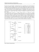
Figures 5 and 6 illustrate the network field and the AP allocation result with the routing tree
for each instance, respectively. The white circle represents an AP allocated by the original
algorithm, the gray circle does an additional AP by the link-fault dependability extension,
and the black circle does an additional AP by the AP-fault dependability extension.
3.4.2 AP allocation results
First, we discuss the solution quality in terms of the number of APs in AP allocation results
for dependability extensions. Table 6 compares the numbers of APs in the original AP
allocation algorithm, the link-fault extension, and the AP-fault extension. For the artificial
network field of 16 square rooms (Square field), our dependability extensions can provide
the link-fault dependability with additional three APs, and the AP-fault dependability with
additional ten APs. The latter result is much better than the trivial solution for the AP-fault
dependability using 15 additional APs where two APs are allocated in each room. For the
practical field in the central library (Library field), no additional AP is necessary for the
link-fault dependability and only three additional APs for the AP-fault dependability. Because
most APs can communicate with GW in one hop, any link can easily be backed up by other
Fig. 5. AP allocation result for dependability extensions in 16 square-room field.
45
Access-Point Allocation Algorithms for Scalable Wireless Internet-Access Mesh Networks
18 Wireless Mesh Networks
Fig. 6. AP allocation result for dependability extensions in central library field.
links. These results verify the effectiveness of our proposal for dependability extensions in
WIMNET in terms of the AP allocation cost.
3.4.3 Throughput results
Then, we investigate throughput changes with or without link/AP faults among AP
allocation results for dependability extensions. Table 7 compares total throughputs among AP
allocations for the three cases when no link/AP has fault. The result indicates that the total
throughput is slightly degraded as the number of APs increases for the fault dependability
extensions due to the increase of the interference among wireless links between APs using the
single channel.

Tables 8 and 9 show the average, maximum, and minimum throughputs in the link-fault
dependable and AP-fault dependable allocations when one link or AP is removed from the
network to assume the occurrence of a fault. By comparing these results, we conclude that
our proposal can provide sufficient throughputs, even if one link fault or one AP fault occurs
in WIMNET.
Here, we note that in the fault dependable AP allocation, some APs may become redundant.
Thus, the routing without using such APs may be able to improve the performance by
reducing the interference. Besides, if multiple NICs are used at APs for multiple channel
communications, the results can be changed by reducing the interference. The performance
evaluation in such cases will be in our future studies.
Instance Original Link-fault AP-fault
Square field 16 19 26
Library field 17 17 20
Table 6. Numbers of allocated APs.
46
Wireless Mesh Networks
Access-Point Allocation Algorithms for Scalable
Wireless Internet-Access Mesh Networks
19
Instance Original Link AP
Square field 13.0 12.9 12.6
Library field 23.9 23.9 23
Table 7. Total throughputs with no fault (Mbps).
Instance Ave. Max. Min.
Square field 12.4 12.9 10.9
Library field 23.37 23.74 23
Table 8. Total throughputs for link-fault extension with one link fault (Mbps).
3.5 Related works
Several studies have been reported for the dependability in multihop wireless networks
including wireless mesh networks. This subsection briefly introduces some of them.

In (Gupta & Younis, 2003), Gupta et al. presented efficient detection and recovery mechanisms
of one failed GW or its link in a clustered wireless sensor network. The detection is based on
the consensus of healthy GWs. The recovery reassociates the sensors that are managed by
the failed GW to other clusters based on the range information. The effectiveness is verified
through simulations.
In (Varshney & Malloy, 2006), Varshney et al. presented the multilevel fault tolerance design
of wireless networks using adaptable building blocks (ABBs). The ABB has several levels
of components such as base stations, base station controllers, databases, and links, similar
to cellular networks, where the reliability such as MTBF/MTTR can differ significantly
by using different number of components. The fault tolerance design is achieved at the
three levels of the component and link, the building block, and the interconnection. If the
computed dependability attributes are not acceptable, the process of adding the incremental
redundancy at the three levels is repeated. They present an analytical model of measuring
the dependability enhancement, and evaluate the network survivability and the network
availability with different interconnection architectures, block-level redundancy, mobility, and
fault tolerance at the three levels in ring, star, and SONET dual ring topologies.
In (Pan & Keshav, 2006), Pan et al. studied detection and repair methods of faulty APs
for large-scale wireless networks. For the detection, they presented three algorithms. The
first one is that if an AP gives reports to the network operation center, it is regarded as no
fault. The second one modifies the first one such that the no-fault probability of an AP is
exponentially decreased as the time interval of no report increases. The third one further
improves it by considering the path of APs that the host is moving along, where if an AP
along the path does not report, it can be regarded as a fault. For the repair, they presented the
ellipse heuristic algorithm to find the best schedule of repairing faulty APs by minimizing the
total moving length and the downtime of popular APs. They evaluate their proposal using
the free data set available from Dartmouth College that includes log messages from client
association, authentication, and others in their wireless networks for nearly four years.
Instance Ave. Max. Min.
Square field 12.31 12.6 11.1
Library field 21.75 22.65 21

Table 9. Total throughputs for AP-fault extension with one AP fault (Mbps).
47
Access-Point Allocation Algorithms for Scalable Wireless Internet-Access Mesh Networks
20 Wireless Mesh Networks
3.6 Conclusion
This section presented extensions of the AP allocation algorithm to find the link/AP-fault
dependable AP allocations, to assure the connectivity and the host coverage in case of
one link/AP fault by allocating redundant APs. The effectiveness was verified through
simulations in regular and practical network fields using the WIMNET simulator. The future
works may include the routing without using redundant APs, the evaluation of multiple
channel communications, and the reduction of APs by considering backup APs in different
GW clusters.
4. Access point clustering algorithm
4.1 AP clustering in WIMNET
As the number of APs increases in WIMNET with a single GW, the communication delay
may inhibitory increase, because the links between APs around the GW become too crowded.
Then, the adoption of multiple GWs is a reasonable solution to this problem, where the
proper clustering of the APs into a set of disjoint GW clusters is important to maximize the
performance of WIMNET.
The proper AP clustering is actually a hard task because it must consider several constraints
and optimization indices simultaneously. The first constraint is that the number of APs in a
cluster must not exceed the upper limit due to the WDS size constraint. The second one is that
all APs in a cluster must be connected with each other. The third one is that one AP in a cluster
must be selected as the GW that can deploy wired connections to the Internet. The fourth one
is that the number of hosts associated with APs in a cluster must not exceed the limit, so that
any cluster can ensure the communication bandwidth of hosts. As the optimizing indices,
the number of GW clusters should be minimized to save installation and operation costs of
the network. The communication delay between any AP and a GW in any cluster should be
minimized to enhance the performance. As a result, the APs, the GW, and the communication
routes between APs and the GW in every GW cluster must be found simultaneously.

4.2 AP clustering problem
4.2.1 Assumptions in AP clustering problem
In the AP clustering problem, we assume that the locations of the APs with battery supplies
and the wireless links between APs in the network field have been given manually, or by
using their corresponding algorithms during the design phase of WIMNET, as the inputs. The
topology of the AP network is described by a graph G
=(V, E), where a vertex in V represents
an AP and an edge in E represents a link. Each vertex is assigned the maximum number of
hosts associated with the AP as the load, and each edge is assigned the transmission speed
for the delay estimation, which are given as design parameters. A subset of V are designated
as GW candidates, where wired connections are available for the Internet access. The number
of GW clusters K greatly affects the installation and operation costs of WIMNET because the
costly Internet GW is necessary in each cluster. Thus, the number of clusters K is given in the
input, so that the network designer can decide it. Furthermore, the limit on the cluster size
and the required bandwidth in one cluster are given to determine their constraints.
4.2.2 Formulation of AP clustering problem
Now, we formulate the AP clustering problem for WIMNET as a combinatorial optimization
problem.
48
Wireless Mesh Networks
Access-Point Allocation Algorithms for Scalable
Wireless Internet-Access Mesh Networks
21
– Input: G =(V, E): a network topology with N APs (N = |V|), h
i
: the maximum number
of hosts associated with the AP
i
(the i-th AP) for i = 1,···, N, s
ij

: the transmission speed of
the ij-th link (link
ij
)fromAP
i
to AP
j
in E, X (⊆ V): a set of GW candidates, K: the number
of GW clusters, H: the limit on the number of associated hosts in a GW cluster (bandwidth
limit), and P: the limit on the number of APs in a GW cluster (cluster size limit).
– Output: C
= {C
1
,C
2
,···, C
K
}: a set of GW clusters, g
k
: the GW in C
k
for k = 1,···, K, and r
i
:
the communication route between AP
i
and the GW.
– Constraint: to satisfy the following four constraints:
– the number of APs in any GW cluster must be P or smaller:
|C

i
|≤P (cluster size
constraint),
– the number of associated hosts in any GW cluster must be H or smaller:
∑
j∈C
i
h
j
≤ H
(bandwidth constraint),
– the APs must be connected with each other in any cluster (connection constraint),
– one GW must be selected from GW candidates in X in any cluster (GW constraint).
– Objective: to minimize the following cost function F
c
:
F
c
= A ·max

hop(AP
i
)

+ B ·max

host(link
ij
)+
∑

kl∈intf(ij)
host(link
kl
)

(3)
where A and B are constant coefficients, the function max
(x) returns the maximum value
of x, the function hop
(AP
i
) returns the number of hops, or hop count, between AP
i
and its
GW, the function host
(link
ij
) returns the number of hosts using link
ij
in the shortest route to
the GW to represent the link load, and the function intf
(ij) returns the link indices that may
occur the primary conflict with link
ij
. The A-term represents the maximum hop count, and
the B-term does the maximum total load of a link and its primarily conflicting links. The
minimization of the A- and B-terms intends the maximization of the network performance.
4.3 Proof of NP-completeness for AP clustering
The NP-completeness of the decision version of the AP clustering problem (AP clustering)is
proved through reduction from the NP-complete bin packing problem (Bin packing) (Garey &

Johnson, 1979).
4.3.1 Decision version of AP clustering problem
AP clustering is defined as follows:
– Instance: The same inputs as the AP clustering problem with an additional constant F
c0
.
– Question: Is there an AP clustering with K clusters to satisfy F
c
≤ F
c0
?
4.3.2 Bin packing
Bin packing is defined as follows:
– Instance: U
= {u
1
,u
2
,···, u
|U|
}: a set of items with various volumes, and L bins with a
constant volume B.
– Question: Is there a way of partitioning all the items into the L bins ?
49
Access-Point Allocation Algorithms for Scalable Wireless Internet-Access Mesh Networks
22 Wireless Mesh Networks
4.3.3 Proof of NP-completeness
Clearly, AP clustering belongs to the class NP. Then, an arbitrary instance of Bin packing can
be transformed into the following instance of AP clustering. Thus, the NP-completeness of AP
clustering is proved.

– Input: G
=(V, E)=K
N
: a complete graph with N = |V| = |U|, s
ij
= 1, h
i
= u
i
for i =
1,···, N, X = V, H = B, P = ∞, K = L, and F
c0
= ∞.
– Output: The set of GW clusters is equivalent to the bin packing, where any AP can be a GW
and is one-hop away from the GW in each cluster.
– Constraint: to satisfy the following four constraints:
– the number of APs in any cluster is not limited (P
= ∞),
– the number of associated hosts in any cluster must be H
= B or smaller,
– the APs are connected with each other in any cluster (G
= K
N
), and
– the GW is selected from GW candidates in any cluster (X
= V).
– Objective: The condition F
c
≤ F
c0

is always satisfied with F
c0
= ∞.
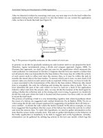
4.4 AP clustering algorithm
In this subsection, we present a two-stage heuristic algorithm for the AP clustering problem
to avoid combinatorial explosions. As an efficient heuristic, our algorithm finds an initial
solution by a greedy method, and improves it by the Variable Depth Search (VDS) method
that can enhance the search ability of a local search method by expanding neighbor states
flexibly (Yagiura et al., 1997). Our algorithm seeks the maximization of the network
performance with the number of clusters K. If any feasible solution cannot be found with
this number, our algorithm terminates after reporting the failure.
4.5 Check of number of clusters
First, the feasibility of the number of clusters K in the input is checked, because it has the trivial
upper and lower limits that can be given by other inputs of the problem. The upper limit K
max
is given by the number of GW candidates: K
max
= |X|. The lower limit K
min
is given by the
following equation to satisfy the cluster size constraint and the bandwidth constraint:
K
min
= max


N/P

,


N
∑
i=1
h
i
/H

(4)
where the ceiling function
x returns the smallest integer x or more. Then, if K < K
min
or
K
> K
max
, our algorithm terminates after reporting the feasible range of K.
4.5.1 Initial GW selection
In our algorithm, K APs are randomly selected as initial GWs among GW candidates in X
such that two selected APs are not adjacent to each other as best as possible. Starting from
these selected APs, the initial GW clusters are constructed sequentially. Then, the clusters
are iteratively improved by the VDS method. This AP clustering procedure is repeated by
min
(2N,
|X|
C
K
) times because initial GW APs are selected by different combinations, and the
best solution in terms of the cost function is selected as the final solution.
50
Wireless Mesh Networks

Access-Point Allocation Algorithms for Scalable
Wireless Internet-Access Mesh Networks
23
4.5.2 Greedy construction
Our algorithm generates an initial AP clustering by repeating the following procedure:
1. Sort the APs adjacent to the clustered APs in descending order of its load h
i
. If two or more
such APs have the same load, resolve this tiebreak in ascending order of the number of
incident links.
2. Apply the following procedure for each AP in step 1 from the top:
a. Select the cluster of its adjacent AP as a cluster candidate for the AP, if the following two
constraints are satisfied:
– the number of APs in the cluster is smaller than P for the cluster size constraint, and
– the total number of associated hosts in the cluster is H or smaller after the clustering
for the bandwidth constraint.
b. Cluster the AP as follows, if at least one cluster candidate is selected.
– Select this cluster candidate if only one candidate exists, or otherwise
– Select the cluster candidate that minimizes the cost function F
c
.
3. Repeat steps 1–2 until every AP is clustered or no more AP can be clustered.
4.5.3 GW update
If the selected AP in the sequential AP clustering (let AP
k
) is a GW candidate, the shortest
path is calculated from every AP in the same cluster to this AP passing through only APs in
this cluster, and the following GW cost function F
k
is computed:

F
k
= max(host(link
ij
)). (5)
If F
k
becomes smaller, AP
k
is selected as the new GW in the corresponding cluster.
4.5.4 Local search by VDS
Then, the initial AP clustering is improved iteratively by repeating the cluster changes of
multiple APs at the same time using the VDS method. VDS is a generalization of a local
search method, where the size of neighborhood is adaptively changed so that the algorithm
can effectively traverse the large search space while keeping the amount of computational
time reasonable. Actually, because each feasible state in this problem may have a different
size of its neighborhood that satisfies the four constraints, VDS is suitable for this problem.
In our VDS for the AP clustering, a simple move operation is repeatedly tried until no further
feasible operation is possible. Each move operation changes the cluster of an AP into a different
feasible one such that the cost function F
c
in (3) becomes minimum among the candidates.
Then, only the subsequence of the move operations resulting into the smallest cost function
are selected to be actually applied there, only if F
c
after these operations becomes equal to
or smaller than that of the previous state. If the cluster of any AP is not changed at one
iteration or the cost function has not been improved during R iterations (R
= 10 adopted in
this chapter), the state is regarded as the local minimum. Then, the hill-climbing procedure is

applied for the state to escape from it.
When the hill-climbing procedure is applied in T times (T
= 20), the local search by VDS is
terminated, and the best found solution is output as the final one. At this time, if an AP is
not clustered at all, our algorithm regards that the K clustering of the APs is impossible and
terminates after reporting the failure.
51
Access-Point Allocation Algorithms for Scalable Wireless Internet-Access Mesh Networks
24 Wireless Mesh Networks
In summary, one iteration of this stage consists of three steps: 1) the cluster change trial, 2)
the cluster change application, and 3) the hill-climbing. Here, we note that the unclustered
APs in the initial AP clustering may be clustered in VDS.
Cluster Change Trial: The cluster change trial repeats the cluster change of the AP that
satisfies the following three conditions until no more change is possible:
1. the AP has not been selected at this iteration,
2. the resulting clustering satisfies the constraints, and
3. the resulting clustering minimizes the cost function F
c
among candidates.
Cluster Change Application: The cluster change trial always changes the AP cluster
regardless of the increase of the cost function F
c
as long as it satisfies the constraints. Thus, F
c
may increase after some cluster changes. The cluster change application selects the subsequence
of the cluster changes that minimizes F
c
, and actually apply these cluster changes with the
GW update procedure in 4.5.3 to the current solution, only if F
c

becomes equal or smaller than
that of the previous iteration. If the cluster changes are actually applied, another iteration is
repeated from the cluster change trial.
Hill Climbing: The local search process using move operations in our VDS may be trapped
into a local minimum where the solution cannot be improved without the hill-climbing step.
In our algorithm, when either of the following two conditions is satisfied, the current state is
regarded as a local minimum, and the hill-climbing procedure is applied to escape from it:
1. no cluster change is applied at one iteration, or
2. F
c
has not been improved during R iterations (R = 10).
In the hill-climbing procedure, the following random cluster change operation is repeated until
the clusters of S APs are actually changed, or no more APs can be changed (S
= 10).
1. Enumerate any AP that satisfies the following three conditions for the random cluster
change:
a. it is not selected at this hill-climbing procedure,
b. it is located on the boundary between different clusters, and
c. its cluster change does not affect the connectivity of the other APs in the same cluster.
2. Randomly select one AP among them.
3. For this AP, find any cluster that can feasibly be changed into.
4. If such a cluster exists, change the cluster of this AP to a randomly selected cluster among
them.
5. Otherwise, remove the cluster of this AP.
4.6 Performance evaluation by simulations
In this subsection, we discuss the performance evaluation of the AP clustering algorithm
through network simulations using the WIMNET simulator. For this evaluation, the
compared algorithm in 4.6.1 is also implemented. In each simulated instance, the minimum
number of clusters such that each algorithm can find a feasible solution is given for the number
of clusters K respectively, because we regard the minimization of K as the first priority task in

the WIMNET design to reduce the installation and operation costs.
52
Wireless Mesh Networks
Access-Point Allocation Algorithms for Scalable
Wireless Internet-Access Mesh Networks
25
4.6.1 Compared algorithm
Within our knowledge, no algorithm has been reported for the same AP clustering problem in
this chapter. Therefore, as the most analogous algorithm to our problem, the Open/Close method
in (Prasad & Wu, 2006) has been implemented with some modifications for performance
comparisons with our algorithm, where it does not consider the cluster size constraint and
the distribution of associated hosts with APs. The procedure of this heuristic algorithm is
described as follows.
Initial AP clustering
1. Generate the sorted list of the APs in descending order of the maximum number of
associated hosts.
2. Select the first K APs in the list as GWs.
3. Assign the cluster to an unclustered AP that satisfies the following conditions:
– the AP is adjacent to an AP clustered to this GW cluster,
– the cluster size constraint is satisfied if added,
– the bandwidth constraint is satisfied if added, and
– the hop count (the number of hops between the AP and the GW) is minimized.
4. Repeat step 3 until no more AP can be assigned.
5. Calculate the sum of the hop count of every AP, if every AP is assigned a cluster, and save
it.
AP clustering Improvement
The initial clustering is iteratively improved by repeating the following three operations:
1. Close operation
a. Remove one GW randomly, and uncluster all the APs connected to this GW.
b. Go to Open operation.

2. Open operation
a. Select the first AP of the list in 4.6.1 as the GW that has not been selected.
b. If no more AP is selected in step a, output the best-found solution if found, or output
the error otherwise, and terminate the procedure.
c. Assign the GW cluster to an unclustered AP that satisfies the four conditions in 4.6.1.
d. Repeat step c until no more AP can be assigned.
e. If every AP is assigned a cluster, calculate the sum of the hop count of every AP, and
save it if the value is smaller than the best-found one. Return to Close operation.
f. Otherwise, go to Cluster adjustment.
3. Cluster adjustment
a. Assign the unassigned AP to one of the connectable GW clusters randomly.
b. If the cluster size constraint or the bandwidth constraint is not satisfied as the result of
the assignment in step a, APs in the cluster are unclustered one by one in ascending
order of the hop count until the constraint is satisfied. If every AP in the cluster except
the GW is unclustered but the constraint is not still satisfied, every unclustered AP is
resumed and the cluster assignment in step a is discarded.
53
Access-Point Allocation Algorithms for Scalable Wireless Internet-Access Mesh Networks
26 Wireless Mesh Networks
c. If every AP is assigned a cluster, calculate the sum of the hop count of every AP, and
save it if the value is smaller than the best-found one. Return to Close operation.
d. If no feasible solution is obtained after repeating Cluster adjustment in 300 times, abort
the procedure, and return to Close operation.
We note that the original Open/Close method assumes that each GW may have a
different bandwidth for communications to/from wired networks to the Internet. In our
implementation, we use the maximum number of associated hosts with an AP as this
bandwidth.
4.6.2 Simulations for different traffic patterns
In our first simulations, the performance of our algorithm is evaluated through simple
instances whose optimal solutions can be found easily, so that the optimality of our heuristic

algorithm can be verified. For this purpose, we adopt the simple network topology of
regularly allocated 24 (=6
× 4) APs, where each AP has wireless links with its four neighbor
APs on the left, right, top, and bottom sides. This grid topology has been often used in wireless
mesh network studies (Alicherry et al., 2006; Robinson & Knightly, 2007; Yan et al., 2008; Badia
et al., 2008; Ye et al., 2007). To generate non-uniform traffics using simple loads, 8 APs among
24 are associated with 10 hosts, and the remaining 16 APs are with 1 host, which means the
total of 96 hosts exist in the network. Then, by changing the locations of crowded APs in the
field, we prepare 10 instances of different traffic patterns.
As the input parameters of the algorithm, the cluster size limit P is set 6 and the bandwidth
size limit H is 24 where the lower limit on the number of clusters K
min
is 4. Every link is
assigned the same bandwidth s
ij
= 30Mbps, and every AP becomes a GW candidate with
X
= V for simplicity. The coefficients A = B = 1 are used for the cost function F
c
, because
our preliminary experiments using these instances observed no big difference in throughputs
when A and B were changed from 1 to 3. To avoid the bias in random numbers, the average
result among 10 runs using different random numbers is used in the evaluation for each
instance. As example instances in our first simulations, Figure 7 illustrates traffic patterns
and our clustering results with four clusters (K
= 4) for four instances among them, where a
black circle represents an AP associated with 10 hosts, and a white one represents an AP with
1 host. These results are actually optimum in these instances with the minimum number of
clusters and cost functions.
Figure 8 compares the average number of clusters among 10 runs between two algorithms

for each of 10 instances. Our algorithm (Proposal) always finds a feasible solution with
the minimum number of clusters for any instance, whereas the compared one (Comparison)
usually requires larger numbers. The reason may come from the fact that our algorithm seeks
a feasible better solution with the fixed number of clusters, whereas the compared one does
not explicitly minimize the number of clusters and may reduce it by chance through repeating
open/close operations.
Then, to evaluate the AP clustering results in terms of the network performance, the WIMNET
simulator is applied using the clustering results by both algorithms. Figure 9 compares the
average total throughput for each instance between two algorithms, where our algorithm
provides the larger throughput than the compared one by 24%–80% for any instance. Here,
we analyze the reason why our algorithm achieves at least 150Mbps. The total throughput
of one GW cluster is determined by the summation of the GW throughput and the maximum
communication throughput between APs in WIMNET. As shown in Fig. 8, the traffic load is
evenly distributed among four clusters in our algorithm, which gives the same throughput for
54
Wireless Mesh Networks
Access-Point Allocation Algorithms for Scalable
Wireless Internet-Access Mesh Networks
27
(a) instance 1 (b) instance 2
(c) instance 3 (d) instance 4
Fig. 7. Four traffic patterns and clustering results in first simulations.
every cluster. As a result, the total throughput of 150Mbps or more comes from the formula
of
((30 + Δ) ×4)Mbps where Δ represents the GW throughput by its associated hosts.
4.6.3 Simulations for verification of terms in cost function
The importance of each term in the cost function F
c
is verified through simulations using the
10 instances in 4.6.2. Figure 10 compares the average throughput among the four different

conditions for F
c
, where AB represents the result using both terms, A does the result using the
A-term only, B does the result using the B-term only, and None does the result without using
F
c
. This figure indicates that AB provides the best throughput in any simulated instance. Note
that all of them find the solution with the least number of clusters. Thus, we conclude that the
two terms in the cost function F
c
are necessary for finding the high quality AP clustering.
0.0
2.0
4.0
6.0
8.0
12345678910
Instance
# of clusters (K)
Proposal Comparison
Fig. 8. Average number of clusters for different traffic patterns.
55
Access-Point Allocation Algorithms for Scalable Wireless Internet-Access Mesh Networks
28 Wireless Mesh Networks
0.0
50.0
100.0
150.0
200.0
12345678910

Instance
Throughput (Mbps)
Proposal Comparison
Fig. 9. Average throughputs for different traffic patterns.
4.6.4 Simulations for different bandwidth limits
In our second simulations, the performance for different bandwidth limits is investigated for
instance 1 in Fig. 7. P is fixed with 8, and H is selected between 21 and 48, where K
min
is
3, 4, or 5. Figures 11 and 12 compare the average number of clusters and the average total
throughput, respectively. The number of clusters by our algorithm is always smaller than that
by the compared one, and the throughput is larger by 10%–183%. Generally, as the bandwidth
constraint becomes harder, both the number of clusters and the average throughput increase
except for H
= 21.
4.6.5 Simulations for different number of clusters
In our third simulations, the performance for different number of clusters is investigated using
instance 4 in Fig. 7, where P
= 12 and H = 48 are used, and the number of clusters K is changed
from 2 to 24. Figure 13 shows changes of the throughputs by two algorithms and the cost
function F
c
in our algorithm. This result indicates that as K increases until certain values, F
c
decreases and the throughput increases, and the throughput by our algorithm is always better
than that by the compared one when it is not saturated. The results confirm the effectiveness
of our algorithm for different number of clusters. Here, we note that the throughput are
saturated at certain values of K because the communication bandwidth between an AP and a
host (20Mbps in simulations) becomes the bottleneck.
0.0

50.0
100.0
150.0
200.0
12345678910
Instance
Throughput (Mbps)
AB A B None
Fig. 10. Performance comparison of F
c
with and without A or B-term.
56
Wireless Mesh Networks
Access-Point Allocation Algorithms for Scalable
Wireless Internet-Access Mesh Networks
29
0.0
2.0
4.0
6.0
8.0
48 44 40 36 32 28 24 23 22 21
H
# of clusters (K)
Proposal Comparison
Fig. 11. Average number of clusters for different bandwidth limits.
4.6.6 Simulations for random networks
In our fourth simulations, the performance for random networks with 50 APs is investigated
to evaluate our algorithm in more practical situations. The APs are randomly allocated on
the network field (500m

× 500m) such that the distance between any pair of APs is larger
than the minimum one (50m). Then, the wireless link is generated for any pair of APs within
the distance of 110m representing the wireless range in a free space. However, this wireless
link can be blocked by obstacles such as walls and furniture in indoor environments as target
fields for WIMNET. In order to consider the link failure stochastically, the following Waxman
method is adopted to generate the link randomly, which has been often used in network
studies (Waxman, 1988):
P
(u, v)=αe
−d/(βD)
(6)
where P
(u, v) is the probability of generating a link between AP
u
and AP
v
, α and β are
constants satisfying 0
< α, β ≤ 1(α = 0.9, β = 0.8), d is the distance between AP
u
and AP
v
,
D is the largest distance between two APs in the network (on average, D
= 647.6m). Then,
the maximum number of hosts associated with each AP is randomly generated between 1
and 10 such that the total number of them becomes 200, in order to consider various network
situations under the constant total load. As the constraints for GW clusters, P
= 6 and H = 25
are used for K

min
= 9.
By changing random numbers, 10 topologies are generated, and AP clusters are found by
applying both algorithms to each topology in 10 times. Then, the WIMNET simulator is
executed with each AP clustering in three times using different random numbers. As a result,
0.0
50.0
100.0
150.0
200.0
48 44 40 36 32 28 24 23 22 21
H
Throughput (Mbps)
Proposal Comparison
Fig. 12. Average throughputs for different bandwidth limits.
57
Access-Point Allocation Algorithms for Scalable Wireless Internet-Access Mesh Networks
30 Wireless Mesh Networks
0.0
50.0
100.0
150.0
200.0
2 4 6 8 1012141618202224
K
Throughput (Mbps)
0
20
40
60

Fc
Proposal Comparison Fc(Proposal)
Fig. 13. Average throughputs and F
c
for different number of clusters.
the average number of clusters and throughputs among the total of 30 trials for each of 10
topologies are evaluated in random network instances. Figure 14 illustrates two topologies
with AP clusters and GWs found by our algorithm. Figure 15 and 16 compare the simulation
results by both algorithms. The results show that our algorithm can find the AP clustering
with the least number of clusters, which provides the better performance than the compared
one for practical instances.
4.6.7 Simulations for load changes in random networks
In the AP clustering problem for WIMNET, the maximum number of associated hosts with
each AP is given as the input. Normally, the number of associated hosts with an AP is
frequently changing between 0 and this maximum number, because client hosts are often
moving and are randomly connecting to the Internet through WIMNET.
In order to evaluate the performance of our algorithm in such normal situations, one random
network instance is simulated when the number of associated hosts with each AP is changed
randomly between the minimum and the given maximum. To vary the load, this minimum
is changed from 1% of the maximum until reaching the maximum with the 1% interval.
Figure 17 compares the throughputs between our algorithm and the compared one under
100 different loads. The result shows that the AP clustering by our algorithm provides the
better throughput at any load than the compared one. Here, we note that if the maximum
load for an AP is changed, the AP clustering should be redesigned by applying our algorithm.
(a) instance 1 (b) instance 2
Fig. 14. Clustering results for two random networks.
58
Wireless Mesh Networks
Access-Point Allocation Algorithms for Scalable
Wireless Internet-Access Mesh Networks

31
0.0
5.0
10.0
15.0
12345678910
Instance
# of clusters (K)
Proposal Comparison
Fig. 15. Average number of clusters for random networks.
4.7 Related works
In this subsection, we introduce several related works to the AP clustering problem.
Unfortunately, none of them deal with the four constraints in this problem including the GW
cluster size constraint at the same time.
In (Aoun et al., 2006), Aoun et al. proposed a recursive dominating set algorithm based
on (Chvatal, 1979) to find a clustering such that the maximum hop count, or radius, inside
a cluster is smaller than the given limit. It first extracts a dominating set of the network, and
generates a graph composed of this set and the edges connecting the two APs with two hops in
the network. Then, it again extracts its dominating set, where any AP is connected with three
hops to an AP in this set. This recursive procedure is repeated until the hop count surpasses
the limit. This algorithm cannot generate clusters with an arbitrary hop count, and cannot
always satisfy the constraints of the cluster size, the bandwidth, and the GW.
In (Lakshmanan et al., 2006), Lakshmanan et al. presented a multiple GW association model of
allowing each host to be connected through more than one GWs to the Internet. They discuss
its benefits in capacity, fairness, reliability, and security with its challenges. They presented
the architecture using a super GW that controls the whole system, which can be a bottleneck,
and the algorithms for the GW association and the packet transmission scheduling, which are
just theoretical.
In (Li et al., 2007), Li et al. proposed a grid-based GW deployment method with a
linear programming for a feasible interference-free TDMA link scheduling to maximize the

throughput. By evaluating the throughput using the scheduling algorithm for every possible
combination of K grid points in the field, the best locations of K GWs are found. Their
0.0
100.0
200.0
300.0
400.0
12345678910
Instance
Throughput (Mbps)
Proposal Comparison
Fig. 16. Average throughputs for random networks.
59
Access-Point Allocation Algorithms for Scalable Wireless Internet-Access Mesh Networks
32 Wireless Mesh Networks
0.0
100.0
200.0
300.0
50 100 150 200
# of hosts
Throughput (Mbps)
Proposal Comparison
Fig. 17. Throughput changes for different numbers of hosts.
method can be extended to multi-channel and multi-radio networks. However, it assumes
impractical TDMA operations for wireless mesh networks. Furthermore, it does not consider
the constraints of the bandwidth, the cluster size, and the connection.
In (Park et al., 2006), Park et al. proposed a mesh router discovery scheme, and a
QoS-driven mesh router selection mechanism for the dynamic GW selection by the traffic
load. In (Nandiraju et al., 2006), Nandiraju et al. proposed a dynamic GW selection method

for load balancing among multiple GWs. Unfortunately, it does not consider interference.
These methods do not intend the allocation of GWs.
In (Hsiao & Kung, 2004), Hsiao et al. proposed a multiple network composition method with
the same channel by using directional antennas. In their method, a lot of APs are necessary
in the field so that each host can select its associated AP from multiple candidates for load
balancing.
In (Huang et al., 2006), Huang et al. investigated AP deployments for intelligent
transportation systems (ITS). They proposed an optimization algorithm of a mixed-integer
nonlinear programming to determine the optimal number of APs in a cluster and the best cell
radius for each AP. Because their proposal targets ITS, each cluster is composed of arrayed
APs and the first AP becomes the GW.
In (Alicherry et al., 2006), Alicherry et al. formulated the joint problem of the channel
assignment, the routing, and the scheduling for a special case of the wireless mesh
network where every link activation was synchronously controlled by a single global clock,
and presented its approximation algorithm that guarantees the order of approximation.
Unfortunately, the realization of the synchronous wireless mesh network is very hard, and
the superiority is actually not clear to the conventional asynchronous one. Furthermore, it
assumes that every AP has the same number of associated hosts.
In (Denko, 2008), Denko studied the wireless mesh network with mobile Internet GWs using
a multi-path routing scheme to increase the reliability and performance. However, the mobile
GW is not practical because the wired connection to the Internet is static. Furthermore, the
network may not work properly if the traffic of every router increases, because each router
selects one route by the amount of its traffic.
In (Tokito et al., 2009), Tokito et al. proposed a routing method for multiple GWs in
wireless mesh networks, called the GW load balanced routing (GLBR). GLBR reduces loads
of congested GWs by changing the GW of a leaf node in the routing tree one by one, such that
the new GW decreases the variance of loads at GWs and the length of the detouring path is
shorter than the threshold. The initial routing tree is found by the shortest path algorithm.
They show the advantage of their proposal over the shortest path routing in simulations.
60

Wireless Mesh Networks
Access-Point Allocation Algorithms for Scalable
Wireless Internet-Access Mesh Networks
33
However, because this algorithm can change the path for only one leaf node at one time, it
can be easily trapped into a local minimum where simultaneous changes of multiple paths
are often necessary to escape from.
In (Ito et al., 2009), Ito et al. studied a method of distributing traffics among multiple GWs
on a session by session basis in wireless mesh networks. Their method first estimates the
throughput for each GW from the traffic volume around there and the hop count, and then,
selects the GW expecting the highest throughput. Through simulations using the network
simulator ns-2, they show the effectiveness of their proposal by comparing the throughput and
the fairness between the proposed session-distribution method and the packet-distribution
method.
4.8 Conclusion
This section presented the AP clustering algorithm composed of the greedy method and the
variable depth search method. The effectiveness was verified through network simulations
using the WIMNET simulator, where the comparisons of the number of clusters and
throughputs with an existing algorithm confirmed the superiority of our algorithm. The
future works may include simulations with more realistic situations, the development of the
distributed version of the AP clustering algorithm, and experiments using real networks.
5. References
Akyildiz, I. F., Wang, X. & Wang, W. (2005). Wireless mesh networks: a survey, Comput.
Network. ISDN Syst. 47(4): 445–487.
Alicherry, M., Bhatia, R. & Li, L. (2006). Joint channel assignment and routing for throughput
optimization in multiradio wireless mesh networks, IEEE J. Select. Area. Commun.
24(11): 1960–1971.
Aoun, B., Boutaba, R., Iraqi, Y. & G, K. (2006). Gateway placement optimization in wireless
mesh networks with qos constraints, IEEE J. Select. Area. Commun. 24(11): 2127–2136.
Badia, L., Etra, A., Lenzini, L. & Zorzi, M. (2008). A general interference-aware framework

for joint routing and link scheduling in wireless mesh networks, IEEE J. Network
22(1): 32–38.
Bahri, A. & Chamberland, S. (2005). On the wireless local area network design problem with
performance guarantees, Comput. Networks 48: 856–866.
Beuran, R., Nakata, J., Okada, T., Nguyen, L. T., Tan, Y. & Shinoda, Y. (2008). A
multi-purpose wireless network emulator: Qomet, Proc. Int. Conf. Advanced Inform.
Network. Applications (AINA2008).
Chandra, R., Qiu, L., Jain, K. & Mahdian, M. (2004). Optimizing the placement of internet
taps in wireless neighborhood networks, Proc. Int. Conf. Network Protocols (ICNP),
pp. 271–282.
Chvatal, V. (1979). A greedy heuristic for the set-covering problem, Math. Oper. Res.
4(3): 233–235.
Cisco Systems, Inc. (2003). Cisco aironet 1200 series access points,’ product data sheet.
Clark, B. N. & Colbourn, C. J. (1990). Unit disk graphs, Discrete Mathematics 86: 165–177.
de la Roche, G., Rebeyrotte, R., JaffrRunser, K. & Gorce, J M. (2006). A qos-based fap criterion
for indoor 802.11 wireless lan optimization, Proc. IEEE Int. Conf. Commun. (ICC2006),
pp. 5676–5681.
Denko, M. K. (2008). Using mobile internet gateways in wireless mesh networks, Proc.
Advanced Inform. Network. Applications (AINA), Vol. 1, pp. 1086–1092.
61
Access-Point Allocation Algorithms for Scalable Wireless Internet-Access Mesh Networks
34 Wireless Mesh Networks
Farag, T., Funabiki, N. & Nakanishi, T. (2009). An access point allocation algorithm for indoor
environments in wireless mesh networks, IEICE Trans. Commun. E92-B(3): 784–793.
Faria, D. B. (2005). Modeling signal attenuation in ieee 802.11 wireless lans - vol. 1, Tech. Report
TR-KP06-0118, Kiwi Project, Stanford Univ. .
Funabiki, N., Nakanishi, T., Hassan, W. & Uemura, K. (2007). A channel configuration
problem for access-point communications in wireless mesh networks, Proc. IEEE Int.
Conf. Networks (ICON).
Funabiki, N., Uemura, K., Nakanishi, T. & Hassan, W. (2008). A minimum-delay routing

tree algorithm for access-point communications in wireless mesh networks, Proc. Int.
Conf. Research Innovation Vision for the Future (RIVF-2008), pp. 161–166.
Garey, M. R. & Johnson, D. S. (1979). Computers and intractability: A guide to the theory of
np-completeness.
Gast, M. S. (2002). 802.11 wireless networks - the definitive guide.
Gupta, G. & Younis, M. (2003). Fault-tolerant clustering of wireless sensor networks, Proc.
IEEE Wireless Commun. Networking Conf. (WCNC), Vol. 3, pp. 1579–1584.
Hassan, W., Funabiki, N. & Nakanishi, T. (2010). Extensions of the access point allocation
algorithm for wireless mesh networks, IEICE Trans. Commun. E93-B(6): 1555–1565.
Hsiao, P H., Hwang, A., Kung, H. T. & Vlah, D. (2001). Load-balancing routing for wireless
access networks, Proc. IEEE Infocom, pp. 986–995.
Hsiao, P H. & Kung, H. T. (2004). Layout design for multiple collocated wireless mesh
networks, Proc. Vehicular Technology Conf. (VTC), Vol. 5, pp. 3085–3089.
Huang, J H., Wang, L C. & Chang, C J. (2006). Wireless mesh networks for intelligent
transportation systems, Proc. Systems, Man and Cybernetics (SMC), Vol. 1, pp. 625–630.
Ito, M., Shikama, T. & Watanabe, A. (2009). Proposal and evaluation of multiple gateways
distribution method for wireless mesh network, Proc. Int. Conf. Ubiquitous Inform.
Manage. Commun. (ICUIMC), pp. 18–25.
Kato, H., Funabiki, N. & Nakanishi, T. (2007). Throughput measurements under various
contention window size in wireless mesh networks, IEICE Tech. Report, NS2007-115
pp. 55–60.
Kato, H., Nomura, Y., Funabiki, N. & Nakanishi, T. (2006). An experimental result of
communication bands for a wireless mesh network, IEICE Tech. Report, NS2006-139
pp. 5–8.
Kouhbor, S., Ugon, J., Mammadov, M., Rubinov, A. & Kruger, A. (2006). Nonsmooth
optimization for the placement of access points to enhance security in wlan.
Kouhbor, S., Ugon, J., Rubinov, A., Kruger, A. & Mammadov, M. (2006). Coverage in wlan
with minimum number of access points, Proc. IEEE Vehi. Tech. Conf. (VTC 2006),
pp. 1166–1170.
Lakshmanan, S., Sundaresan, K. & Sivakumar, R. (2006). On multi-gateway association

in wireless mesh networks, Proc. IEEE Workshop. Wireless Mesh Networks (WiMesh),
pp. 64–73.
Lee, Y., Kim, K. & Choi, Y. (2002). Optimization of ap placement and channel assignment in
wireless lans, Proc. Work. Wireless Local Networks.
Li, F., Wang, Y. & Li, X Y. (2007). Gateway placement for throughput optimization in wireless
mesh networks, Proc. IEEE Int. Conf. Commun. (ICC), pp. 4955–4960.
Li, J., Jannotti, J., Couto, D. S. J. D., Karger, D. R. & Morris, R. (2000). A scalable location service
for geographic ad hoc routing, Proc. Int. Conf. Mobile Comput. Network. (MobiCom),
pp. 120–130.
62
Wireless Mesh Networks
Access-Point Allocation Algorithms for Scalable
Wireless Internet-Access Mesh Networks
35
Lichtenstein, D. (1982). Planar formulae and their uses, Siam J. Comput 11: 329–343.
Nagy, L. & Farkas, L. (2000). Indoor base station location optimization using genetic
algorithms, IEEE Int. Symp. Personal, Indoor, and Mobile Radio Commun. (PIMRC),
Vol. 2, pp. 843–846.
Naidoo, K. & Sewsunker, R. (2007). 802.11 mesh mode provides rural coverage at low cost,
Proc. AFRICON 2007.
Nandiraju, D., Santhanam, L., Nandiraju, N. & Agrawal, D. P. (2006). Achieving load
balancing in wireless mesh networks through multiple gateways, Proc. Mobile Adhoc
and Sensor Systems (MASS), pp. 807–812.
Pal, M., Tardos, E. & Wexler, T. (2001). Facility location with nonuniform hard capacities, Proc.
IEEE Symp. Found. Comput. Science, pp. 329–338.
Pan, H. J. & Keshav, S. (2006). Detection and repair of faulty access points, Proc. IEEE Wireless
Commun. Networking Conf. (WCNC), pp. 532–538.
Park, B N., Lee, W., Ahn, S. & Ahn, S. (2006). Qos-driven wireless broadband home
networking based on multihop wireless mesh networks, IEEE Trans. Consumer
Electronics 52(4): 1220–1228.

Prasad, R. & Wu, H. (2006). Gateway deployment optimization in cellular wi-fi mesh
networks, J. Networks 1(3): 31–39.
Proxim Co. (2003). A detailed examination of the environmental and protocol parameters that
affect 802.11g network performance.
URL: />Ramamurthy, R., Bogdanowicz, Z., Samieian, S., Saha, D., Rajagopalan, B., Sengupta, S.,
Chauduri, S. & Bala, K. (2001). Capacity performance of dynamic provisioning in
optical networks, J. Lightwave Technol. 19: 40–48.
Raniwala, A., Gppalan, K. & Chiueh, T. (2005). Architecture and algorithms for an ieee
802.11-based multi-channel wireless mesh networks, Proc. IEEE Infocom, Vol. 3,
pp. 2223–2234.
Rappaport, T. S. (1996). Wireless communications - principles and practice.
Robinson, J. & Knightly, E. W. (2007). A performance study of deployment factors in wireless
mesh networks, Proc. Inform. Commun.(INFOCOM), pp. 2054–2062.
Robinson, J., Uysal, M., Swaminathan, R. & Knightly, E. (2008). Adding capacity points to a
wireless mesh network using local search, Proc. IEEE Infocom.
Sharma, A., Raghavenda, R., Puttaswamy, K., Lundgren, H., Almeroth, K. & Belding-Ro,
E. (2005). Experimental characterization of interference in a 802.11g wireless mesh
network, Tech. Paper, Univ. California Santa Barbara .
Tajima, S., Funabiki, N. & Higashino, T. (2010). A wds clustering algorithm for wireless mesh
networks, IEICE Trans. Inform. Systems E93-D(4): 800–810.
Tokito, H., Sasabe, M., Hasegawa, G. & Nakano, H. (2009). Routing method for gateway load
balancing in wireless mesh networks, Proc. Int. Conf. Networks (ICN), pp. 127–132.
Varshney, U. & Malloy, A. D. (2006). Multilevel fault tolerance in infrastructure-oriented
wireless networks: framework and performance evaluation, Int. J. Network
Management 16: 351–374.
Waxman, B. M. (1988). Routing of multipoint connections, IEEE J. Select. Areas Commun.
6(9): 1617–1622.
Wu, T W. & Hsieh, H Y. (2007). Interworking wireless mesh networks: performance
characterization and perspectives, Proc. IEEE Global Telecom. Conf. (GLOBECOM),
pp. 4846–4851.

63
Access-Point Allocation Algorithms for Scalable Wireless Internet-Access Mesh Networks