Wireless Mesh Networks

14
perturbations. The SPWC-PMMUP coordinates the optimal TPM executions in UCGs. The
key attributes are that the SPWC-PMMUP scheme minimizes the impacts of: (i) queue
perturbations, arising between energy and packet service variations, and (ii) cross-channel
interference problems owing to the violation of orthogonality of multiple channels by wireless
fading. The proposed TPM scheme is discussed in the following sections: 4.1 and 4.2.

Internet Protocol (IP) and Upper layers
in the Network Protocol Stack
Singularly Perturbed and Weakly
Coupled-PMMUP module
(SPWC PMMUP)
Neighbour
communication
power selection -
channel state’s
(NCPS) table
Address
Resolution
Protocol (ARP)
MAC and NIC 1
Channel 1
MAC and NIC i
MAC and NIC N
Channel l
Channel L
. . .
. . .

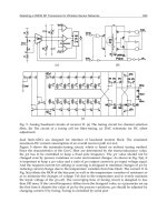
Fig. 5. Singularly-perturbed weakly-coupled PMMUP architecture
4.1 Timing phase structure
The SPWC-PMMUP contains L parallel channel sets with the virtual timing structure shown
in Fig. 6. Channel access times are divided into identical time-slots. There are three phases in
each time-slot after slot synchronization. Phase I serves as the channel probing or Link State
Information (LSI) estimation phase. Phase II serves as the Ad Hoc traffic indication message
(ATIM) window which is on when power optimization occurs. Nodes stay awake and
exchange an ATIM (indicating such nodes’ intention to send the queue data traffic) message
with their neighbours (Wang et al., 2006). Based on the exchanged ATIM, each user
performs an optimal transmission power selection (adaptation) for eventual data exchange.
Phase III serves as the data exchange phase over power controlled multiple channels.
Phase I: In order for each user to estimate the number of active links in the same UCG,
Phase I is divided into M mini-slots. Each mini-slot lasts a duration of channel probing time
T
cp
, which is set to be large enough for judging whether the channel is busy or not. If a link
has traffic in the current time-slot, it may randomly select one probe mini-slot and transmit a
busy signal. By counting the busy mini-slots, all nodes can estimate how many links intend
to advertise traffic at the end of Phase I. Additionally, the SPWC-PMMUP estimates: the
inter channel interference (i.e., weak coupling powers), the intra-UCG interference (i.e., the
strong coupling powers), the queue perturbation and the LSI addressed in (Olwal et al.,

Optimal Control of Transmission Power Management in Wireless Backbone Mesh Networks

15

Fig. 6. The virtual SPWC-PMMUP timing structure
2009
a). It should be noted that the number of links intending to advertise traffic, if not zero,
could be greater than the observed number of busy mini-slots. This occurs because there

might be at least one link intending to advertise traffic during the same busy mini-slot.
Denote the number of neighbouring links in the same UCG intending to advertise traffic at
the end of Phase I as
n . Given
M
and n , the probability that the number of observed busy
mini-slots equals
m
, is calculated by

()
1
1
,,
1
1
r
Mn
mm
PMnm
nM
M
−
⎛⎞⎛ ⎞
⎜⎟⎜ ⎟
−
⎝⎠⎝ ⎠
=
+−
⎛⎞

⎜⎟
−
⎝⎠
(12)
Let
n
remain the same for the duration of each time-slot t . Denote the estimate of the
number of active links as
(
)
ˆ
nt and the probability mass function (PMF) that the number of
busy mini-slots observed in the previous time-slot equals
k as
(
)
k
f
t . Denote
(
)
mt as the
number of the current busy mini-slots. The estimate
(
)
ˆ
nt
is then derived from the
estimation error process as,


()
()
()
()
()()
{
}
ˆ
arg min , ,
nn
rk
kmt kmt
nmt
nt P Mnk f t
==
≥
=−
∑∑
, (13)
where
()
k
f
t from one time-slot to other is updated as
Wireless Mesh Networks

16

()
()

(
)
() ()
()
()
()() ()
11,
11,
k
k
m
tft kmt
ft
tft t kmt
α
αα
⎧
−− ≠
⎪
=
⎨
−−+=
⎪
⎩
, (14)
and
(
)
(
)

(
)
,0 1tt
αα
<< is the PMF update step size, which needs to be chosen appropriately
to balance the convergence speed and the stability. Of course, selecting a large value of
M

when Phase I is adjusted to be narrower will imply short
c
p
T periods and negligible delay
during the probing phase. Short channel probing phase time allows time for large actual
data payload exchange, consequently improving network capacity.
Phase II: In this phase, the TPM problem and solution are implemented. Suppose the
number of busy mini-slots is non-zero; then the SPWC-PMMUP module performs a power
optimization following the
p
−
persistent algorithm or back-off algorithm (Wang et al.,
2006). Otherwise, the transmission power optimization depends on the queue status only
(i.e., the evaluation of the singular perturbation of the queue system). The time duration of
the power optimization is denoted as
2
T and the minimal duration to complete power
optimization as a function of the number of participating users in a p-persistent CSMA, is
denoted as
(
)
,

succ
Tnp
∗
. The transmission power optimization time allocation
2
T is then
adjusted according to

(
)
{
}
ˆ
max
22
1
min , ,
n
succ
n
TT Tnp
ϑ
∗
=
=
∑
, (15)
where
max
2

T is the power allocation upper bound time,
ϑ
is the power allocation time
adjusting parameter and
ˆ
n
is the estimated number of actively interfering neighbour links
in the same UCG. The steady state medium access probability
p in terms of the minimal
average service time can be computed as (Wang et al., 2006),

()
{
}
01
ar
g
min ,
succ
p
p
Tn
p
∗
<<
= . (16)
It should be noted that due to energy conservation,
1
T
and

2
T
should be short enough and
the optimal
p
∗
can be obtained from a look up table rather than from online computation.
The TPM solution is then furnished according to section 4.2.
Phase III: Data is exchanged by NICs over parallel multiple non-overlapping channels
within a time period of
3
T . The RTS/CTS are exchanged at the probe power level which is
sufficient in order to resolve collisions due to hidden terminal nodes. Furthermore, the
optimal medium access probability
p
∗
resolves RTS/CTS collisions. After sending data
traffic to the target receiver, each node may determine the achievable throughput according to,

()
()
()
,
,2 , , 3
1
,,,
L
swp
ldata
rswpswpjldataldata

i
l
ij
L
Th t P n p T j P n p T
t
=
⎧
⎫
⎧
⎫
⎪
⎪⎪⎪
=×
⎨
⎨⎬⎬
⎪
⎪⎪⎪
⎩⎭
⎩⎭
∑∑∑

GG G G
. (17)
Here, L

is the application/data packet length and t is the length of one virtual time-slot
which equals
123
TTT

+
+
. Denote
2
(,,)
swp
swp swp
i
PnpT
G
G
as the SPWC based probability that i
actively interfering links successfully exchange ATIM in Phase II, given the number of links
intending to advertise traffic as,
sw
p
n
G
and the medium access probability sequence as,
sw
p
p
G

Optimal Control of Transmission Power Management in Wireless Backbone Mesh Networks

17
during time
2
T period. Denote

(
)
,
,,3
,,
ldata
ildataldata
Pn
p
T
G
G
as the probability that i data packets
are successfully exchanged on channel l in Phase III, given the number sequence
,ldata
n
G
and
the medium access probability sequence as
,ldata
p
G
during time
3
T period. The computations
of such probabilities have been provided in (Li et al., 2009). If several transmissions are
executed, then the average throughput performance can be evaluated. The energy efficiency
in joules per successfully transmitted packets then becomes

(

)
()
/s
eff
o
p
timal transmission
p
ower
p
er node watts
E
average throughput per node packets
= . (18)
It should be noted that a high throughput implies a low energy-efficiency for a given
optimal power level, because of the high data payload needed to successfully reach the
intended receiver within a given time slot. The use of an optimal power level is expected to
yield a better spectrum efficiency and throughput measurement balance.
4.2 Nash strategies
The optimal solution to the given problem (10) with the conflict of interest and simultaneous
decision making leads to the so called Nash strategies (Gajic & Shen, 1993)
1
, , , ,
iN
∗∗∗
uuu
satisfying

()
(

)
1
, , , , , 0
iiN
J
∗∗∗
uuux


()
(
)
1
, , , , , 0
iiN
J
∗∗
≤ uuux,
ii
∗
≠
uu, 1, ,iN
=
. (19)
Assumption 1: Each thi user has optimal closed-loop Nash strategies yielded by

(
)
(
)

ii
tt
ε
∗∗
=−uFx, 1, . . . ,iN
=
. (20)
Here, the decoupled
i
ε
∗
F is the regulator feedback gain with singular-perturbation and
weak-coupling components defined as

12
11 1
12

ii Ni
n
iiiNi
δδ δ
ε
εε ε
−− −
⎡⎤
=
∈ℜ
⎣⎦
FFF F, (21)

with
1
N
i
i
nn
=
=
∑
,
i
n is the size of the vector
i
x and
(
)
()
0
1
ij
ij
ij
δ
⎧
≠
⎪
=
⎨
=
⎪

⎩
.
Define the N-tuple discrete in time Nash strategies by

() ()
()
()
1
TT
ii iiiiiii
tt t
εεεεεεε
−
∗∗
=− =− +uFxRBPBBPAx, 1, . . . ,iN
=
, (22)
where
()
1
, ,
NN
F
εε
∗∗
∈FF and N-tuple
(
)
i
t

∗
u , form a soft constrained Nash Equilibrium
represented as

()
(
)
() ()
1
, , , 0 0 0
T
iN i
J
εε ε
∗∗
=Fx F xx x Px . (23)
Wireless Mesh Networks

18
Here, the decoupled
i
ε
P is a positive semi-definite stabilizing solution of the discrete-time
algebraic regulator Riccati equation (DARRE) with the following structure:

1
2
1
1212 1
1

1
212 2 2
2
1
12
.
.

.
i
i
iN
iii iNiN
i
T
T
ii i iNiN
i
ii
TT
iN i N iN i N iN
nn
δ
δ
εε
δ
εε ε
εε ε
εε ε
−

−
−
×
⎡
⎤
⎢
⎥
⎢
⎥
==
⎢
⎥
⎢
⎥
⎢
⎥
⎣
⎦
∈ℜ
PP P
PPP
PP
PP P
, (24)
where the DARRE is given by

()
1
TT T T T
ε

ε ε εε ε εεε ε εεε εε ε
−
=+ − +P D D A PA A PB R B PB B PA , (25)
with
()
1

N
=RdiagR R ,
(
)
()
()
11 12 12 1 1
21 21 22 2 2
11 22




NN
NN
NN NN NN
nn
ε
εε ε
εεε
ε
εε
×

⎡
⎤
⎢
⎥
⎢
⎥
=
⎢
⎥
⎢
⎥
⎢
⎥
⎣
⎦
∈ℜ
DD D
DD D
D
DD D

.
It should be noted that the inversion of the partitioned matrices
T
ε
εεε
+RBPB in (25) will
produce numerous terms and cause the DARRE approach to be computationally very
involved, even though one is faced with the reduced-order numerical problem (Gajic &
Shen

, 1993). This problem is resolved by using bilinear transformation to transform the
discrete-time Riccati equations (DARRE) into the continuous-time algebraic Riccati equation
(CARRE) with equivalent co-relation.
The differential game Riccati matrices
i
ε
P satisfy the singularly-perturbed and weakly-
coupled, continuous in time, algebraic Regulator Riccati equation (SWARREs) (Gajic & Shen,
1993; Sagara et al., 2008) which is given below,
(
)
1
, , , ,
iiN
εε ε
Ω=PPP

11
T
NN
i
jj jj
i
jj
ji ji
ε
εεε εεεε
==
≠≠
⎛⎞⎛⎞

⎜⎟⎜⎟
−+−
⎜⎟⎜⎟
⎜⎟⎜⎟
⎝⎠⎝⎠
∑∑
PA SP A SP P

1
N
iii i
jj
i
jj
j
ji
ε
εε ε εε
ε
=
≠
−+
∑
PSP PS P
T
iii ii
εεε εε
+
Μ+ =PPDD 0, (26)
where

1 T
iiiii
ε
εε
−
=SBRB
, 1, ,iN
=
.
11T
i
jjjj
i
jjj j
ε
ε
−−
=SBRRRB, 1, . . .,iN
=
.
1
ii
ε
εεε
−
Μ= Θ
w
W
W , 1, ,iN
=

.
Optimal Control of Transmission Power Management in Wireless Backbone Mesh Networks

19
By substituting the partitioned matrices of
ε
A ,
i
ε
S ,
i
j
ε
S ,
i
ε
Μ
,
i
ε
D , and
i
ε
P into SWARRE
(26), and by letting
0
w
ε
=
and any 0

s
ε
≠
, then simplifying the SWARRE (26), the following
reduced order (auxiliary) algebraic Riccati equation is obtained,

(
)
0
TT
ii ii ii ii ii ii ii ii ii ii
+
−−Μ+ =PA A P P S P D D , (27)

where
1 T
ii ii ii ii
−
=SBRB and
1 T
ii ii ii ii
−
Μ= Θ
W
W , and
ii
P , 1, . . .,iN
=
is the 0-order
approximation of

i
ε
P when the weakly-coupled component is set to zero, i.e., 0
w
ε
= . It
should be noted that a unique positive semi-definite optimal solution
*
i
ε
P exists if the
following assumptions are taken into account (Mukaidani, 2009).
Assumption 2: The triples
ii
A ,
ii
B and
ii
D , 1, ,iN
=
, are stabilizable and detectable.
Assumption 3: The auxiliary (27) has a positive semidefinite stabilizing solution such that
ii ii ii
=−AASP

is stable.
4.3 Analysis of SPWC-PMMUP optimality
Lemma 1: Under assumption 3 there exists a small constant
∗
∂

such that for all
()
(
)
0,t
ε
∗
∈∂

,
SWARRE admits a positive definite solution
i
ε
∗
P represented as
(
)
(
)
iii
Ot
εε
ε
∗
==+PPP , 1, ,iN
=
and
()
ws
t

ε
εε
=

,

(
)
(
)
(
)
0 0
ii
Ot
ε
=+block diag P

. (28)

Proof: This can be achieved by demonstrating that the Jacobian of SWARRE is non-singular
at
(
)
0t
ε
=

and its neighbourhood, i.e.,
(

)
0t
ε
→+ . Differentiating the function
(
)
(
)
1
, , ,
iN
t
ε
ε
ε
Ω PP

with respect to the decoupled matrix
i
ε
P produces,
()
()
1
, , ,
T
ii i N
i
vec t
vec

εε
ε
ε
∂
=Ω
∂
JPP
P

ii
TT
ii n n ii
II
=
Δ⊗ + ⊗Δ.

()
()
1
,, ,
T
ij i N
ij
vec t
vec P
εε
ε
∂
=Ω
∂

JPP

,

(
)
(
)
,
ii
TT
ji ijijj n n ji ijijj
II
εε εε εε ε ε
εε
=− − ⊗ − ⊗ −SP SP SP SP

(29)

where ij≠ , 1, ,jN= and
1
N
jj
ii
j
ij
ε
εε εε
=
≠

Δ= − +Μ
∑
ASP P
.
Exploiting the fact that ( ( ))
ji
Ot
εε
ε
=
SP

for
ij
≠
, the Jacobian of SWARRE with
(
)
0t
ε
→+


can be verified as
()
11
ˆ

NN
=ΔΔJblockdiag ,

(
)
ˆˆ
=
J
block diag J J .
Wireless Mesh Networks

20
Since the determinant of
ii ii ii ii ii ii
Δ
=− +ASPMPwith
(
)
0t
ε
=

is non-zero by following
assumption 3 for all
1, ,iN
=
, thus det 0
≠
J i.e., J is non-singular for
(
)
0t
ε

=

. As a
consequence of the implicit function theorem,
ii
P is a positive definite matrix at
(
)
0t
ε
=


and for sufficiently small parameters
()
(
)
0,t
ε
∗
∈
∂

, one can conclude that (())
iii
POt
ε
ε
=+P



is also a positive definite solution.
Theorem 1: Under assumptions 1-3, the use of a soft constrained Nash equilibrium
(
)
()
(
)
()
kk
ii
tt
ε
∗∗
=−uFx results in the following condition.

() ()
()
(
)
()
(
)
(
)
21
1
1
, , , 0 , , , 0
k

kk
iiN
N
JJO
ε
∗∗
∗∗ +
≈+uux uux

. (30)
Proof:
Due to space constraints, we merely outline the proof. A detailed related analysis can
be found in (Mukaidani, 2009; Sagara et al., 2008).
If the iterative strategy is
(
)
()
(
)
()
kk
ii
tt
ε
∗∗
=−uFx
then the value of the cost function is given by

() ()
()

(
)
() ()
1
,. . . , , 0 0 0
kk
T
ii
N
J
ε
∗∗
=uuxxYx
, (31)
where
i
ε
Y
is a positive semi-definite solution of the following algebraic Riccati equation
() ()
11
T
NN
kk
jj
i
jj
i
jj
ji ji

ε
εε εεε
εε
==
≠≠
⎛⎞⎛⎞
−+−
⎜⎟⎜⎟
⎝⎠⎝⎠
∑∑
YA SP A SP Y

(
)
(
)
(
)
(
)
1
N
kkkk
T
j
iii ij i ii
jjii
ji
εεε ε ε εε
εεεε

ε
=
≠
+
Μ+ − + =
∑
YY PSPPSPDD0. (32)
Let
iii
ε
εε
=−ZYP
; then subtracting SWARRE (26) from (32) satisfies the following equation
() ()
()
(
)
1
N
k
kkT
iiijj
j
j
ji
εε ε ε εε ε
ε
=
≠
++ −

∑
ZA A Z PS P P
()
(
)
() ()
(
)
11
NN
kkk
jji ijjijj
jjj
jj
ji ji
εεε εεεε
εεε
ε
==
≠≠
⎡
⎤
⎢
⎥
+− + −
⎢
⎥
⎢
⎥
⎣

⎦
∑∑
PPSP PSP PSP
()
(
)
()
(
)
0
kk
iii
ii
εεε
εε
+
−−=PPSPP , (33)
where
()
() () ()
(
)
1
N
kk k
k
jiii
ji i
j
εε ε ε εε

εε ε
=
=− + + −
∑
AA SPMPMPP. Suppose
()
(
)
2
k
k
i
i
O
ε
ε
ε
−≈PP

,
(i.e., has a quadratic rate of convergence); then from the proof of theorem 1, one can have,

()
()
(
)
()
(
)
(

)
21
ˆˆ
0
k
T
ii iiii
OO O
εε εεεε
θεε ε
+
=
+++ + + =ZZJ J ZZMZ
 
, (34)
where
()
(
)
21
k
O
θε
+
=0

and
()
11
ˆ


NN
=ΔΔJblockdiag with
(
)
ii ii ii ii ii
Δ= − −ASMP

[258]. Thus, let
(
)
21
k
i
O
ε
ε
+
−≤Z0

and from the cost function definition it is evident that:
Optimal Control of Transmission Power Management in Wireless Backbone Mesh Networks

21
(
)
(
)
(
)

(
)
(
)
(
)
00 0000
TTT
iii
εεε
=−xZx xYx xPx

() ()
()
(
)
()
(
)
1
1
, , , 0 , , , 0
kk
iiN
N
JJ
∗∗
∗∗
=−uuxuux


(
)
21

k
O
ε
+
≤

. (35)
5. Simulation tests and results
5.1 Simulation tests
The efficiency of the proposed model and algorithm was studied by means of numerical
examples. The MATLAB
TM
tool was used to evaluate the design optimization parameters,
because of its efficiency in numerical computations. The wireless MRMC network being
considered was modelled as a large scale interconnected control system. Upto 50 wireless
nodes were randomly placed in a 1200 m by 1200 m region. The random topology depicts a
non-uniform distribution of the nodes. Each node was assumed to have at most four NICs
or radios, each tuned to a separate non-overlapping UCG as shown in Fig. 7. Although 4
radios are situated at each node, it should be noted that such a dimension merely simplifies
the simulation. The higher dimension of radios per node may be used without loss of
generality. The MRMC configurations depict the weak coupling to each other among
different non-overlapping channels. In other words, those radios of the same node operating
on separate frequency channels (or UCGs) do not communicate with each other. However,
due to their close vicinity such radios significantly interfere with each other and affect the
process of optimal power control. The ISM carrier frequency band of 2.427 GHz-2.472 GHz
was assumed for simulation purposes only. Figure 7 illustrates the typical wireless network

scenario with 4 nodes, each with 4 radio-pairs or users able to operate simultaneously. The
rationale is to stripe application traffic over power controlled multiple channels and/or to
access the WMCs as well as backhaul network cooperation (Olwal et al., 2009
a).

NODE A
1
NODE B NODE C
NODE D
3
2
4
1
3
4
2
4
1
3
2 4
1
3
2
UCG # 1
UCG # 2
UCG # 3
UCG # 4
NIC
NIC
NIC

NIC
NIC
NIC
NIC
NIC
NIC
NIC
NIC
NIC
NIC
UCG # 3
UCG # 3"

Fig. 7. MRMC wireless network
Wireless Mesh Networks

22
5.2 Performance evaluation
In order to evaluate the performance of the singularly-perturbed weakly-coupled dynamic
transmission power management (TPM) scheme in terms of power and throughput, our
simulation parameters, additional to those in section 5.1, were outlined as follows: The
Distributed Inter Frame Space (DIFS) time = 50
s
μ
, Short Inter Frame Space (SIFS) time =
10
s
μ
and Back-off slot time = 20
s

μ
. The number of mini-slots in the probe phase, M = 20,
duration of probe mini-slot, T
pc
= 40 s
μ
and ATIM and power selection window adjustment
parameter,
ϑ
= 1.2-1.5 as well as a virtual time-slot duration consisting of probe, power
optimization and data packet transmission times,
t = 100 ms.
An arrival rate of
λ
packets/sec of packets at each queue was assumed. For each arriving
packet at the sending queue, a receiver was randomly selected from its immediate
neighbours. Each simulation run was performed long enough for the output statistics to
stabilize (i.e., sixty seconds simulation time). Each datum point in the plots represents an
average of four runs where each run exploits a different randomly generated network
topology. Saturated transmission power consumption and throughput gain performance
were evaluated. Saturation conditions mean that packets are always assumed to be in the
queue for transmission; otherwise, the concerned transmitting radio goes to doze/sleep
mode to conserve energy (i.e., back-off amount of time).
The following parameters were varied in the simulation: the number of active links
(transmit-receive radio-pairs) interfering (i.e., co-channel and cross-channel), from 2 to 50
links, the channels‘ availability, from 1 to 4 and the traffic load, from 12.8 packets/s to 128
packets/s. The maximum possible power consumed by a radio in the transmit state, the
receive state, the idle state and the doze state was assumed as 0.5 Watt, 0.25 Watt, 0.15 Watt
and 0.005 Watt, respectively. A user being in the transmitting state means that the radio at
the head of the link is in the transmit state while the radio at the tail of the link is in the

receive state. A user in the receive state, in the idle state, and in the doze state means that
both the radio at the head of the link and the radio at the tail of the link are in the receive
state, in the idle state, and in the doze state, respectively (Wang et al., 2006). In order to
evaluate the transmission power consumption, packets must be assumed to be always
available in all the sending queues of nodes. This is a condition of network saturation.
5.3 Results and disscussions
Figure 8 illustrates an average transmission power per node pair at steady state, versus the
number of active radios relative to the total number of adjacent channels. During each time
slot, each node evaluates steady state transmission powers in the ATIM phase. Average
transmission power was measured as the number of active radio interfaces was increased at
different values of the queue perturbations and the weak couplings of the MRMC systems.
An increase in the number of active interfaces results in a linear increase in the transmission
powers per node-pairs. At 80%, the number of radios relative to the number of adjacent
channels with
0.0001
sw
εεε
==
yields about 0.61%, 7.98%, 9.51% respectively, a greater
power saving than with
0.001
ε
=
, 0.01 and 0.1. This is explained as follows. Stabilizing a
highly perturbed queue system and strongly interfered disjoint wireless channels consumes
more source energy. Packets are also re-transmitted frequently because of high packet drop
rates. Retransmitting copies of previously dropped packets results in perturbations at the
queue system owing to induced delays and energy-outages.
Optimal Control of Transmission Power Management in Wireless Backbone Mesh Networks


23
A number of previously studied MAC protocols for throughput enhancement were
compared with the SPWC-PMMUP based power control scheme. The multi-radio
unification protocol (MUP) was compared with the SPWC-PMMUP scheme because the
latter is a direct extension of the former in terms of energy-efficiency. Both protocols are
implemented at the LL and with the same purpose (i.e., to hide the complexity of the
multiple PHY and MAC layers from the unified higher layers, and to improve throughput
performance). However, the MUP scheme chooses only one channel with the best channel
quality to exchange data and does not take power control into consideration. The power-
saving multi-radio multi-channel medium access control (MAC) (PSM-MMAC) was
compared with the SPWC-PMMUP scheme, because both protocols share the following
characteristics: they are energy-efficient, and they select channels, radios and power states
dynamically based on estimated queue lengths, channel conditions and the number of active
links. The single-channel power-control medium access control (POWMAC) protocol was
compared with the SPWC-PMMUP because both are power controlled MAC protocols
suitable for wireless Ad Hoc networks (e.g., IEEE 802.11 schemes). Such protocols perform
the carrier sensed multiple access with collision avoidance (CSMA/CA) schemes. Both
protocols possess the capability to exchange several concurrent data packets after the
completion of the operation of the power control mechanism. Both are distributed,
asynchronous and adaptive to changes of channel conditions.
Figure 9 depicts the plots for energy-efficiency versus the number of active links per square
kilometre of an area. Energy-efficiency is measured in terms of the steady state transmission
power per time slot, divided by the amount of packets that successfully reach the target
receiver. It is observed that low active network densities generally provide higher energy-
efficiency gain than highly active network densities. This occurs because low active network
densities possess better spatial re-use and proper multiple medium accesses. Except for low
network densities, the SPWC-PMMUP scheme outperforms the POWMAC, the power
saving multi-channel MAC (i.e., PSM-MMAC) and the MUP schemes. In low active network
density, a single channel power controlled MAC (i.e., POWMAC) records a higher degree of
freedom with spatial re-use. As a result, it indicates a low expenditure of transmission

power. As the number of active users increases, packet collisions and retransmissions
become significantly large. The POWMAC uses an adjustable access window to allow for a
series of RTS/CTS exchanges to take place before several concurrent data packet
transmissions can commence. Unlike its counterparts, the POWMAC does not make use of
control packets (i.e., RTS/CTS) to silence neighbouring terminals. Instead, collision
avoidance information is inserted in the control packets and is used in conjunction with the
received signal strength of these packets to dynamically bound the transmission power of
potentially interfering terminals in the vicinity of a receiving terminal. This allows an
appropriate selection of transmission power that ensures multiple-concurrent transmissions
in the vicinity of the receiving terminal. On the other hand, both SPWC-PMMUP and PSM-
MMAC contain an adjustable ATIM window for traffic loads and the LL information. The
ATIM window is maintained moderately narrow in order that less energy is wasted owing
to its being idle. Statistically, the simulation results indicated that for between 4 and 16 users
per deployment area, the POWMAC scheme was on average 50%, 87.50%, and 137.50%
more energy-efficient than the SPWC-PMMUP, PSM-MMAC and MUP, respectively.
However, between 32 and 50 users per deployment area, in the SPWC-PMMUP scheme,
yielded on average 14.58%, 66.67%, and 145.83% more energy efficiency than the POWMAC,
PSM-MMAC and MUP schemes, respectively.
Wireless Mesh Networks

24
0.2 0.4 0.6 0.8 1
0.2
0.25
0.3
0.35
0.4
0.45
0.5
SS trx. power in a 4 Channel node pair system

Average trx. power per node-pair (watts/slot)
# of radios relative to # of channels


ε
=0.0001
ε
=0.001
ε
=0.01
ε
=0.1

Fig. 8. Steady state transmission power versus relative number of radios per channel

4 8 16 32 50
0
0.02
0.04
0.06
0.08
0.1
0.12
Energy Efficiency
no. of active links per KM
2
Energy Efficiency(joules/packet)


MUP

SPWC-PMMUP
ε
=0.001
PSM-MMAC
POWMAC

Fig. 9. Energy-efficiency versus density of active links
Figure 10 depicts the performance of the network lifetime observed for the duration of the
simulation. The number of active links using steady state transmission power levels was
initially assumed to be 36 links per square kilometre of area. Under the saturated traffic
generated by the queue systems, different protocols were simulated and compared to the
SPWC-PMMUP scheme. The links which were still alive were defined as those which were
operating on certain stabilized transmission power levels and which remained connected at
the end of the simulation time. The SPWC-PMMUP scheme evaluates the network lifetime
based on the stable connectivity measure. That is, if a transmission power level,
i
j
i
j
pp
∗
=
then the link
(
)
,ij exists; otherwise if
i
j
i
j

pp
∗
<
, then there is no link between the transmitting
interface i and the receiving interface
j
(i.e., the tail of the link). The notation,
i
j
p
∗

represents the minimum transmission power level needed to successfully send a packet to
the target receiver at the immediate neighbours. After 50 units of simulation time, the
SPWC-PMMUP scheme records, on average, 12.50%, 22.22% and 33.33%, of links still alive,
more than the POWMAC, PSM-MMAC and MUP schemes, respectively. This is because
Optimal Control of Transmission Power Management in Wireless Backbone Mesh Networks

25
SPWC-PMMUP scheme uses a fractional power to perform the medium access control (i.e.,
RTS/CTS control packets are executed at a lower power than the maximum possible) while
the conventional protocols employ maximum transmission powers to exchange control
packets. The SPWC-PMMUP also transmits application or data packets using a transmission
power level which is adaptive to queue perturbations, the intra and inter-channel
interference, the receiver SINR, the wireless link rate and the connectivity range. The
performance gains of the POWMAC scheme are explained as follows. The POWMAC uses a
collision avoidance inserted in the control packets, and in conjunction with the received
signal strength of these packets, to dynamically bound the transmission powers of
potentially interfering terminals in the vicinity of a receiving terminal. This promotes
mutual multiple transmissions of the application packets at a controlled power over a

relatively long time. The PSM-MMAC scheme offers the desirable feature of being adaptive
to energy, channel, queue and opportunistic access. However, its RTS/CTS packets are
executed on maximum power. The MUP scheme does not perform any power control
mechanism and hence records the worst lifetime performance.
Figure 11 illustrates an average throughput performance versus the offered traffic load at
different singular-perturbation and weak-coupling conditions. Four simulation runs were
performed at different randomly generated network topologies. The average throughput
per send and receive node-pairs was measured when packets were transmitted using steady
state transmission powers. Plots were obtained at confidence intervals of 95%, that is, with
small error margins. In general, the average throughput monotonically increases with the
amount of the traffic load subjected to the channels. The highly-perturbed and strongly-
coupled multi-channel systems, that is,
0.1
sw
εεε
==
, degrade average per hop
throughput performance compared to the lowly-perturbed and weakly-coupled system, that
is,
0.0001
ε
= . On average, and at 100 packets/s of the traffic load, the system described by
0.0001
ε
= can provide 4%, 16% and 28% more throughput performance gain over the
system at
0.001
ε
= , 0.01
ε

= and 0.1
ε
= , respectively. This may be explained as follows.
In large queue system perturbations (i.e.,
0.1
ε
=
) the SPWC-PMMUP scheme wastes a large
portion of the time slot in stabilizing the queue and in finding optimal transmission power

0 10 20 30 40 50 60 70
0
5
10
15
20
25
30
35
40
Links lifetime vs duration of simulation
simulation time (s)
# of links alive(still connected)


SPWC-PMMUP
POWMAC
PSM-MMAC
MUP


Fig. 10. Active links lifetime performance
Wireless Mesh Networks

26
-20 0 20 40 60 80 100 120 140
-50
0
50
100
150
200
250
300
Throughput Vs Offered Load (4 radios & channels node pair system)
Average Thruput/node pair (Packets/slot)
Offered Load/link/slot (packets/sec)


ε
=0.1
ε
=0.01
ε
=0.001
ε
=0.0001

Fig. 11. Average Throughput versus offered Load
levels. This means that only lesser time intervals are allowed for actual application packet
transmission. Furthermore, the inherently high inter-channel interference degrades the

spatial re-use. Consequently, smaller volumes of application/data packets actually reach the
receiving destination successfully (i.e., low throughput). Conversely, with a low
perturbation and inter-channel interference (i.e.,
0.001
ε
= ), data packets have a larger time
interval for transmission; the wireless medium is spectrally efficient and hence achieves an
enhanced average throughput.
6. Conclusion
This chapter has furnished an optimal TPM scheme suitable for backbone wireless mesh
networks employing MRMC configurations. As a result, an energy-efficient link-layer TPM
called SPWC-PMMUP has been proposed for a wireless channel with packet losses. The
optimal TPM demonstrated at least 14% energy-efficiency and 28% throughput performance
gains over the conventional schemes, in less efficient channels (Figs. 9 & 11). However, a
joint TPM, channel and routing optimization for MRMC wireless networks remains an open
issue for future investigation.
7. References
Adya, A.; Bahl, P.; Wolman, A. & Zhou, L. (2004). A multi-radio unification protocol for
IEEE 802.11 wireless networks, Proceedings of international conference on broadband
networks (Broadnets’04), pp. 344-354, ISBN: 0-7695-2221-1, San Jose, October 2004,
IEEE, CA.
Akyildiz, I. F. & Wang, X. (2009). Wireless mesh networks, John Wiley & Sons Ltd, ISBN: 978-
0-470-03256-5, UK.
El-Azouzi, R. & Altman, E. (2003). Queueing analysis of link-layer losses in wireless
networks, Proceedings of personal wireless communications, pp. 1-24, ISBN: 3-540-
20123-8, Venice, September 2003, Italy.
Gajic, Z. & Shen, X. (1993). Parallel algorithms for optimal control of large scale linear systems,
Springer-Verlag, ISBN: 3-540-19825-3, New York.
Optimal Control of Transmission Power Management in Wireless Backbone Mesh Networks


27
Iqbal, A. & Khayam, S. A. (2009). An energy-efficient link-layer protocol for reliable
transmission over wireless networks. EURASIP journal on wireless communications
and networking, Vol. 2009, No. 10, July 2009, ISSN: 1687-1472.
Li, D.; Du, H.; Liu, L. & Huang, S. C H. (2008). Joint topology control and power
conservation for wireless sensor networks using transmit power adjustment, In:
Computing and combinatorics, X. Hu & J. Wang (Eds.), pp. 541-550, Springer Link,
ISBN: 978-3-540-69732-9, Berlin.
Li, X.; Cao, F. & Wu, D. (2009). QoS-driven power allocation for multi-channel
communication under delayed channel side information, Proceedings of consumer
communications & networking conference, ISBN: 978-952-15-2152-2, Las Vegas,
January 2009, Nevada, USA.
Maheshwari, R.; Gupta, H. & Das, S. R. (2006). Multi-channel MAC protocols for wireless
networks, Proceedings of IEEE SECON 2006, ISBN: 978-1-580-53044-6, Reston,
September 2006, IEEE, VA.
Merlin, S.; Vaidya, N. & Zorzi, M. (2007). Resource allocation in multi-radio multi-channel multi-
hop wireless networks, Technical Report: 35131, July 2007, Padova University.
Mukaidani, H. (2009). Soft-constrained stochastic Nash games for weakly coupled large-
scale systems. Elsevier automatica, Vol. 45, pp. 1272-1279, 2009, ISSN: 0005-1098.
Muqattash, A. & Krunz, M. (2005). POWMAC: A single-channel power control protocol for
throughput enhancement in wireless ad hoc networks. IEEE journal on selected areas
in communications, Vol. 23, pp. 1067-1084, 2005, ISSN: 0733-8716.
Olwal, T. O.; Van Wyk, B. J; Djouani, K.; Hamam, Y.; Siarry, P. & Ntlatlapa, N. (2009a).
Autonomous transmission power adaptation for multi-radio multi-channel WMNs,
In: Ad hoc, mobile and wireless networks, P. M. Ruiz & J. J. Garcia-Luna-Aceves (Eds.),
pp. 284-297, Springer Link, ISBN: 978-3-642-04382-6, Berlin.
Olwal, T. O.; Van Wyk, B. J; Djouani, K.; Hamam, Y.; Siarry, P. & Ntlatlapa, N. (2009b). A
multi-state based power control for multi-radio multi-channel WMNs. International
journal of computer science, Vol. 4, No. 1, pp. 53-61, 2009, ISSN: 2070-3856.
Olwal, T. O.; Van Wyk, B. J; Djouani, K.; Hamam, Y. & Siarry, P. (2010a). Singularly-

perturbed weakly-coupled based power control for multi-radio multi-channel
wireless networks. International journal of applied mathematics and computer sciences,
Vol. 6, No. 1, pp. 4-14, 2010, ISSN: 2070-3902.
Olwal, T. O.; Van Wyk, B. J; Djouani, K.; Hamam, Y.; Siarry, P. & Ntlatlapa, N. (2010b).
Dynamic power control for wireless backbone mesh networks: a survey. Network
protocols and algorithms, Vol. 2, No. 1, pp. 1-44, 2010, ISSN: 1943-3581.
Park, H.; Jee, J. & Park, C. (2009). Power management of multi-radio mobile nodes using
HSDPA interface sensitive APs, Proceedings of IEEE 11
th
international conference on
advanced communication technology, pp. 507-511, ISBN: 978-89-5519-139-4, Phoenix
Park, South Korea, February 2009.
Sagara, M.; Mukaidani, H. & Yamamoto, T. (2008). Efficient numerical computations of soft-
constrained Nash strategy for weakly-coupled large-scale systems. Journal of
computers, Vol. 3, pp. 2-10, November 2008, ISSN: 1796-203X.
Thomas, R. W.; Komali, R. S.; MacKenzie, A. B. & DaSilva, L. A. (2007). Joint power and
channel minimization in topology control: a cognitive network approach,
Proceedings of IEEE international conference on communication, pp. 6538-6542, ISBN: 0-
7695-2805-8, Glasgow, Scotland, 2007.
Wireless Mesh Networks

28
Wang, J.; Fang, Y. & Wu, D. (2006). A power-saving multi-radio multi-channel MAC
protocol for wireless local area networks, Proceedings of IEEE infocom 2006
conference, pp. 1-13, ISBN: 1-4244-0222-0, Barcelona, Spain, 2006.
Zhou, H.; Lu, K. & Li, M. (2008). Distributed topology control in multi-channel multi-radio
mesh networks, Proceedings of IEEE international conference on communication, ISBN:
0-7803-6283-7, New Orleans, USA, May 2008.
0
Access-Point Allocation Algorithms for Scalable

Wireless Internet-Access Mesh Networks
Nobuo Funabiki
Graduate School of Natural Science and Technology, Okayama University
Japan
1. Introduction
With rapid developments of inexpensive small-sized communication devices and high-speed
network technologies, the Internet has increasingly become the important medium for a lot
of people in daily lives. People can access to a variety of information, data, and services
that have been provided through the Internet, in addition to their personal communications.
This progress of the Internet utilization leads to strong demands for high-speed, inexpensive,
and flexible Internet access services in any place at anytime. Particularly, such ubiquitous
communication demands have grown up among users using wireless communication devices.
A common solution to them is the use of the wireless local area network (WLAN). WLAN has
been widely studied and deployed as the access network to the Internet. Currently, WLAN
has been used in many Internet service spots around the world in both public and private
spaces including offices, schools, homes, airports, stations, hotels, and shopping malls.
The wireless mesh network has emerged as a very attractive technology that can flexibly and
inexpensively solve the problem of the limited wireless coverage area in a conventional
WLAN using a single wireless router (Akyildiz et al., 2005). The wireless mesh network
adopts multiple wireless routers that are distributed in the service area, so that any location in
this area is covered by at least one router. Data communications between routers are offered
by wireless communications, in addition to those between user hosts (clients) and routers.
This cable-less advantage is very attractive to deploy the wireless mesh network in terms of
the flexibility, the scalability, and the low installation cost.
Among several variations of under-studying wireless mesh networks, we have focused on
the one targeting the Internet access service, using only access points (APs) as wireless
routers, and providing communications between APs mainly on the MAC layer by the wireless
distribution system (WDS). From now, we call this Wireless Internet-access Mesh NETwork as
WIMNET for convenience. At least one AP in WIMNET acts as a gateway (GW) to the Internet
(Figure 1). To reduce radio interference among wireless links, the IEEE802.11a protocol at

5GHz can be adopted to links between neighbouring APs, and the 802.11b/g protocol at
2.4GHz can be to links between hosts and APs. Each protocol has several non-interfered
frequency channels.
Here, we note that IEEE 802.11s is the standard to realize the wireless mesh network so that a
variety of vendors and users can use this technology to communicate with each other without
problems. On the other hand, WIMNET is considered as a general framework for the wireless
2
2 Wireless Mesh Networks
GW
GW
GW
AP
Internet
host
Fig. 1. An WIMNET topology.
Internet-access mesh network. Actually, WIMNET can be realized by adopting IEEE 802.11s
on the MAC/link layers.
In WIMNET, all the packets to/from user hosts pass through one of the GWs to access the
Internet. If a host is associated with an AP other than a GW, they must reach it through
multihop wireless links between APs. In an indoor environment, where WIMNET is mainly
deployed, the link quality can be degraded by obstacles such as walls, doors, and furniture.
As a result, the APs must be allocated carefully in the network field, so that with the ensured
communication quality, they can be connected to at least one GW directly or indirectly, and
any host in the field can be covered by at least one AP. Besides, the performance of WIMNET
should be maximized by reducing the maximum hop count (the number of links) between an
AP and its GW (Li et al., 2000). At the same time, the number of APs and their transmission
powers should be minimized to reduce the installation and operation costs of WIMNET. Thus,
the efficient solution to this complex task in the AP allocation is very important for the optimal
WIMNET design.
As the number of APs increases, WIMNET may frequently suffer from malfunctions of

links and/or APs due to hardware faults in this large-scale system and/or to environmental
changes in the network field. Even one link/AP fault can cause the disconnection of APs,
which is crucial as the network infrastructure. Thus, the dependable AP allocation of enduring
one link/AP fault becomes another important design issue for WIMNET. To realize this one
link/AP fault dependability, redundant APs should be allocated properly, while the number
of such APs should be minimized to sustain the cost increase.
In a large-scale WIMNET, the communication delay may inhibitory increase, because the
traffic congestion around the GW exceeds the capacity for wireless communications, if a single
GW is used. Besides, the propagation delay can inhibitory increase because of the large hop
count between an AP and the GW. Then, the adoption of multiple GWs is a good solution to
this problem, where the GW selection to each AP should be optimized at the AP allocation.
Here, a set of the APs selecting the same GW is called the GW cluster for convenience. To
reduce the delay by avoiding the bottleneck GW cluster, the maximum traffic load and hop
count in one GW cluster should be minimized among the clusters as best as possible.
30
Wireless Mesh Networks
Access-Point Allocation Algorithms for Scalable
Wireless Internet-Access Mesh Networks
3
In this chapter, first, we present the AP allocation algorithm for WIMNET using the path loss
model (Rappaport, 1996) to estimate the link quality in indoor environments. This algorithm
is composed of the greedy initial stage and the iterative improvement stage. Then, we
present the dependability extensions of this algorithm to find link/AP-fault dependable AP
allocations tolerating one link/AP fault. Finally, we present the AP clustering algorithm for
multiple GWs, which is composed of the greedy method and the variable depth search (VDS)
method. The effectiveness of these algorithms is evaluated through network simulations
using the WIMNET simulator (Yoshida et al., 2006). This chapter was written based on (Farag
et al., 2009; Hassan et al., 2010; Tajima et al., 2010) that have been copyrighted by IEICE, where
their reconstitutions in this chapter are admitted at 10RB0023, 10RB0024, and 10RB0025.
2. Access point allocation algorithm

2.1 Network model
A closed area such as one floor in an office/school building, a conference hall, or a library, is
considered as the network field for WIMNET. Like (Lee et al., 2002; Li et al., 2007), we adopt
the discrete formulation for the AP allocation problem. On this field, discrete points called
host points are considered as locations where hosts and/or APs may exist. Every host point is
associated with the number of possibly located hosts there. Besides, a subset of host points
are given as battery points where the electricity can be supplied to operate APs. Thus, any
AP location must be selected from battery points. Here, we note that some host points are
allowed to be associated with zero hosts, so that some battery points can exist without any
host association. A subset of battery points can be candidates for GWs to the Internet. This
GW selection is also the important mission of the AP allocation problem.
In an indoor environment, the estimation of the signal strength received at a point is essential
to determine the availability of the wireless link from its source node (host or AP) to this point,
because it is strongly affected by obstacles between them. To estimate it properly, this chapter
employs the following log-distance path loss model that has been used successfully for both
indoor and outdoor environments (Rappaport, 1996; Faria, 2005; Kouhbor, Ugon, Rubinov,
Kruger & Mammadov, 2006):
P
d
= P
1
−10 · α ·log
10
d −
∑
k
n
k
·W
k

+ X
σ
(1)
where P
d
represents the received signal strength (dBm) at a point with the distance d (m)from
the source, P
1
does the received signal strength ( dBm) at a point with 1 m distance from it
when no obstacle exists, α does the path loss exponent, n
k
does the number of type-k obstacles
along the path between the source and the destination, W
k
does the signal attenuation factor
(dB) for the type-k obstacle, and X
σ
does the Gaussian random variable with the zero mean
and the standard deviation of σ (dB). Table 1 shows the signal attenuation factor associated
with five types of obstacles often appearing in indoors (Kouhbor, Ugon, Mammadov, Rubinov
& Kruger, 2006). Thus, the model determines the received signal strength not only by the
distance between the source and the destination, but also by the effect from obstacles along
the path between them.
The proper value for the parameter pair
(α, σ) depends on the network environment.
Measurements in literatures reported that α may exist in the range of 1.8 (lightly obstructed
environment with corridors) to 5 (multi-floored buildings), and σ does in the range of 4 to 12
dB (Faria, 2005). After calculating the received signal strength at a point, we regard that the
wireless link from its source can exist to this point if the strength is larger than the threshold.
31

Access-Point Allocation Algorithms for Scalable Wireless Internet-Access Mesh Networks
4 Wireless Mesh Networks
concrete sl ab 13
bl ock brick 8
pl aster bo ard 6
window 2
door 3
Table 1. Attenuation factors of five obstacle types.
2.2 AP allocation problem
2.2.1 Objectives of AP allocation
The proper AP allocation in WIMNET needs to consider several conflicting factors at the same
time. First, the resulting WIMNET must be feasible as the Internet access network. That is,
any AP must be connected to at least one GW to the Internet, and any host in the field be
covered by at least one AP. Then, the performance of WIMNET should be maximized (de la
Roche et al., 2006), while the AP installation/operation cost be minimized (Nagy & Farkas,
2000). The performance can be improved by reducing the maximum hop count (the number of
hops) between an AP and the GW (Li et al., 2000). Besides, the maximum load limit for any AP
should be satisfied to enforce the load balance between APs, where their proper load balance
also improves the performance (Hsiao et al., 2001). Furthermore, the signal transmission
power of an AP should be minimized to reduce the operation cost and the interference of
links using the same radio channel. Hence, the objectives can be summarized as follows:
– to minimize the number of installed APs,
– to minimize the maximum hop count to reach a GW from any AP along the shortest path,
and
– to minimize the transmission power of each AP.
2.2.2 Formulation of AP allocation problem
Now, we define the AP allocation problem for WIMNET.
– Input: A set of host points HP
= {h
i

} with the number of possibly located hosts hn
i
for the
host point h
i
, a set of battery points BP = {b
j
}⊆HP with the AP installation cost bc
j
for
the battery point b
j
, a set of GW candidates GC ⊆ BP, the number of hosts that any AP can
cover as the load limit L, and a set of discrete AP transmission powers TP for P
1
.
– Output: A set of AP allocations S with the selected transmission power p
j
for b
j
∈ S.
– Constraint: To satisfy the following six constraints:
1) to cover every host point that has possibly located hosts by an AP,
2) to connect every AP directly or indirectly,
3) to allocate APs at battery points (S
⊆ BP),
4) to include at least one GW (S
∩ GC = φ),
5) to select one transmission power from TP for each AP, and
6) to associate L or less hosts for any AP.

– Objective: To minimize the following cost function:
E
= A
∑
b
j
∈S
bc
j
+ B max
b
j
∈S




R
j




+ C
∑
b
j
∈S
p
j


|
S
|
(2)
32
Wireless Mesh Networks
Access-Point Allocation Algorithms for Scalable
Wireless Internet-Access Mesh Networks
5
where A, B, and C are constant coefficients, |R
j
| is the hop count from the AP at the battery
point b
j
to the GW, and p
j
is its transmission power. The A-term represents the total
installation cost of APs, the B-term does the maximum hop count, and the C-term does
the average transmission power.
2.3 Proof of NP-completeness
The NP-completeness of the decision version of the AP allocation problem in WIMNET is proved
through reduction from the known NP-complete connected dominating set problem for unit disk
graphs (Lichtenstein, 1982; Clark & Colbourn, 1990).
2.3.1 Decision version of AP allocation problem
The decision version of the AP allocation problem AP-alloc is defined as follows:
– Instance: The same inputs as the AP allocation problem and an additional constant E
0
.
– Question: Is there an AP allocation to satisfy E

≤ E
0
?
2.3.2 Connected Dominating Set Problem for Unit Disk Graphs
The connected dominating set problem for unit disk graphs CDS-UD is defined as follows:
– Instance: a unit disk graph G
=(V, E) and a constant volume K, where a unit graph is an
intersection graph of circles with unit radius in a plane.
– Question: Is there a connected subgraph G
1
=(V
1
, E
1
) of G such that every vertex v ∈ V is
either in V
1
or adjacent to a member in V
1
, and |V
1
|≤K?
2.3.3 Proof of NP-completeness
Clearly, AP-alloc belongs to the class NP. Then, an arbitrary instance of CDS-UD can be
transformed into the following AP-alloc instance:
– Input: HP
= BP = GC = V, h
i
= 1, bc
j

= 1, L = ∞, TP = {pw
0
}, A = 1, B = C = 0, and
E
0
= K.
pw
0
is the transmission power to generate a link between two APs whose distance
corresponds to the unit radius in the unit disk graph. In this AP-alloc instance, the cost
function E is equal to the number of vertices in CDS-UD, which proves the NP-completeness
of AP-alloc.
2.4 AP allocation algorithm
In this subsection, we present a two-stage heuristic algorithm composed of the initial stage
and the improvement stage for the AP allocation problem. Because the GW to the Internet
is usually fixed due to the design constraint of the network field in practical situations, our
algorithm finds a solution for the fixed GW. By selecting every point in GC as the GW and
comparing the corresponding solutions, this algorithm can find an optimal solution for the
AP allocation problem.
2.4.1 Initial stage
The initial stage consists of the host coverage process and the load balance process to allocate APs
satisfying the constraints of the problem. Here, the maximum transmission power is always
assigned to any AP in order to minimize the number of APs.
33
Access-Point Allocation Algorithms for Scalable Wireless Internet-Access Mesh Networks
6 Wireless Mesh Networks
– Host Coverage Process
The host coverage process repeats the sequential selection of one battery point that can
cover the largest number of uncovered hosts without considering the load limit constraint,
until every host point is covered by at least one AP.

1. Initialize the AP allocation S by the given GW g (S
= {g}).
2. Assign the maximum transmission power in TP to the new AP, and calculate the path
loss model in (1) to evaluate connectivity to APs, battery points, and host points.
3. Terminate this process if every host point is covered by an AP in S.
4. Select a battery point b
j
satisfying the following four conditions:
1) b
j
is not included in S,
2) b
j
is connected with at least one AP in S,
3) b
j
can cover the largest number of uncovered hosts, and
4) b
j
has the largest number of incident links to selected APs in S (maximum degree)
for tie-break, if two or more APs become candidates in 3).
5. Go to 2.
– Load Balance Process
The host coverage process usually does not satisfy the load limit constraint for host
associations, where some APs may be associated with more than L hosts. If so, the following
load balance process selects new battery points for APs to reduce their loads.
1. Associate each host point to the AP such that the received power is maximum among
the APs.
2. Calculate the number of hosts associated with each AP.
3. If every AP satisfies the load limit constraint, calculate the cost function E for the initial

AP allocation and terminate this process.
4. For each AP that does not satisfy this constraint, select one battery point closest from it
into S.
5. Go to 1.
2.4.2 Improvement stage
In the initial stage, the AP allocation can be far from the best one in terms of the cost function
due to the greedy nature of this algorithm and to additional APs by the load balance process.
Actually, the transmission power is not reduced at all. Thus, the improvement stage of our
algorithm improves the location, the power transmission, and the host association jointly by
using a local search method. At each iteration, the location is first modified by randomly
selecting a new battery point for the AP, and removing any redundant AP due to this new
AP. Then, associated APs to the host points around the effected APs are improved under the
current AP allocation, and the transmission power is reduced if possible. During the iterative
search process, the best solution in terms of the cost function E is always updated for the final
output. In the improvement stage, the following procedure is repeated for a constant number
of iterations T:
1. Randomly select a battery point b
j
/∈ S that is connected to an AP in S, and add it into S
with the maximum transmission power.
34
Wireless Mesh Networks
Access-Point Allocation Algorithms for Scalable
Wireless Internet-Access Mesh Networks
7
2. Apply the AP association refinement in 2.4.3.
3. Remove from S any AP that satisfies the following four conditions:
1) it is different from b
j
and the GW,

2) all the host points can be covered by the remaining APs if removed,
3) all the APs can be connected if removed, and
4) the load limit constraint is satisfied if removed.
4. Change the transmission power of any possible AP to the smallest one in TP such that this
AP can still cover any of the associated host and maintain the links necessary to connect all
the APs.
2.4.3 AP association refinement
After locations of APs are modified, some host points may have better APs for associations in
terms of the received power than their currently associating APs. To correct AP associations
to such host points, the following procedure is applied:
1. Find the better AP for association to every host point in terms of the received power in (1).
2. Apply the following procedure for every host point that is associated with a different AP
from the best:
a) Change the association of this host point to the best AP, if its load is smaller than the
load limit.
b) Otherwise, swap the associated APs between such two host points, if this swapping
becomes better.
2.5 Performance evaluation
We evaluate the AP allocation algorithm through simulations using the WIMNET simulator.
2.5.1 WIMNET simulator
The WIMNET simulator simulates least functions for wireless communications of hosts and
APs that are required to calculate throughputs and delays, because it has been developed to
evaluate a large-scale WIMNET with reasonable CPU time on a conventional PC. A sequence
of functions such as host movements, communication request arrivals, and wireless link
activations are synchronized by a single global clock called a time slot. Within an integral
multiple of time slots, a host or an AP can complete the one-frame transmission and the
acknowledgement reception.
From our past experiments (Kato et al., 2007) and some references (Proxim Co., 2003; Sharma
et al., 2005), we set 30Mbps for the maximum transmission rate for IEEE 802.11a and 20Mbps
for IEEE 802.11g. Note that this transmission rate can cover about 26 hosts (Gast, 2002; Bahri

& Chamberland, 2005). Then, if the duration time of one time slot is set 0.2ms and each frame
size is 1, 500bytes, two time slots can complete the 30Mbps link activation because
(1,500byte ×
8bit × 10
−6
M)/(0.2ms × 2sl o t ×10
−3
s)=30Mbps, and three slots can complete the 20Mbps
link activation because
(1,500byte × 8bi t × 10
−6
M)/(0.2ms × 3slo t × 10
−3
s)=20Mbps.We
note that the different transmission rate can be set by manipulating the time slot length and
the number of time slots for one link activation. When two or more links within their wireless
ranges may be activated at the same time slot, randomly selected one link among them is
35
Access-Point Allocation Algorithms for Scalable Wireless Internet-Access Mesh Networks
8 Wireless Mesh Networks
successfully activated, and the others are inserted into waiting queues to avoid collisions,
supposing DCF and RTS/CTS functions.
In order to evaluate the throughput shortly, every host has 1,000 packets to be transmitted to
the GW, and the GW has 125 packets to every host before starting a simulation. Then, when
every packet reaches the destination or is lost, the simulation is finished. Here, no packet is
actually lost by assuming the queue with the infinite size at any AP in our simulations. The
packets for each request are transmitted along the shortest path that is calculated for the hop
count by our algorithm. Only the connection-less communication is implemented this time,
where the retransmission between end hosts is not considered.
The throughput comparison using this simple WIMNET simulator is actually sufficient to

show the effectiveness of our algorithm, because it simulates the basic behaviors affecting
the throughput of the wireless mesh network, such as the contention resolution among the
interfered links and the packet relay action for the multihop communication. Note that our
experimental results in a simple topology confirmed the throughput correspondence between
the simulator and the measurement. The packet retransmission of the interfered link, if
implemented, can worse the throughput by the poor AP allocation in comparisons, because it
causes more interferences between links.
2.5.2 Algorithm parameter set
In our simulations, we select the following set of parameter values. For the path loss model in
(1), we use α
= 3.32, and P
1
= −20dBm as the maximum transmission power of an AP (Faria,
2005), with four additional choices with 10dBm interval (TP
= {−20,−30,−40,−50,−60}). We
set X
σ
= 0 and consider only concrete slabs or walls with W
k
= 13 as obstacles of the signal
propagation in the field for simplicity. We select
−90dBm as the threshold of a link by referring
the Cisco Aironet 340 card data sheet (Cisco Systems, Inc., 2003). For the cost function in (2),
we use A
= B = 1 and C = 0.05. For the improvement stage, we select T = 10,000 for iterations.
Here, we note that in (Faria, 2005), α
= 3.32 is selected for the outdoor environment, whereas
α
= 4.02 is for the indoor. However, α = 4.02 represents the average attenuation in the
environment with mixtures of walls, doors, windows, and other obstacles in a large room.

On the other hand, α
= 3.32 represents the attenuation strongly affected by the wall, where
the signal measured inside a building comes from the transmitter at the outside through one
wall. In this chapter, we consider a floor in a building as the indoor environment, where
walls separating rooms mainly cause the attenuation and their count along the propagation
path is very important to estimate the received signal strength. Experimental results in our
building (Kato et al., 2006) show that the wireless link between two APs is actually blocked
if they are located in rooms separated by two walls without any glass window, and is active
if separated by only one wall. In futures, we should use a proper value for α after measuring
received signal strengths in the network field.
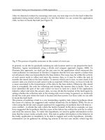
After the AP allocation with the routing (shortest path) is found by the proposed algorithm,
the links in the routing are assigned channels by the algorithm in (Funabiki et al., 2007)
for simulations, whose goal is to find the additional NIC assignment to congested APs for
multiple channels and the channel assignment to the links. The first stage of this two-stage
algorithm repeats one additional NIC assignment to the most congested AP until its given
bound. Then, the second stage sequentially assigns one feasible channel to the link such that
it can minimize the interference between links assigned the same channel. The link channel
assignment is actually realized by assigning the same channel to the NICs at the both end APs
of the link. If some NICs are not assigned any channel, they are moved to different APs and
36
Wireless Mesh Networks
Access-Point Allocation Algorithms for Scalable
Wireless Internet-Access Mesh Networks
9
Fig. 2. AP allocations with three GW positions for network field 1.
the channel assignment is repeated from its first step.
2.5.3 Network field 1
To investigate the optimality of our algorithm in terms of the number of allocated APs and
the maximum hop count, we adopt an artificial symmetric network field that is composed of
16 square rooms with the 60m side as the first field. In each room, 25

(= 5 × 5) host points
are allocated with the 10m interval, and each host point is associated with one host. The 16
host points along the walls in a room are selected as battery points, because electrical outlets
are usually installed on walls. The total of 400 host points are distributed regularly in the
field. The maximum load constraint L is set 25, which indicates that the lower bound on the
number of allocated APs becomes 16 to cover the host points from the calculation of 400
(=
total number o f hosts)/25(= L). For this field, we examine the effect of the GW position for the
AP allocation and the network performance. For this purpose, we prepare three GW positions
as the input to our algorithm, namely in the corner room, in the side room, and in the center room.
Figure 2 illustrates their AP allocations with routings found by our algorithm.
Table 2 summarizes the solution quality indices of our AP allocations for three GW positions
in network field 1. The same single channel is used for every link in network simulations. The
throughput is calculated by dividing the total amount of received packets by the simulation
time. The average result among ten simulation runs using different random numbers for
packet transmissions is used to avoid the bias of random number generations. Our algorithm
finds lower bound solutions in terms of the number of APs (=16 APs) and the maximum hop
count for any GW position. In this field, an AP in any room can communicate with an AP in its
four-neighbor room at the maximum, due to the signal attenuation at the wall. Here, one side
of the room is 60m, and any host point is at least 10 m away from the wall. The communication
range of an AP is reduced to 52m when it passes through one wall, and to 21m when it passes
through two walls. Thus, the minimum hop count to the farthest AP from the GW, which
represents the lower bound on the maximum hop count, is six for the corner room GW, five
for the side room GW, and four for the center room GW. The throughput comparison between
three cases shows that the GW in the center room provides the best one with the smallest hop
count.
37
Access-Point Allocation Algorithms for Scalable Wireless Internet-Access Mesh Networks
10 Wireless Mesh Networks
GW position corner side center

#ofAPs 16 16 16
its lower bound 16 16 16
max. hop count 6 5 4
its lower bound 6 5 4
throughput (Mbps) 12.02 12.08 13.48
Table 2. AP allocation results for network field 1
2.5.4 Simulation results for network field 2
Then, we adopt the second network field that simulates one floor in a building as a more
practical case. This field is composed of two rows of the same rectangular rooms and one
corridor between them. Each row has eight identical rooms with 5m
×10m size. In each room,
15
(= 3 ×5) host points are allocated regularly with one associated host for each point, and the
six host points along the horizontal walls (three along the external wall and three along the
corridor wall) are selected as battery points. Besides, nine battery points are allocated in the
corridor with no host association where the center one is selected as the GW. Thus, the total
number of expected hosts is 240
(= 15 × 16). The maximum load limit L is set 25. As a result,
the lower bound on the number of APs to satisfy the load constraint is 10
(=

240
25

).
Figure 3 shows our AP allocation for this field using 10 APs that are represented by circles.
Every AP other than the GW has a one hop distance from the GW. Thus, our algorithm found
the lower bound solution. For the comparison, a manual allocation using 17 APs is also
depicted there by triangles, where one AP is allocated to each room regularly. The maximum
hop count of this manual allocation is two as shown by lines in the figure.

In network field 2, the effect of the multiple channels for throughputs is investigated by
allocating two NICs (Network Interface Cards) to the GW (Raniwala et al., 2005), in addition to
the single channel case. The channels of links are assigned by using the algorithm in (Funabiki
et al., 2007). Table 3 compares throughputs between two allocations when 1 NIC or 2 NICs
are assigned at the GW. Our allocation provides about 36% better throughput than the manual
allocation for the practical case using the single NIC, by avoiding unnecessary link activations.
Fig. 3. AP allocations for network field 2.
38
Wireless Mesh Networks