Vibration Control Part 2 potx
Bạn đang xem bản rút gọn của tài liệu. Xem và tải ngay bản đầy đủ của tài liệu tại đây (2.85 MB, 25 trang )
Vibration Control
14
mass, the linear approach may seem to be questionable. Nevertheless, the presence of a
mechanical stiffness large enough to overcome the negative stiffness of the electromagnets
makes the linearization point stable, and compels the system to oscillate about it. The
selection of a suitable value of the stiffness k is a trade-off issue deriving from the
application requirements. However, as far as the linearization is concerned, the larger is the
stiffness k relative to
x
k , the more negligible the nonlinear effects become.
2.5.1 Control design
The aim of the present section is to describe the design strategy of the controller that has
been used to introduce active magnetic damping into the system. The control is based on the
Luenberger observer approach (Vischer & Bleuler, 1993), (Mizuno et al., 1996). The adoption
of this approach was motivated by the relatively low level of noise affecting the current
measurement. It consists in estimating in real time the unmeasured states (in our case,
displacement and velocity) from the processing of the measurable states (the current). The
observer is based on the linearized model presented previously, and therefore the higher
frequency modes of the mechanical system have not been taken into account. Afterwards,
the same model is used for the design of the state-feedback controller.
2.5.2 State observer
The observer dynamics is expressed as (Luenberger, 1971):
=XAXBuLyy
•
∧
•∧
⎛⎞
++ −
⎜⎟
⎝⎠
(42)
where X
∧
and y
∧
are the estimations of the system state and output, respectively. Matrix L is
commonly referred to as the gain matrix of the observer. Eq.(42) shows that the inputs of the
observer are the measurement of the current (y) and the control voltage imposed to the
electromagnets (u).
The dynamics of the estimation error ε are obtained combining eq. (39) and eq. (42):
()
= ALC
ε
ε
•
− (43)
where = XX
ε
∧
− . Eq. (43) emphasizes the role of L in the observer convergence. The location
of the eigenvalues of matrix
(
)
ALC− on the complex plane determines the estimation time
constants of the observer: the deeper they are in the left-half part of the complex plane, the
faster will be the observer. It is well known that the observer tuning is a trade-off between
the convergence speed and the noise rejection (Luenberger, 1971). A fast observer is
desirable to increase the frequency bandwidth of the controller action. Nevertheless, this
configuration corresponds to high values of L gains, which would result in the amplification
of the unavoidable measurement noise y, and its transmission into the state estimation. This
issue is especially relevant when switching amplifiers are used. Moreover, the transfer
function that results from a fast observer requires large sampling frequencies, which is not
always compatible with low cost applications.
Electromechanical Dampers for Vibration Control of Structures and Rotors
15
2.5.3 State-feedback controller
A state-feedback control is used to introduce damping into the system. The control voltage
is computed as a linear combination of the states estimated by the observer, with K as the
control gain matrix. Owing to the separation principle, the state-feedback controller is
designed considering the eigenvalues of matrix (A-BK).
Similarly to the observer, a pole placement technique has been used to compute the gains of
K, so as to maintain the mechanical frequency constant. By doing so, the power
consumption for damping is minimized, as the controller does not work against the
mechanical stiffness. The idea of the design was to increase damping by shifting the
complex poles closer to the real axis while keeping constant their distance to the origin
(
12
==
p
pconstant).
2.6 Semi-active transformer damper
Figure 7 shows the sketch of a “transformer” eddy current damper including two
electromagnets. The coils are supplied with a constant voltage and generate the magnetic
field linked to the moving element (anchor). The displacement with speed
q
of the anchor
changes the reluctance of the magnetic circuit and produces a variation of the flux linkage.
According to Faraday’s law, the time variation of the flux generates a back electromotive
force. Eddy currents are thus generated in the coils. The current in the coils is then given by
two contributions: a fixed one due to the voltage supply and a variable one induced by the
back electromotive force. The first contribution generates a force that increases with the
decreasing of the air-gap. It is then responsible of a negative stiffness. The damping force is
generated by the second contribution that acts against the speed of the moving element.
Fig. 7. Sketch of a two electromagnet Semi Active Magnetic Damper (the elastic support is
omitted).
According to eq. (9), considering the two magnetic flux linkages λ
1
and λ
2
of both
counteracting magnetic circuits, the total force acting on the anchor of the system is:
22
21
2
0 air
g
a
p
f
NS
λλ
μ
−
= (44)
The state equation relative to the electric circuit can be derived considering a constant
voltage supply common for both the circuits that drive the derivative of the flux leakage and
the voltage drop on the total resistance of each circuit R=R
coil
+R
add
(coil resistance and
additional resistance used to tune the electrical circuit pole as:
Vibration Control
16
()
()
1
01
2
02
Rg q V
Rg q V
λα λ
λα λ
⋅
⋅
+
−=
+
+=
(45)
Where
0
g
is the nominal airgap and
2
0
2/( )NA
αμ
= .
Eqs.(44) and (45) are linearized for small displacements about the centered position of the
anchor (
0q = ) to understand the system behavior in terms of poles and zero structure
()
()
''
1010
''
2020
,
,
,
qv
R
gq
R
gq
λα λλ
λα λλ
=
=− −
=− +
(46)
(
)
''
02 1
em
F
α
λλ λ
=−. (47)
The term
(
)
00
/VgR
λα
= represents the magnetic flux linkage in the two electromagnets at
steady state in the centered position as obtained from eq.(45) while
1
λ
′
and
2
λ
′
indicate the
variation of the magnetic flux linkages relative to
0
λ
.
The transfer function between the speed
q
and the electromagnetic force F shows a first
order dynamic with the pole (
RL
ω
) due to the R-L nature of the circuits
()
1
1/
em em
RL
FK
qs s
ω
=
+
,
2
2
0
0
2
00
0
2/
,,
2
em RL
RL
NA
VR R
KL
Lg
g
μ
ω
ω
⎛⎞
=− = =
⎜⎟
⎜⎟
⎝⎠
.
(48)
L
0
indicates the inductance of each electromagnet at nominal airgap.
The mechanical impedance is a band limited negative stiffness. This is due to the factor 1/s
and the negative value of
em
K
that is proportional to the electrical power (
mem
KK≥−
)
dissipated at steady state by the electromagnet.
The mechanical impedance and the pole frequency are functions of the voltage supply V
and the resistance R whenever the turns of the windings (N), the air gap area (A) and the
airgap (g
0
) have been defined. The negative stiffness prevents the use of the electromagnet
as support of a mechanical structure unless the excitation voltage is driven by an active
feedback that compensates it. This is the principle at the base of active magnetic
suspensions.
A very simple alternative to the active feedback is to put a mechanical spring in parallel to
the electromagnet. In order to avoid the static instability, the stiffness
m
K of the added
spring has to be larger than the negative electromechanical stiffness of the damper
(
mem
KK≥− ). The mechanical stiffness could be that of the structure in the case of an already
supported structure. Alternatively, if the structure is supported by the dampers themselves,
the springs have to be installed in parallel to them. As a matter of fact, the mechanical spring
in parallel to the transformer damper can be considered as part of the damper.
Electromechanical Dampers for Vibration Control of Structures and Rotors
17
Due to the essential role of that spring, the impedance of eq.(48) is not very helpful in
understanding the behavior of the damper. Instead, a better insight can be obtained by
studying the mechanical impedance of the damper in parallel to the mechanical spring:
()
1/
1
1/ 1/
eq
em em z
m
RL RL
K
FK s
K
vs s s s
ω
ωω
⎛⎞
+
=+=
⎜⎟
⎜⎟
++
⎝⎠
where
e
q
mem
KKK
=
+ ;
e
q
zRL
m
K
K
ωω
= .
(49)
Apart from the pole at null frequency, the impedance shows a zero-pole behavior. To ensure
stability (
0
em m
KK<− < ), the zero frequency (
z
ω
) results to be smaller than the pole
frequency (
0
zRL
ω
ω
<<
).
Figure 8a underlines that it is possible to identify three different frequency ranges:
1.
Equivalent stiffness range (
zRL
ω
ωω
<
<< ): the system behaves as a spring of stiffness
0
eq
K > .
2.
Damping range (
zRL
ω
ωω
<
< ): the system behaves as a viscous damper of coefficient
m
RL
K
C
ω
= (50)
3.
Mechanical stiffness range (
zRL
ω
ωω
<
<< ): the transformer damper contribution
vanishes and the only contribution is that of the mechanical spring (
m
K ) in series to it.
A purely mechanical equivalent of the damper is shown in Figure 8b where a spring of
stiffness
e
q
K is in parallel to the series of a viscous damper of coefficient C and a spring of
stiffness
em
K− . Due to the negative value of the electromagnetic stiffness,
em
K
−
is positive.
It is interesting to note that the resulting model is the same as Maxwell’s model of
viscoelastic materials. At low frequency the system is dominated by the spring
e
q
K while
the lower branch of the parallel connection does not contribute. At high frequency the
viscous damper “locks” and the stiffnesses of the two springs add. The viscous damping
dominates in the intermediate frequency range.
Eq. (50) shows that the product of the damping coefficient C and the pole frequency
RL
ω
is
equal to the mechanical spring stiffness
m
K . A sort of constant gain-bandwidth product
therefore characterizes the damping range of the electromechanical damper. This product is
just a function of the spring stiffness included in the damper. The constant gain-bandwidth
means that for a given electromagnet, an increment of the added resistance leads to a higher
pole frequency (eq. (48)) but reduces the damping coefficient of the same amount. Another
interesting feature of the mechanical impedance of eq. (49) is that the only parameters
affected by the supply voltage V are the equivalent stiffness (K
eq
) and the zero-frequency
(
ω
z
). The damping coefficient (C) and the pole frequency (
RL
ω
) are independent of it.
The substitution of the electromechanical stiffness
em
K of eq. (48) into eq. (49) gives the zero
frequency as function of the excitation voltage
2
2
0
2/
1
zRL
RL m
VR
gK
ωω
ω
⎛⎞
=−
⎜⎟
⎜⎟
⎝⎠
. (51)
Vibration Control
18
Fig. 8. a) mechanical impedance of a transformer eddy current damper in parallel to a spring
of stiffness
m
K . b) Mechanical equivalent.
The larger the supply voltage the smaller the zero frequency and the larger the width of the
damping region. If V=0, there are no electromagnetic forces and the damper reduces to the
mechanical spring. The outcome on the mechanical impedance of a null voltage is that the
zero and the pole frequency become equal. By converse, the largest amplitude of the
damping region is obtained in the limit case when
mem
KK
=
− , i.e. when the mechanical
stiffness is equal to the negative stiffness of the electromagnet. In this case the equivalent
stiffness and therefore the zero frequency are null. As a matter of fact, this last case is of little
or no practical relevance as the system becomes marginally stable.
The equations governing the damping coefficient, the zero and electric pole (eq. (49) - eq.
(51)) outline a design procedure of the damper for a given mechanical structure. Starting
from the specifications, the procedure allows to compute the main parameters of the
damper.
2.6.1 Specifications
The knowledge of (a) the resonant frequencies at which the dampers should be effective and
(b) the maximum acceptable response allows to specify the needed value of the damping
coefficient (C). The pole and zero frequencies (
,
RL z
ω
ω
) have be decided so as the relevant
resonant frequencies fall within the damping range of the damper. Additionally, tolerance
and construction technology considerations impose the nominal airgap thickness g
0
.
Electrical power supply considerations lead to the selection of the excitation voltage V.
2.6.2 Definition of the SAMD parametes
The mechanical stiffness
m
K can be obtained from eq. (50) once the pole frequency (
RL
ω
)
and the damping coefficient (C) are given by the specifications.
The electromechanical parameters of the damper: i.e. the electromechanical constant
2
NA
,
and the total resistance R can be determined as follows:
a.
the required electrical power
2
/VR is obtained from eq. (51). The knowledge of the
available voltage V allows then to determine the resistance R.
b.
The electromechanical constant
2
NA is then found from eq. (48).
3. Experimental results
The present section is devoted to the experimental validation of the models described in
section 2. Two different test benches were used. The former is devoted to validate the
Electromechanical Dampers for Vibration Control of Structures and Rotors
19
models of the motional eddy current dampers while the latter is used to perform
experimental tests on the transformer dampers in active mode (both in sensor and sensorless
configuration), and semi-active mode.
3.1 Experimental validation of the motional eddy current dampers
The aim of the present section is to validate experimentally the model of the eddy current
damper presented in section 2.3; in detail, the experimental work is addressed
•
to confirm that the mechanical impedance ( ()
m
Zs) of a motional eddy current damper
is given by the series of a viscous damper with damping coefficient
em
c
and a linear
spring with stiffness
em
k ,
c.
to validate experimentally that the torque to constant speed characteristic ( ()T Ω ) of a
torsional damper operating as coupler or brake is described by the same parameters
em
c
em
c
and
em
k characterizing the mechanical impedance ( ()
m
Zs).
•
to validate the correlation between the torque to speed characteristic and the
mechanical impedance.
3.1.1 Induction machine used for the experimental tests
A four pole pairs (p = 4) axial flux induction machine has been realized for the steady state
(Figure 9) and vibration tests (Figure 10). The magnetic flux is generated by permanent
magnets while energy is dissipated in a solid conductive disk. The first array of 8 circular
permanent magnets is bond on the iron disk (1) with alternate axial magnetization. The
second array is bond on the disk (2) with the same criterion. Three calibrated pins (9) are
used to face the two iron disk - permanent magnet assemblies ensuring a 1 mm airgap
between the conductor and the magnet arrays. They are circumferentially oriented so that
the magnets with opposite magnetization are faced to each other. In the following such an
assembly is named "stator". The conductor disk (4) is placed in between the two arrays of
magnets and is fixed to the shaft (6). It can rotate relative to the stator by means of two ball
bearings installed in the hub (7 in Figure 10). Table 1 collects the main features of the
induction machine.
Fig. 9. Test rig used for the identification of the motional eddy current machine operating at
steady state. a) View of the test rig. b) Zoom in the induction machine.
Vibration Control
20
Fig. 10. Test rig configured for the vibration tests. a) Front, side view zoomed in the
induction machine. The inpulse hammer force in applied at Point A. b) Lateral view of the
induction machine. c) Top view of the whole test rig.
Feature Unit Value
Number of pole pairs 4
Diameter of the magnets Mm 30
Thickness of the magnets Mm 6
Magnets geometry Circular
Magnets material Nd–Fe–B (N45)
Residual magnetization of the
magnets
T 1.22
Thickness of conductor Mm 7
Conductivity of conductor (Cu) Ω
-1
m
-1
5.7x10
7
Air gap Mm 1
Table 1. Main features of the induction machine used for the tests.
3.1.2 Experimental characterization at steady state
The experimental tests at steady state were carried out to identify the slope c
0
of the torque
to speed characteristic at zero or low speed and the pole frequency
p
ω
. Three type of tests,
defined as "run up", "constant speed" and "quasi - static" have been carried out to this end.
Test rig set up (Figure 9). The electric motor (12 - asynchronous induction motor with rated
power = 2.2 kW ) drives the shaft (6) through the timing belt (16). The conductor disk (4)
rotates with the shaft (6) being rigidly connected to it. The rotation of the stator is
constrained by the bar (11) which connects one of the three pins of the stator to the load cell
fixed to the basement. The tests at steady state are carried out by measuring the torque
generated at different slip speeds
Ω
. The torque is obtained from the measurement of the
tangential force while the slip speed
Ω
is measured using the pick up (13).
Electromechanical Dampers for Vibration Control of Structures and Rotors
21
Run up tests. They are related to a set of speed ramps performed with constant acceleration.
The ramp slopes have been chosen to ensure the steady state condition (a), the minimum
temperature drift (b) and an enough time interval to acquire a significant amount of data (c).
The rated power of the electric motor (12) limits the slip speed to 405 rpm that does not
correspond to the maximum torque velocity (
maxT
Ω
). Nevertheless, the inductive effects
are evidenced allowing the identification of the electric pole
p
ω
(see Figure 11).
Constant Speed Tests. A second set of tests was carried out by measuring the counteracting
torque with the induction machine rotating at a predefined constant slip speed. The aim is to
increase the number of the data at low velocities where the run ups have not supplied
enough points and to confirm the results acquired with the run up procedure.
Fig. 11. Experimental results of the induction machine characterization at steady state.
Fig. 12. Identified values of k
em
in the frequency range 20–80 Hz. Full line, k
em
mean value
obtained as best fit of the experimental points. The experimental points of Z
m
are plotted
with reference to the top-right scale. Full line, Z
m
plotted using c
em
=c
0
and
em em
kk= .
Vibration Control
22
The results of the constant speed tests are plotted in the graph of Figure 11 with circle
marks. Each point represents the average value of a set of 5 tests. The results are consistent
with the expected trend and allow to get more experimental points at low speeds.
Quasi-Static Tests. The aim of the quasi static tests is to characterize the slope c
0
of the torque
to speed curve at very low speed where eq.(28) reduces to
0
=Tc
Ω
(eq. (29)).
A motor driven test is not adequate for an accurate identification of c
0
as the inverter cannot
control the electric motor at rotational speeds lower than 40 rpm The test set up was then
modified locking the rotation of the shaft (6) connected to the conductor disk and enabling
the rotation of the stator assembly. The driving torque was generated by a weight force (mg)
acting tangentially on the stator. This is realized using a ballast (mass m) connected to a
thread wound about the hub (7).
Under the assumption of low constant speed, the slope c
0
can be expressed as
2
0
=
mg t
cr
x
Δ
Δ
(52)
where tΔ indicates the time interval required for the force mg to perform the work
=LmgxΔ while r represents the radius of the hub (m = 0.495 kg, = 1.54x
Δ
m, = 32r mm).
The tests have been carried out by measuring the time interval the ballast needs to cover the
distance xΔ . A set of 5 tests leads to an average slope
0
=1.24c /Nms rad (max deviation
= 5% ). The corresponding torque (
_
=2.67
quasi static
T Nm and speed (
_
= 20.5
quasi static
Ω
rpm)
are reported as the lowest experimental point (asterisk mark
∗
) in the torque to speed curve
of Figure 11. It agrees with the trend of the experimental data obtained at low speed during
the motor driven tests.
Results of the Characterization at Steady State. The electric pole
p
ω
was identified as best fit of
the experimental points reported in the graph of Figure 11 with the model of eq.(28). Being
c
0
already known from the quasi static tests, the identified value of
p
ω
is
0
= 51.1 Hz, ( = 1.24 Nms/rad)
p
c
ω
. (53)
The full line curve plotted in Figure 11 was obtained using the identified values of c
0
and
p
ω
. The good correlation between the identified model and the experimental results can be
considered as a proof of the validity of the steady state model in the investigated speed
range. It derives that the maximum torque and the relative speed that characterize the
induction machine operating at steady state are
0
max max
= = 49.8Nm, = = 766rpm
2
pp
T
c
T
pp
ωω
Ω . (54)
3.1.3 Vibration tests
The aim of the vibration tests is to validate experimentally the mechanical impedance of
eq.(32) using the same induction machine adopted for the constant speed experimental
characterization presented in section 3.1.2.
Test Rig set up. The test rig used for the steady state characterization was modified to realize
a resonant system. The objective is to identify the parameters
em
c and
em
k from the
response at the resonant frequency. To this end the rotation of the conductor disk (4 – Figure
Electromechanical Dampers for Vibration Control of Structures and Rotors
23
10) was constrained by two rigid clamps (14) connected to the basement (a 300 kg seismic
mass). The torsional spring is realized by a cantilever beam acting tangentially on the stator.
Its free end is connected to one of the pins (9) by the axially rigid bar (16) while the
constrained one is clamped by two steel blocks (17) bolted to the basement. The beam
stiffness can be modified by varying its free length. This is obtained by sliding the blocks
(17) relative to it. A set of three beams with different Young modulus and thickness
(aluminum 3 and 5 mm, steel 8 mm) were used to cover the frequency range spanning from
20 Hz to 80 Hz. It's worth to note that the expected pole ω
p
=52 Hz falls in the frequency
range.
Impact tests using an instrumented hammer and two piezoelectric accelerometers were
adopted to measure the frequency response between the tangential force (input) and the
tangential accelerations (outputs), both applied and measured on the stator. Instrumented
hammer and accelerometer signals are acquired and processed by a digital signal analyzer.
Identification Procedure. The identification of the electromechanical model parameters was
carried out by the comparison of the numerical and experimental transfer function
()/ ()Ts s
θ
. The procedure leads to identify the damping coefficient
em
c and the electrical
pole
p
ω
(or the spring stiffness
em
k being = /
p
em em
kc
ω
) of the spring -damper series model
of eq.(32). The value of the electromechanical damping obtained from the steady state
characterization (
0
=1.24c
/Nms rad
) is assumed to be valid also in dynamic vibration
conditions (
0
=
em
cc). Even if this choice blends data coming from the static and the dynamic
tests, it does not compromise the validity of the identification procedure and has been
adopted to reduce the number of unknown parameters. Additionally it allows to perform
the dynamic characterization by means of impact tests only. As a matter of fact, the best
sensitivity for the identification of
em
c could be obtained by setting the resonant frequency
very low compared to the electrical pole (e.g. in the range of
/10
p
ω
). The values of the
static damping, combined with low stiffness required in this case would imply a nearly
critical damping of the resonant mode. This would make the impact test very unsuitable to
excite the system.
The model used for the identification is characterized by a single degree of freedom
torsional vibration system whose inertia is that of the stator ( =J 0.033
2
k
g
m ). The
contribution of the cantilever beam and of the electromagnetic interaction are taken into
account by a mechanical spring with structural damping
(1 )
m
ki
η
+ in parallel to the spring -
viscous damper series of electromagnetic stiffness
em
k and electromagnetic damping
em
c .
The procedure adopted for the identification is the following:
• Impact test without conductor disk to identify the mechanical spring stiffness
m
k and
the related structural damping
η
. This test is repeated for each resonance which is
intended to be investigated.
• Assembly of the conductor disk. This step is carried out without modifying the set up of
the bending spring whose stiffness
m
k
and damping
η
have been identified at the
previous step.
• Impact test with conductor disk.
• Identification of the electromechanical stiffness
em
k that allows the best fit between the
numerical and experimental transfer function.
The procedure is repeated for 23 resonances in the frequency range 20-80 Hz. Figure 13
shows the comparison between the measured FRF and the transfer function of the identified
model in the case of undamped (a) and damped (b) configuration at a resonance of 34 Hz.
Vibration Control
24
Fig. 13. Example of numerical and experimental FRF comparison. a) Identification of the
torsional stiffness k
m
and of the structural damping η b) Identification of k
em
using for c
em
the value obtained by the weight-driven tests (c
em
=1.24 Nms/rad).
The close fit between the model and the experiments indicates that:
• the dynamic model and the relative identification procedure are satisfactory for the
purpose of the present analysis.
• the differential setup adopted for the measurement (accelerations) eliminates the
contribution of the flexural modes from the output response.
• the higher order dynamics (in the range 60 - 120 Hz for the resonance at 34 Hz) are
probably due to a residual coupling that does not affect the identification of k
em
. The
comparison of the experimental curves in Figure 13b) highlights how the not modeled
vibration motion influences the test with and without conductor disk in the same
manner.
Figure 12 shows the results of the identification procedure. The values of the stiffness k
em
, as
identified in each test, are plotted as function of the relevant resonant frequency. Its mean
value is
=399.8 Nm/rad
em
k
(55)
and is plotted as a full line. A standard deviation of 15.24 /Nm rad (3.8% of the mean
value
em
k ) is considered as a proof of the validity of the mechanical impedance model
described by eq.(32). Adopting for
em
c the damping obtained from the weight - driven test
(
0
= = 1.24
em
cc Nms/rad) and for
em
k the values identified by each vibration tests, the
experimental points of Z
m
, as reported in Figure 12, are obtained. The full line in the same
graph refers to eq.(32) in which are adopted for
em
c and
em
k the following parameter:
0
= = 1.24
em
cc Nms/rad and = = 399.8
em em
kk Nm/rad. From that values it follows that the
pole
p
ω
is
Electromechanical Dampers for Vibration Control of Structures and Rotors
25
= / = 51.2 Hz
pemem
kc
ω
(56)
The comparison proves the validity of the models. The small scattering of the experimental
points about the mean value confirm the high predictability of the eddy current dampers
and couplers with the operating conditions.
3.2 Experimental validation of the transformer dampers
Figure 14a shows the test rig used for the experimental characterization of the Transfomer
dampers in active (sensor feedback (AMD) and self-sensing (SSAMD)) and semiactive
(SAMD) configuration. It reproduces a single mechanical degree of freedom. A stiff
aluminium arm is hinged to one end while the other end is connected to the moving part of
the damper. The geometry adopted for the damper is the same of a heteropolar magnetic
bearing. This leads to negligible stray fluxes, and makes the one-dimensional approximation
acceptable for the analysis of the circuit.
The mechanical stiffness required to avoid instability is provided by additional springs. Two
sets of three cylindrical coil springs are used to provide the arm with the required stiffness.
They are preloaded with two screws that allow to adjust the equilibrium position of the arm.
Attention has been paid to limit as much as possible to the friction in the hinge and between
the springs and the base plates. To this end the hinge is realized with two roller bearings
while the contact between the adjustment screws and the base plates is realized by means of
steel balls. Mechanical stops limit to ± 5 degrees the oscillation of the arm relative to the
centred position.
Fig. 14. a) Picture of the test rig b) Test rig scheme.
As shown in Figure 14b, the actuator coils are connected to the power amplifier. If it is
simply a voltage supply, the system works in semi active mode while, when the power
amplifier drives the coils as a current sink, the active configuration is obtained. If the current
value is computed starting from the information of the position sensor, the damper works in
sensor mode, otherwise, if the movement is estimated by using a technique as that described
in section 2.5, the self-sensing operation is obtained.
3.2.1 Active Magnetic Damper (AMD)
When the Transformer damper is configured to operate in AMD mode, the position of the
moving part is measured by means of an eddy current position sensors. Referring to Figure
15 the control system layout is completely decentralized.
Vibration Control
26
Feature Unit Value
Damper- hinge distance mm 320
Spring stiffness N/m 6x30000
Hinge-spring system axis distance mm 160
Magnetic circuit laminations 8 caves/4 electromagnets
Number of turns/electromagnet 142
Nominal air gap mm 0.5
Air gap active area mm
2
420
Coil Resistance Ω 0.4
Additional Resistance Ω 1.0
Coil inductance at nominal air gap mH 10.2
Table 2. Main features of the Transformer damper test bench.
Fig. 15. Scheme of the complete control loop used in the AMD configuration.
The position signal is fed back into the corresponding controller and acts on the collocated
electromagnet. The controller transfer function, capable to provide the required damping
(by a simple PD control loop), is:
8
Re
122 10 1325
383 3 1339
f Current
. (s+.)A
Position (s + . ) (s+ ) m
⋅
⎡
⎤
=
⎢
⎥
⎣
⎦
(57)
The controller output is fed in the power electronic (full H-bridge switching) which current
control loop assures an unitary gain and bandwidth@-3dB of about 1kHz.
The AMD and current loops are implemented on a DSP based electronic board.
The damping performances are evaluated comparing the time response of the closed-loop
with the open-loop system when an impulse excitation is applied to the system. The impulse
excitation is obtained by hitting the system with a hammer. In Figure 16, the open-loop
system response (dashed line) is compared to the closed-loop one when the feedback
controller, reported in eq.(57), is activated.
3.2.2 Self-Sensing Active Magnetic Damper (SSAMD)
The validation of the damper in self-sensing configuration was carried out by implementing
in the DSP based electronic board used for AMD, the observer-controller described in
section 2.5. The current flowing into the coils is measured by means of a hall current sensor
and is fed back into the corresponding obserber-controller. The controller output acts
on the collocated electromagnet. Observer and controllers parameters (poles) are reported in
Table 3.
Electromechanical Dampers for Vibration Control of Structures and Rotors
27
Fig. 16. Time response of the test rig to an impulse excitation. The time response of the
system in two different configurations is plotted as follows: open-loop (dashed line) and
closed-loop based with the AMD controller (solid line).
Poles
p
1
=-3.32+113.35j
p
2
=-3.32-113.35j
Open Loop System
p
2
=-62.6
p
1
=-99.74+113.35j
p
1
=-99.74-113.35j
Observer
(
)
ei
g
ALC−
p
2
=-626.09
p
1
=-29.92+109.38j
p
1
=-29.92-109.38j
State-feedback
controller
(
)
BKAeig
−
p
2
=-500.87
Table 3. Main features of the Transformer damping in different control configuration.
The open-loop voltage-to-displacement transfer function obtained from the model and the
experimental tests are compared in Figure 17a. The correspondence between the two plots is
considered a good validation of the model. The same transfer functions in closed-loop
operation with the controller designed in section 2.5 are compared in Figure 17b. Also in this
case, the correspondence is quite good. This is a proof of the self sensing control strategy
validity. The damping performances are evaluated by analyzing the time response of the
closed-loop system when an impulse excitation is applied to the system.
Fig. 17. Frequency response of the test rig in (a) open-loop and (b) closed-loop configuration
compared to the model. Solid and dashed lines are the model and the plant frequency
responses, respectively.
Vibration Control
28
The impulse excitation is obtained by hitting the system with a hammer. In Figure 18, the
open-loop system response (dashed line) is compared to the closed-loop one when the
observer and state-feedback controller are designed from a model based on the nominal
value of the system parameters. This result is worthy, as it shows that good damping can be
achieved for active magnetic dampers obtained with the simplified model. Furthermore, this
controller does not destabilize the system, as it is the case for full suspension self-sensing
configurations.
Fig. 18. Time response of the test rig to an impulse excitation. The time response of the
system in two different configurations open-loop (dashed line) and closed-loop based on the
identified model (solid line) is plotted.
3.2.3 Semi Active Magnetic Damper (SAMD)
As shown in the Figure 14b, the electrical terminals of each electromagnet are driven by a
voltage power supply and (not shown) are connected in series to an additional resistance.
The value of the additional resistance can be modified to tune the electrical pole frequency.
The natural frequency of the mechanical system can be modified selecting coil spring with
appropriate stiffness. During tests the mechanical frequency was set at 19 Hz and the
electrical pole at 22.3 Hz. The main numerical parameters of the experimental set up are
collected in Table 2.
The validation was performed by comparing the transfer function (FRF) between the input
force and the output acceleration obtained from the experimental tests and that obtained
from the model. The input force was actuated by means of an instrumented hammer; the
acceleration was measured using an accelerometer. The impact point and the accelerometer
are close to the end of the rigid arm. A first series of tests was performed with null excitation
voltage.
The transfer functions obtained from the model are then compared in Figure 19a to the
experimental ones for various excitation voltages.
Solid thick lines in the figure indicate the results from the model while the thin lines refer to
the experimental results. The correlation between the numerical and experimental results
confirms the validity of the adopted modelling approach and of the underlying
assumptions.
As predicted by the model, increasing the voltage supply increases the damping range of
the transformer damper. The modal damping is increased of a factor of about 20 from 0.0073
Electromechanical Dampers for Vibration Control of Structures and Rotors
29
to 0.153 with a power expense of 1.4 W. Even if the damping is increased at the cost of a
reduction of the resonant frequency, the large added damping demonstrates the
effectiveness of the SAMDs. From the point of view of the required power the results
obtained from the single degrees of freedom test bench demonstrates the need of
electromagnets with small airgap and optimised geometry.
The non linear effects are also investigated. The system has been excited with impulse forces
of increasing intensity and leaving constant the voltage supply. Impulse intensities are
chosen so that the amplitude of the oscillation at the beginning of the transient are in a range
0.1-0.6 of the available airgap. The free oscillations due to different initial airgaps are
reported in Figure 19b (voltage supply equal to 0.75 V). Higher displacements are not
allowed due to the attractive force of the electromagnets that makes the system unstable.
Fig. 19. a) Frequency response with various supply voltage for the SAMD b) Time response
with various electromagnets airgaps for the SAMD.
4. Conclusions
The chapter describes the modelling and the experimental validation of different types of
electromagnetic actuators used to damp the vibration in mechanical structures and
machines. The first section describes the theoretical background based on an energetic
approach. Section 2 is devoted to the description and analysis of possible configurations of
electromagnetic actuators. The analysis is supported by the modelling of the different
configurations. In section 3 the experimental validation is presented for four different types
of damping devices: motional eddy current, transformer active based on sensor signal
feedback, transformer active based on self sensing feedback and transformer semi-active.
The analyses described in the present chapter lead to the following results:
-
the vibration response of a motiona eddy current damper can be modeled as the series
connection of a linear mechanical spring and a viscous damper. In general an eddy
current machine behaves as a crank whose end is connected to two spring/damper
series acting along orthogonal directions.
-
The mechanical impedance is a band limited function affected by the pole of the electric
circuit. The band limitation can be usefully exploited in vibration isolation systems
addressed either to reduce the vibration at the fundamental resonant frequency and to
Vibration Control
30
minimize the transmissibility of higher excitation frequency. This feature is of interest
also for eddy current couplers. A proper positioning of the electric pole allows to drive
a load with a continuous torque filtering out the torque irregularities.
-
The parameters describing the behavior of a motional eddy current damper are related
to that of the same device operating at constant speed according to the "conversion
rules" presented section 2.3.
-
The technology of magnetic bearings can be adopted as damping systems if a
mechanical element is introduced to stabilize statically the system. The static stability of
the system allows the adoption of self sensing techniques to feedbach the state of the
structure to be damped. It has been shown that the damping performance of the
Luenberger observer based approach are comparable to the control strategies based on
the position sensor feedback.
-
Electromagnets as that adopted for magnetic bearings can be adopted also as passive or
semi-active damping systems if a constant voltage is supplied to them. In section 1.6 it
was shown that a mechanical impedance of a transformer damper parallel to a
mechanical spring is characterized by a zero and a pole. At frequencies lower than the
zero and higher than the pole, the device behaves as a mechanical spring. Between the
zero and the pole, it operates as a pure viscous damper. The frequency of the pole can
be tuned by adding an external resistance in series to the coil resistance.
5. References
Ahn, Y. K., Yang, B-S. & Morishita S. (2002). Directional Controllable Squeeze Film Damper
Using Electro-Rheological Fluid, ASME Journal of Vibration and Acoustics, Vol. 124,
pp. 105-109.
Crandall, S. H., Karnopp, D., Kurtz, E. F, Pridmore-Brown, E. C. (1968), Dynamics of
Mechanical and Electromechanical Systems, New York: McGraw-Hill.
Genta, G. (2004), Dynamics of Rotating Systems, Springer Verlag.
Genta, G., Festini, A., De Lépine, X. (2008) From oil to magnetic fields: active and passive
vibration control, Acta mechanica et automatica, 2(2), pp. 11-20.
Genta, G., Tonoli, A., Amati, N., Macchi, P., Silvagni, M., and Carabelli, S. (2006), More
electric aeroengines: tradeoff between different electromagnetic dampers and
supports, Tenth International Symposium on Magnetic bearings, EPFL, 21-23 Aug.,
Martigny, Switzerland.
Graves, K. E., Toncich, D., Iovenitti, P. G. (2000), Theoretical Comparison of the Motional
and Transformer EMF Device Damping Efficiency, Journal of Sound and Vibration,
Vol. 233, No. 3, pp 441-453.
Kamerbeek, E. M. H. (1973), Electric motors', Philips tech. Rev., vol. 33, pp. 215 234.
Karnopp, D. (1989), Permanent Magnets Linear Motors used as Variable Mechanical
Damper for Vehicle Suspension, Vehicle System Dynamics, Vol. 18, pp. 1
87-200.
Karnopp, D., Margolis, D. L., Rosenberg, R. C. (1990), System Dynamics: a Unified Approach, J.
Wiley & Sons.
Kligerman, Y. , Gottlieb, O. (1998), Dynamics of a Rotating System with a Nonlinear Eddy-
Current Damper, ASME Journal of Vibration and Acoustics, Vol. 120, pp. 848-853.
Electromechanical Dampers for Vibration Control of Structures and Rotors
31
Kligerman, Y., Grushkevich, A., Darlow, M. S. (1998), Analytical and Experimental
Evaluation of Instability in Rotordynamics System with Electromagnetic
Eddy-Current Damper, ASME Journal of Vibration and Acoustics, Vol. 120, pp. 272-
278.
Luenberger, D. G. (1971), An introduction to observers, IEEE Trans. Autom. Contr, AC-16(6),
pp. 596-602.
Maslen, E., H., Montie, D., T., Iwasaki, T. (2006), Robustness limitations in self-sensing
magnetic bearings, Journal of Dynamic Systems, Measurement and Control, 128, pp.
197-203.
Meisel, J. (1984), Principles of Electromechanical Energy Conversion, Robert Krieger, Malabar,
Florida.
Mizuno, T., Araki, K., Bleuler, H., (1996), Stability analysis of self-sensing magnetic
bearing controllers, IEEE IEEE Transaction of Control System and Technology, 4(5), pp.
572-579.
Mizuno, T., Namiki, H., Araki, K., (1996), Self-sensing operations of frequency-feedback
magnetic bearings, Fifth International Symposium on Magnetic Bearings, 29-30 Aug.,
Kanazawa, Japan, pp. 119-123.
Mizuno, T., Ishii, T., Araki, K. (1998), Self-sensing magnetic suspension using hysteresis
amplifier, Cont. Eng. Pract., 6, pp. 1133-1140.
Nagaya, K. (1984), On a Magnetic Damper Consisting of a Circular Magnetic Flux and a
Conductor of Arbitrary Shape. Part I: Derivation of the Damping Coefficients,
Journal of Dynamic Systems, Measurement and Control, Vol. 106, pp. 46-51.
Nagaya, K. , Karube, Y. (1989), A Rotary Magnetic Damper or Brake Consisting of a Number
of Sector Magnets and a Circular Conductor, Journal of Dynamic Systems,
Measurement and Control, Vol. 111, pp. 97-104.
Noh, M. D., Maslen, E. H. (1997), Self-sensing magnetic bearings using parameter
estimation, IEEE Transaction of Instruments and Measurements, 46(1), pp. 45-50.
Okada, Y., Matsuda, K., Nagai, B. (1992), Sensorless magnetic levitation control by
measuring the PWM carrier frequency component, Third International Symposium on
Magnetic Bearings, 21-31 July, Radisson Hotel, Alexandria, VA.
Schammass, A., Herzog, R., Buhler, P., Bleuler, H. (2005), New results for self-sensing active
magnetic bearings using modulation approach, IEEE Transaction of Control System
and Technology, 13(4), pp. 509-516.
Thibeault, N. M., Smith, R. (2002), Magnetic bearing measurement configurations and
associated robustness and performance limitations, Journal of Dynamic Systems,
Measurement and Control, 124, pp. 589-598.
Tonoli, A., Amati, N., Silvagni, M. (2008), Transformer eddy current dampers for the
vibration control, Journal of Dynamic Systems, Measurement and Control , Vol. 130, pp.
031010-1 - 031010-9.
Vance, J. M. & Ying, D. (2000), Experimental Measurements of Actively Controlled Bearing
Damping with an Electrorheological fluid, ASME Journal of Engineering for Gas
Turbines and Power, Vol. 122, pp 337 - 344.
Vischer, D., and Bleuler, H. (1990), A new approach to sensorless and voltage controlled
AMBs based on network theory concepts, Second International Symposium on
Magnetic bearings, 12-14 July, Tokyo, Japan, pp. 301-306.
Vibration Control
32
Vischer, D., Bleuler, H. (1993), Self-sensing magnetic levitation, IEEE Transaction on
Magnetics, 29(2), pp. 1276-1281.
Tonoli A., Amati N., Bonfitto A., Silvagni M, Staples B., Karpenko E., (2010) - Design of
Electromagnetic Dampers for Aero-Engine Applications, Accepted for Journal of
Engineering for Gas Turbines and Power, ISSN: 0742-4795
2
The Foundation of Electromagnets Based
Active Vibration Control
Ramón Ferreiro García, Manuel Haro Casado* and F. Javier Perez Castelo
University of A Coruña, University of Cadiz*
Spain
1. Introduction
Turbines, pumps, compressors, blowers and all rotating machinery in general, is commonly
used in process industry, including machining tools, power generation, as well as aircraft
and marine propulsion among the most important industrial applications. Mass imbalance
is commonly responsible for rotating machinery vibration. When the principal axis of inertia
of the rotor is not coincident with its geometric axis imbalance occurs. Nevertheless there
are some more causes for rotating machinery vibration such as operation near resonant
frequencies, critical speeds and so on. Higher speeds cause much greater centrifugal
imbalance forces, and the current trend of rotating equipment toward higher power density
clearly leads to higher operational speeds. For instance, speeds approaching 35,000 rpm are
common in machining applications. Therefore, vibration control is essential in improving
machining surface finish; achieving longer bearing, spindle, and tool life in high-speed
machining; and reducing the number of unscheduled shutdowns. A great cost savings for
high-speed turbines, compressors, and other turbomachinery used in petrochemical and
power generation industries can be realized using vibration control technology.
Passive and active vibration control (AVC) techniques of rotating machinery are being used.
It is well established that the vibration of rotating machinery can be reduced by introducing
passive or active devices into the system. Although an active control system is usually more
complicated than a passive vibration control scheme, an AVC technique has many
advantages over a passive vibration control technique.
In (Fuller et al., 1996) it is shown that AVC is more effective than passive vibration control in
general. Furthermore, the passive vibration control is of limited use if several vibration
modes are excited. Finally, because the active actuation device can be adjusted according to
the vibration characteristic during the operation, the active vibration technique is much
more flexible than passive vibration control.
There are two major categories in AVC techniques for rotating machinery:
• Direct active vibration control (DAVC) techniques in which directly apply a lateral
control force to the rotor.
• Active balancing techniques which adjust the mass distribution of a mass redistribution
actuator. Active balancing isn’t under the scope of this chapter.
The control variable in DAVC techniques is a lateral force generated by a force actuator
based on a magnetic bearing. The advantage of DAVC techniques is that the input control
force to the system can be changed according to vibration characteristics.
Vibration Control
34
By applying a fast changing lateral force to the rotating machinery, the total vibration,
including the synchronous vibration, the transient free vibration, and other nonsynchronous
vibration modes of the rotating machinery, can be attenuated or suppressed. The limitation
of most force actuators is the maximum force they can provide. In high rotating speed, the
imbalance-induced force could reach a very high level. As most force actuators cannot
provide sufficient force to compensate for this imbalance-induced force, active balancing
methods are well justified. Although active balancing methods can eliminate imbalance-
induced synchronous vibration, they cannot suppress transient vibration and other
nonsynchronous vibration.
In this chapter DAVC techniques are introduced. Since the mathematical model is the
foundation of any AVC technique, a description of dynamic modelling techniques applied
on rotating machinery is included.
1.1 Dynamic modeling of a planar rotor
The simplest rotor model the planar one. Only the motion in the plane, which is
perpendicular to the rotating shaft, is considered. The geometric setup of the planar rotor
model is shown in figure 1.
Fig. 1. Planar rotor
In this model, the imbalance-induced vibration is described by the particle motion of the
geometric center of the disk. P is the geometric center of the disk, and G is the mass center of
the disk. The motion is represented by the vector r. According to (Childs, 1993) the
governing equation of motion is
2
2
xxx x z
zzz z x
mr cr kr ma ma
mr cr kr ma ma
φ
φ
φ
φ
++= +
++= −
(1)
where m, c, and k are the mass, the viscous damping coefficient, and the shaft-stiffness
coefficient, respectively. [a
X
, a
Z
] is the vector from P to G, expressed in the stationary
coordinate system.
φ
, is the rotating angle of the rotor. For a constant rotating speed,
φ
is
zero. The planar rotor can be used to study the basic phenomena in rotor dynamics such as
critical speed, the effect of damping as well as its associated phenomena.
The planar rotor model is a special case of the model given by (Jeffcott, H. H., 1919), (J.M
Vance, 1987). In the Jeffcott model, the rotor was modelled as a rigid disk supported by a
X
P
Z
φ
r
e
φ
G
P
X
Z
The Foundation of Electromagnets Based Active Vibration Control
35
massless elastic shaft that was mounted on fixed rigid bearings. This model is also
equivalent to a rigid shaft supported by elastic bearings. The major improvement over the
simple planar rotor model is that the motion of the rotor is depicted by rigid body motion
instead of by particle motion. Although this model is a single rigid body model, it ca be
shown the basic phenomena in the motion of the rotor, including the forward and backward
whirling under imbalance force, critical speeds and the gyroscopic effect.
Fig. 2. Rigid Rotor Model
Due to the fact that the natural frequency is a function of the rotating speed, it can also be
predicted by this model. The geometric setup of this model is shown in figure 2.
In this setup, bearings are modelled as isotropic linear spring and damper. The imbalance is
modelled as concentrated mass on the rigid shaft. Two coordinate systems are used: the
body-fixed coordinate oxyz and the inertial coordinate OXYZ. The body-fixed y-axis is the
rotating axis of the shaft, and x and z axes are defined by the other two principal inertia axes
of the rotor. The origin of xyz is selected as the geometric centre of the shaft. The XYZ
coordinate system is the stationary coordinate which is coincident with the xyz coordinate
system under body rest condition. The transverse motion of the rotor is described by the
position of the geometric centre [RX RZ] and by the orientation of the rigid shaft with
respect to the X and Z axes [φ, ψ]. A simplified state space governing equation is shown in
(2) (Zhou & Shi, 2000):
22
22
00001 000
00000 100
00000 010
00000 001
22
00 0 000
22
0 000 00
00 00
22
00 00
12
x
z
x
z
pp
tt tt
pp
tt tt
R
R
kc
mm
d
kc
R
dt
mm
R
II
kL cL
II II
II
kL cL
II II
φφ
φφ
⎡⎤
⎢⎥
⎢⎥
⎡⎤
⎢⎥
⎢⎥
⎢⎥
⎢⎥
⎢⎥
⎢⎥
Θ
⎢⎥
⎢⎥
⎢⎥
−−
Ψ
⎢⎥
⎢⎥
=
⎢⎥
⎢
⎢⎥
−−
⎢
⎢⎥
⎢
⎢⎥
⎢
⎢⎥
Θ
⎢
−−
⎢⎥
⎢
Ψ
⎢⎥
⎣⎦
⎢
⎢
−− −
⎢
⎣⎦
1
2
00
00
00
00
x
z
uz ux
x
ux uz
z
uzy uyz
tt
uyz uxy
tt
R
R
mu mu
f
mm
R
mu mu
f
mm
R
muu muu
II
muu muu
II
⎡⎤
⎢⎥
⎢⎥
⎡⎤
⎢⎥
⎢⎥
⎢⎥
⎢⎥
⎢⎥
⎢⎥
Θ
⎢⎥
−
⎢⎥
⎢⎥
Ψ
⎢⎥
⎡⎤
⎢⎥
+
⎢⎥
⎢⎥
⎥
⎢⎥
⎢⎥
⎣⎦
⎥
⎢⎥
⎢⎥
⎥
⎢⎥
⎢⎥
⎥
⎢⎥
⎢⎥
Θ
⎥
⎢⎥
⎢⎥
⎥
⎢⎥
Ψ
⎢⎥
⎣⎦
⎥
⎢⎥
−
⎥
⎢⎥
⎥
⎢⎥
⎣⎦
(2)
m
u
z
y
Y
Z
u
y
X
x
Vibration Control
36
where L is the length of the shaft; Ip and It are the polar and the diametric moments of
inertia of the shaft, respectively; mu, ux, uy, uz are the mass and the position of the
imbalance in body-fixed coordinate. Exciting forces are defined as:
22
12
cos( ) sin( ), sin( ) cos( )ff
φ
φφ φφφ
=⋅ =⋅
(3)
The model given by (2) can be used on most of the shafts provided that the rigidity of the
shaft is high compared to the supporting bearing. For analysis, simulation and control
objectives the proposed model is considered sufficiently accurate
When flexible rotor models are applied, more complicated rotor system models must be
developed. Such models allows for the elastic deformation of the rotor when in rotation.
Consequently, it is more accurate than the rigid rotor model. A complicated rotor system is
divided into several kinds of basic elements: rigid disk, bearing, flexible shaft segments,
couplings, squeeze-film dampers, and other needed accessories. The equations of motion for
each of these components can be developed using the appropriate force-displacement and
force-velocity relations and the momentum principles as well as other equivalent dynamic
relations. From the above review on rotor dynamics, it is concluded that many powerful
tools for the linear system and frequency response are available. However, most of these
techniques are targeted at the rotor design analysis.
It has been mentioned that for an efficient AVC system synthesis, a suitable analytical model
must be used which is simple in comparison to the overall system equations, while still
providing the essential dynamic characteristics.
(Maslen & Bielk, 1992) presented a stability model for flexible rotors with magnetic bearings.
Besides the flexible rotor model itself, their model included the dynamics of the magnetic
bearing and the sensor-actuator noncollocation. This model can be used for stability analysis
and active vibration synthesis.
Most recently, an analytical imbalance response of the Jeffcott rotor with constant
acceleration was developed by (Zhou & Shi, 2001). They concluded that a satisfactory
solution quantitatively shows that the motion consists of three parts:
•
the transient vibration at damped natural frequency,
•
the synchronous vibration with the frequency of instantaneous rotating speed,
•
and a suddenly occurring vibration at damped natural frequency.
Such mentioned technique provides physical insight into the imbalance-induced vibration
of the rotor during acceleration. For this reason it can be used for the synthesis of AVC
schemes.
For the synthesis of DAVC techniques, most it is common to use simplified low-order finite
element models of the rotor system. Although the techniques developed can be extended to
a high-order system theoretically, the computational load and consequently the signal-to-
noise ratio will have to be higher. The DAVC techniques can be difficult to implement for
the high-order system. Therefore, it is conveniently to use a reduced order models to
approximate the high-order system models. Applied model reduction techniques have a
specific impact on the performance of the DAVC schemes that must be considered if
expected performance cannot be achieved.
1.2 DAVC for rotating machinery
AVC for rotating machinery is considered a special case of AVC for a flexible structure. The
general topic regarding AVC was discussed by (Inman and Simonis, 1987) and (Meirovitch,
The Foundation of Electromagnets Based Active Vibration Control
37
1990). The difference between rotating machinery and other flexible structures is that the
dynamics of the rotor changes with the rotating speed of the shaft. Best control performance
could be achieved if control gains vary with rotating speed. Also, because the shaft is a
moving part, a noncontact actuator is used to apply the control force to the rotating shaft.
There are many types of actuators for direct AVC, including electromagnetic, hydraulic and
piezoelectric as the most important ones. The active magnetic bearing (AMB) is an
established industrial technology with a rapidly growing number of applications. A good
example of the application of magnetic bearings in the machine tool industry can be found
in (Bleuler et al., 1994).
AMB can be used to apply a synchronous force to the shaft to control the imbalance
response, either to cancel the force transmitted to the base or to compensate for the vibration
displacement of the shaft. In (Knospe et al., 1996; Knospe et al., 1995; Knospe, Tamer, &
Fittro, 1997; Knospe, Tamer, & Fedigan, 1997) presented an adaptive open-loop control
method for the imbalance displacement vibration control using AMBs. A synchronous force
that consists of sinusoids that are tied to the shaft angular position via a key phasor signal
was generated and applied to the rotor through the magnetic supporting bearings. The
magnitude and phase of these sinusoids were periodically adjusted so as to minimize the
rotor unbalance response. The magnetic bearings were used to emulate the imbalance-
induced force to offset the force induced by the system imbalance.
Therefore, Knospe and colleagues’ methods are called “active balancing” methods rather
than “DAVC” methods. Other researchers such as (Herzog et al., 1996) and (Lum et al.,
1996) published their work on the imbalance transmitted force controlled by magnetic
bearings.
The basic idea is to use a notch filter to blind the control system of the supporting magnetic
bearing to the imbalance induced response. Therefore, no synchronous forces can be
generated by the magnetic bearings. The rotor will then rotate about its own principal
inertia axis provided that the gap between the shaft and the bearing is large enough. (Fan et
al., 1992) presented a vibration control scheme for an asymmetrical rigid rotor using
magnetic bearings.
Other researchers working in DAVC for rotating machinery adopted a state space
representation of a rotor system. The control inputs are lateral forces. (Balas, 1978) pointed
out that for a feedback control system for flexible systems, the control and observation spill-
over due to the residual (uncontrolled) modes could lead to potential instabilities.
In (Stanway & Burrows, 1981), the dynamic model of the flexible rotor was written in the
state space format and the controllability and observability of the model were studied.
Stanway and Burrows concluded that the lateral motion of the rotor can, under certain
conditions, be stabilized by the application of a single control input to a stationary
component. (Ulsoy, 1984) studied the characteristics of rotating or translating elastic system
vibration problems that are significant for the design of active controllers. The basic
conclusions of his research were that a controller gain matrix that is a function of the
rotating speed is required to maintain a desired closed-loop eigenstructure and that a
residue model spill-over should be handled carefully by the active controller to avoid
instability.
(Firoozian & Stanway, 1988) adopted a full-state observer technique to design a feedback
AVC system.
The stability of the closed-loop system was also studied. To build an AVC system for
flexible structures, the sensor/actuator deployment is an interesting topic. The issue of
Vibration Control
38
actuator/sensor placement for control of flexible structures is an active research area. This
problem is often formulated as a constraint optimization problem. The constraints of this
optimization problem are the limited available locations for the actuators and sensors. The
objective function of this optimization problem is closely related to the control algorithm
used for the flexible structure.
The main possible optimal cost functions for sensor and actuator placement are for system
identification, state estimation (which is represented by the observability) and indirect
control performance (which is represented by the controllability), and direct control
performance (e.g., the transient response, stability).
1.3 Discussion about DAVC
Since rotating machinery is widely used in industry, the AVC of the rotating machinery is
an important engineering problem for both industry and academia. In this introductory
section, a review of the direct vibration control for rotating machinery was conducted.
The major problem faced by the AVC scheme is the use of a limited number of actuators to
control an infinite number of vibration modes. To design an active control scheme, a
reduced-order model should be used and the effect of the spill-over of higher vibration
modes assessed. Although the available techniques developed for dynamic analysis and
active real-time vibration control can be extended to high-order systems theoretically, the
computational load will be heavier and the signal-to-noise ratio of the vibration
measurement will have to be higher. Hence, the available techniques could be difficult to
implement in high-order systems. Consequently, it is necessary to use a model reduced
system to approximate the high-order system.
In most of AVC methods, the imbalance estimation is coupled with the control strategy. So
far, there are no systematic methods available to show the relationship between the
estimation and the control strategy. A control action is preferable if it can obtain small
imbalance-induced vibration and excite the system to obtain the good imbalance estimation
at the same time.
Thus, coupling effects should be investigated by considering the estimation algorithm, the
system dynamics, and the control performance. This research can also lay a scientific
foundation for the design of an efficient and reliable generic adaptive control system.
It is clear that the active balancing can improve product quality and improve the fatigue life
of the machine and cutting tools and, hence, reduce the system cost. However, the
installation and maintenance of an active vibration system for rotating machinery will
increase the system cost. How to assess the AVC system from a cost-effective point of view
and on a higher process level is not well studied in the literature. More that two decades of
experience demonstrates that this is an interesting and important problem in the AVC of
rotating machinery.
2. AVC with magnetic actuators
2.1 Introduction
Unbalance response is a common vibration problem associated with rotating machinery.
During several years, researchers have demonstrated that this vibration could be greatly
alleviated for machines using active magnetic bearings through active magnetic control.
Many of the control strategies employed fall into a class which the authors have termed
adaptive open loop control.