Design for Six Sigma (DfSS) in Software 133

4.2 Software FMEA
Failure mode and effects analysis (FMEA) is one of the well-known analysis methods having
an established position in the traditional reliability analysis. The purpose of FMEA is to
identify “UPFRONT” possible failure modes of the system components, evaluate their
influences on system behaviour and propose proper countermeasures to suppress these
effects. A failure mode and effects analysis (FMEA) can be described as a systematic way of
identifying failure modes of a system, item or function, and evaluating the effects of the
failure modes on the higher level. A bottom-up technique such as FMEA is an effective way
to identify component failures or system mal-functions, and to “design rightly” the system
under consideration (Pentti & Atte, 2002).
The standard guidelines provided by the FMEA cannot be directly used and would have to
be tailored for applying it to software. Typically the best definition for “Severity” would be
the one that the software teams use for their problem report classifications. Similarly for
“Occurrence” and “Detection” it is better that the teams use their own tailored guideline
based on a simplistic criteria of “Very high” to “Very Low”.
By nature, software failure modes generally are unknown—“software modules do not fail in
the literal sense as hardware failure, they only display incorrect behaviour”—and depend
on dynamic behaviour of the application. The aim of the FMEA is to then uncover those
situations.

The following are certain alerts/pitfalls/learning’s to be aware of when doing software
FMEA:-
1) Use case explosion – Software due to its very nature has many permutations
/combinations of inputs and outputs which could be prone to failures. Hence FMEA
would soon run into thousands of use-case combinations of failure-modes. Hence it is
advisable to focus on failure modes associated with CTQs, Critical
components/modules/functionalities etc
2) Capturing “Requirements not meeting” as failure modes e.g. set not recording as a
failure mode for a DVD recorder etc. Recording is a basic requirement itself of a

recorder so listing it as failure mode at a global level would not help. Instead the failure
mode should delve deeper into the features
3) Not having the appropriate subject matter experts in the analyses. Failure modes
largely dependent on competence, hence knowledge of domain (not software
engineering but rather the usage of product in actual environment) is crucial
4) Attempting to perform FMEA on 100% of the design or code instead of sampling the
design/code most likely to cause a serious failure
5) Excluding hardware from the analysis or isolating the software from the rest of the
system as many of the failures result from the combination and not software alone
6) Typically for software, the severity “SEV” would remain unchanged and it is mainly
the occurrence and detection that can be improved. For e.g. a hang/crash in a normal
user operation is a severity “A” failure mode translating to a value of 8 for SEV. By
taking various actions, its occurrence can be reduced/ eliminated or detectability can be
improved. However even after taking actions, the severity would remain unchanged
7) The occurrence “OCC” value can be tricky sometimes for software. In a product
development environment, normally a test will be done on few devices say 5 to 10 and
issues do not surface out. When long duration tests are conducted in the factory on a

larger sample say 100 devices then the product starts failing. So OCC value could be
different based on the sample taken and has to be accordingly adapted when validating
the results
8) From software development life-cycle perspective, the DET value can take on different
values for the same detection levels. For e.g. a control mechanism may have a high
chance of detecting a failure mode making the DET value 4 as per the guideline.
However based on whether that detection can happen in design itself or testing may
vary the value. The team might give a higher vale for DET for something that can be
detected only in testing as against that which can be detected in design.

4.3 Use of Statistics in software
Often this is one of most important challenge when it comes to using concepts like DfSS for

software. Many software requirements fall into the Yes/No, Pass/Fail category so limit
setting is fuzzy. Most of them would become critical factors (CFs) and not CTQs in the
“continuous data” sense
 Predicting DPMO (defects per million opportunities) may be misleading (out of limits).
This is because the specifications limits in cases like responsiveness are soft targets. Just
because it takes 0.5 seconds more than Upper Specification Limit to start-up does not
necessarily classify it as a defective product. In Six sigma terms anything beyond Upper
spec limit and less than Lower spec limit becomes a defect
 Random failures due to only software are rare due to which concept like Mean-Time-
Between-Failures (MTBF) for software alone is questionable, however it makes sense at
overall product level
 No concept of samples – the same piece of code is corrected and used, so advanced
statistical concepts have to be applied with discretion

However this does not mean that statistical concepts cannot be applied at all.

 The starting point is to challenge each specification to ensure if some numbers can be
associated with it. Even abstract elements such as “Usability” can be measured as seen
in section 3.5.2
 For many of the software CTQs, the Upper limits and lower limits may not be hard
targets, nevertheless it is a good to use them as such and relax it during the course of
the development
 The change in Z-scores over the releases would be more meaningful rather than
absolute Z-scores
 All Statistical concepts can be applied for the “Continuous CTQs”
 Many of the Design of experiments in software would happen with discrete Xs due to
nature of software. So often the purpose of doing these is not with the intent of
generating a transfer function but more with a need to understand which “Xs” impact
the Y the most – the cause and effect. So the Main effects plot and Interaction plots have
high utility in such scenarios

 The hypothesis tests such as t-Tests, F-Tests, ANOVA are useful in the Verify and
Monitor phase to determine if indeed there have been statistical significant changes
over the life cycle or from one product generation to next etc.
Quality Management and Six Sigma134

 Statistical Capability analysis to understand the variation on many of the CTQs in
simulated environments as well as actual hardware can be a good starting point to
design in robustness in the software system.

5. References
Ajit Ashok Shenvi (2008). Design for Six Sigma : Software Product Quality, Proceedings of the
1st India Software Engineering Conference, pp. 97-106, ISBN:978-1-59593-917-3,
Hyderabad, India, February 19 - 22, 2008. ISEC '08. ACM, New York, NY, DOI=
/>
Haapanen Pentti & Helminen Atte, Stuk-yto-tr 190/August 2002. Failure modes and effects
analysis of software based-automation systems
Jeannine M. Siviy and Eileen C. Forrester. (2004). Accelerating CMMi adoption using Six
Sigma,Carnegie Mellon Software Engineering Institute
Jeannine M. Siviy (SEI), Dave Halowell (Six Sigma advantage). 2005. Bridging the gap
between CMMi & Six Sigma Training. Carnegie Mellon Sw Engineering Institute
Jiantao Pan. 1999. Software Reliability. Carnegie Mellon
/>
Minitab tool – Statistical tool.

Philips DFSS training material for Philips. 2005. SigMax Solutions LLC, USA
Statistical Process Control for Software: Fill the Gap 135
Statistical Process Control for Software: Fill the Gap
Maria Teresa Baldassarre, Nicola Boffoli and Danilo Caivano
X


Statistical Process Control
for Software: Fill the Gap

Maria Teresa Baldassarre, Nicola Boffoli and Danilo Caivano
University of Bari
Italy

1. Introduction
The characteristic of software processes, unlike manufacturing ones, is that they have a very
high human-centered component and are primarily based on cognitive activities. As so, each
time a software process is executed, inputs and outputs may vary, as well as the process
performances. This phenomena is better identified in literature with the terminology of
“Process Diversity” (IEEE, 2000). Given the characteristics of a software process, its intrinsic
diversity implies the difficulty to predict, monitor and improve it, unlike what happens in
other contexts. In spite of the previous observations, Software Process Improvement (SPI) is a
very important activity that cannot be neglected. To face these problems, the software
engineering community stresses the use of measurement based approaches such as QIP/GQM
(Basili et al., 1994) and time series analysis: the first approach is usually used to determine
what improvement is needed; the time series analysis is adopted to monitor process
performances. As so, it supports decision making in terms of when the process should be
improved, and provides a manner to verify the effectiveness of the improvement itself.
A technique for time series analysis, well-established in literature, which has given
insightful results in the manufacturing contexts, although not yet in software process ones is
known as Statistical Process Control (SPC) (Shewhart, 1980; Shewhart, 1986). The technique
was originally developed by Shewhart in the 1920s and then used in many other contexts.
The basic idea it relies on consists in the use of so called “control charts” together with their
indicators, called run tests, to: establish operational limits for acceptable process variation;
monitor and evaluate process performances evolution in time. In general, process
performance variations are mainly due to two types of causes classified as follows:
 Common cause variations: the result of normal interactions of people, machines,

environment, techniques used and so on.
 Assignable cause variations: arise from events that are not part of the process and
make it unstable.
In this sense, the statistically based approach, SPC, helps determine if a process is stable or
not by discriminating between common cause variation and assignable cause variation. We
can classify a process as “stable” or “under control” if only common causes occur. More
precisely, in SPC data points representing measures of process performances are collected.
8
Quality Management and Six Sigma136

These values are then compared to the values of central tendency, upper and lower limit of
admissible performance variations.
While SPC is a well established technique in manufacturing contexts, there are only few
works in literature (Card, 1994; Florac et al., 2000; Weller, 2000(a); Weller, 2000(b); Florence,
2001; Sargut & Demirors, 2006; Weller, & Card. 2008; Raczynski & Curtis, 2008) that present
successful outcomes of SPC adoption to software. In each case, not only are there few cases
of successful applications but they don’t clearly illustrate the meaning of control charts and
related indicators in the context of software process application.
Given the above considerations, the aim of this work is to generalize and put together the
experiences collected by the authors in previous studies on the use of Statistical Process
Control in the software context (Baldassarre et al, 2004; Baldassarre et al, 2005; Caivano 2005;
Boffoli, 2006; Baldassarre et al, 2008; Baldassarre et al, 2009) and present the resulting
stepwise approach that: starting from stability tests, known in literature, selects the most
suitable ones for software processes (tests set), reinterprets them from a software process
perspective (tests interpretation) and suggest a recalculation strategy for tuning the SPC
control limits.
The paper is organized as follows: section 2 briefly presents SPC concepts and its
peculiarities; section 3 discusses the main differences and lacks of SPC for software and
presents the approach proposed by the authors; finally, in section 4 conclusions are drawn.


2. Statistical Process Control: Pills
Statistical Process Control (SPC) (Shewhart, 1980; Shewhart, 1986) is a technique for time
series analysis. It was developed by Shewhart in the 1920s and then used in many contexts.
It uses several “control charts” together with their indicators to establish operational limits
for acceptable process variation. By using few data points, it is able to dynamically
determine an upper and lower control limit of acceptable process performance variability.
Such peculiarity makes SPC a suitable instrument to detect process performance variations.
Process performance variations are mainly due to: common cause variations (the result of
normal interactions of people, machines, environment, techniques used and so on);
assignable cause variations (arise from events that are not part of the process and make it
unstable). A process can be described by measurable characteristics that vary in time due to
common or assignable cause variations. If the variation in process performances is only due
to common causes, the process is said to be stable and its behavior is predictable within a
certain error range; otherwise an assignable cause (external to the process) is assumed to be
present and the process is considered unstable. A control chart usually adopts an indicator
of the process performances central tendency (CL), an upper control limit (UCL =
CL+3sigma) and a lower control limit (LCL = CL-3sigma). Process performances are tracked
overtime on a control chart, and if one or more of the values fall outside these limits, or
exhibit a “non random” behavior, an assignable cause is assumed to be present.


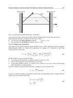
Fig. 1. Example of SPC charts (X charts)

“Sigma” is calculated by using a set of factors tabulated by statisticians (for more details
refer to (Wheeler & Chambers, 1992)) and it is based on statistical reasoning, simulations
carried out and upon the heuristic experience that: “it works”. A good theoretical model for
a control chart is the normal distribution shown in figure 2 where: the percentage values
reported express the percentage of observations that fall in the corresponding area;  is the
theoretical mean;  is the theoretical standard deviation. In the [-3, +3] interval, fall
99.73% (i.e. 2.14 + 13.59 + 34.13 + 34.13 + 13.59 + 2.14) of the total observations. Thus only

the 0,27 % of the observations is admissible to fall outside the [-3, +3] interval.

Fig. 2. Normal distribution, the bell curve

If we consider sigma in place of , the meaning and rational behind a control chart results
clear. For completeness it is necessary to say that the normal distribution is only a good
theoretical model but, simulations carried out have shown that independently from the data
distribution, the following rules of thumb work:
 Rule1: from 60% to 75% of the observations fall in the [CL-sigma, CL+1sigma]
 Rule2: from 90% to 98% of the observations fall in the [CL-2sigma, CL+2sigma]
 Rule3: from 99% to 100% of the observations fall in the [CL-3sigma, CL+3sigma]
Statistical Process Control for Software: Fill the Gap 137

These values are then compared to the values of central tendency, upper and lower limit of
admissible performance variations.
While SPC is a well established technique in manufacturing contexts, there are only few
works in literature (Card, 1994; Florac et al., 2000; Weller, 2000(a); Weller, 2000(b); Florence,
2001; Sargut & Demirors, 2006; Weller, & Card. 2008; Raczynski & Curtis, 2008) that present
successful outcomes of SPC adoption to software. In each case, not only are there few cases
of successful applications but they don’t clearly illustrate the meaning of control charts and
related indicators in the context of software process application.
Given the above considerations, the aim of this work is to generalize and put together the
experiences collected by the authors in previous studies on the use of Statistical Process
Control in the software context (Baldassarre et al, 2004; Baldassarre et al, 2005; Caivano 2005;
Boffoli, 2006; Baldassarre et al, 2008; Baldassarre et al, 2009) and present the resulting
stepwise approach that: starting from stability tests, known in literature, selects the most
suitable ones for software processes (tests set), reinterprets them from a software process
perspective (tests interpretation) and suggest a recalculation strategy for tuning the SPC
control limits.
The paper is organized as follows: section 2 briefly presents SPC concepts and its

peculiarities; section 3 discusses the main differences and lacks of SPC for software and
presents the approach proposed by the authors; finally, in section 4 conclusions are drawn.

2. Statistical Process Control: Pills
Statistical Process Control (SPC) (Shewhart, 1980; Shewhart, 1986) is a technique for time
series analysis. It was developed by Shewhart in the 1920s and then used in many contexts.
It uses several “control charts” together with their indicators to establish operational limits
for acceptable process variation. By using few data points, it is able to dynamically
determine an upper and lower control limit of acceptable process performance variability.
Such peculiarity makes SPC a suitable instrument to detect process performance variations.
Process performance variations are mainly due to: common cause variations (the result of
normal interactions of people, machines, environment, techniques used and so on);
assignable cause variations (arise from events that are not part of the process and make it
unstable). A process can be described by measurable characteristics that vary in time due to
common or assignable cause variations. If the variation in process performances is only due
to common causes, the process is said to be stable and its behavior is predictable within a
certain error range; otherwise an assignable cause (external to the process) is assumed to be
present and the process is considered unstable. A control chart usually adopts an indicator
of the process performances central tendency (CL), an upper control limit (UCL =
CL+3sigma) and a lower control limit (LCL = CL-3sigma). Process performances are tracked
overtime on a control chart, and if one or more of the values fall outside these limits, or
exhibit a “non random” behavior, an assignable cause is assumed to be present.


Fig. 1. Example of SPC charts (X charts)

“Sigma” is calculated by using a set of factors tabulated by statisticians (for more details
refer to (Wheeler & Chambers, 1992)) and it is based on statistical reasoning, simulations
carried out and upon the heuristic experience that: “it works”. A good theoretical model for
a control chart is the normal distribution shown in figure 2 where: the percentage values

reported express the percentage of observations that fall in the corresponding area;  is the
theoretical mean;  is the theoretical standard deviation. In the [-3, +3] interval, fall
99.73% (i.e. 2.14 + 13.59 + 34.13 + 34.13 + 13.59 + 2.14) of the total observations. Thus only
the 0,27 % of the observations is admissible to fall outside the [-3, +3] interval.

Fig. 2. Normal distribution, the bell curve

If we consider sigma in place of , the meaning and rational behind a control chart results
clear. For completeness it is necessary to say that the normal distribution is only a good
theoretical model but, simulations carried out have shown that independently from the data
distribution, the following rules of thumb work:
 Rule1: from 60% to 75% of the observations fall in the [CL-sigma, CL+1sigma]
 Rule2: from 90% to 98% of the observations fall in the [CL-2sigma, CL+2sigma]
 Rule3: from 99% to 100% of the observations fall in the [CL-3sigma, CL+3sigma]
Quality Management and Six Sigma138

The control limits carried out using SPC are based on a process observation and they are
expression of it. They are not the result of expert judgment and, furthermore, they can be
clearly obtained.
In general, control charts are used as follows: samples are taken from the process, statistics
(for example, average and range) are calculated and plotted on charts, and the results are
interpreted with respect to process limits or, as they are known in SPC terminology, control
limits. Control limits are the limits within which the process operates under normal
conditions. They tell us how far we can expect sample values to stray from the average
given the inherent variability of the process or, to use the SPC terms, the magnitude of
common-cause variation. Data points beyond the control limits or other unusual patterns
indicate a special-cause variation.

3. SPC for Software
Software processes and manufacturing ones present deep differences that the use of SPC in

software cannot exempt from considering. Moreover, according to the discussions in (Jalote,
2002(a); Eickelmann & Anant, 2003) we can consider three main differences between
manufacturing and software processes that have to be kept in mind in order to assure a
more appropriate use of SPC in software context in terms of control charts, run test
indicators, anomalies interpretation and control limits calculation.

Measurement of Software Processes. In manufacturing, the observed and actual number of
defects is not significantly different. In software development, these two numbers routinely
vary significantly. Possible causes for extreme variation in software measurement include
the following:
 People are the software production process.
 Software measurement might introduce more variation than the process itself.
 Size metrics do not count discrete and identical units.
Such extreme variations in software processes need different indicators for the anomalies
detection and more specific interpretations.

Product Control and Product Rework. The primary focus of using SPC control charts in
manufacturing is to bring the process back in control by removing assignable causes and
minimize as much as possible the future production losses. In the manufacturing process
when an anomaly occurs the products usually do not conform to the expected standards
and therefore, must be discarded. On the other hand, in the software process the product
can be “reworked”. For example, when using control charts for an inspection process, if a
point falls outside the control limits, besides the process improvement actions like
improving the checklist, inevitably, product improvement actions like re-reviews,
scheduling extra testing also occurs. With software processes, besides improving the
process, an important objective of using control charts is to also control the product. In
(Gardiner & Montgomery, 1987), which is perhaps the first paper on the use of SPC in
software, Gardiner and Montgomery suggest "rework" as one of the three actions that
management should carry out if a point falls outside the control limits. The use described in
(Ebenau, 1994) clearly shows this aspect of product control. The survey of high maturity

organizations also indicates that project managers also use control charts for project-level

control (Jalote, 2002(b)). Due to this product-control, project managers are more likely to
want test indicators and interpretations that highlight potential warning signals, rather than
risk to miss such signals, even if it means more false alarms.

Shutdown and Startup is “Cheaper”. The cost parameters that affect the selection of control
limits are likely to be quite different in software processes. For example, if a manufacturing
process has to be stopped (perhaps because a point falls outside the control limits), the cost
of doing so can be quite high. In software, on the other hand, the cost of stopping a process
is minimal as elaborate "shutdown" and "startup" activities are not needed. Similarly, the
cost of evaluating a point that falls outside the control limits is likely to be very different in
software processes as compared to manufacturing ones. For these reasons the control limits
could be recalculated more often than in manufacturing processes.
Due to these differences, it is reasonable to assume that, to get the best results, control
charts, the use of the indicators and their interpretation, as well as the tuning of process
limits, will need to be adapted to take into account the characteristics of software processes.

Finally, in spite of the rather simple concepts underlying statistical process control, it is
rarely straightforward to implement (Card, 1994). The main lacks for software processes are
listed below:

Focus on individual or small events. The indicators generally used in SPC highlight
assignable causes related to the individual events. However the high variability of a
software process and its predominant human factor make such indicators ineffective
because they usually discover occasional variations due to passing phenomena that should
be managed as false positives (false alarms).
Therefore the SPC indicators, in software processes, should detect the assignable variations
and then also interpret them if occasional variations (as false positives) or occurred changes
in the process (in the manufacturing processes the passing phenomena are very rare). For

such reasons the control charts should be constructed with a view toward detecting process
trends rather than identifying individual nonconforming events (Figure 3).


Fig. 3. SPC variations tree
Statistical Process Control for Software: Fill the Gap 139

The control limits carried out using SPC are based on a process observation and they are
expression of it. They are not the result of expert judgment and, furthermore, they can be
clearly obtained.
In general, control charts are used as follows: samples are taken from the process, statistics
(for example, average and range) are calculated and plotted on charts, and the results are
interpreted with respect to process limits or, as they are known in SPC terminology, control
limits. Control limits are the limits within which the process operates under normal
conditions. They tell us how far we can expect sample values to stray from the average
given the inherent variability of the process or, to use the SPC terms, the magnitude of
common-cause variation. Data points beyond the control limits or other unusual patterns
indicate a special-cause variation.

3. SPC for Software
Software processes and manufacturing ones present deep differences that the use of SPC in
software cannot exempt from considering. Moreover, according to the discussions in (Jalote,
2002(a); Eickelmann & Anant, 2003) we can consider three main differences between
manufacturing and software processes that have to be kept in mind in order to assure a
more appropriate use of SPC in software context in terms of control charts, run test
indicators, anomalies interpretation and control limits calculation.

Measurement of Software Processes. In manufacturing, the observed and actual number of
defects is not significantly different. In software development, these two numbers routinely
vary significantly. Possible causes for extreme variation in software measurement include

the following:
 People are the software production process.
 Software measurement might introduce more variation than the process itself.
 Size metrics do not count discrete and identical units.
Such extreme variations in software processes need different indicators for the anomalies
detection and more specific interpretations.

Product Control and Product Rework. The primary focus of using SPC control charts in
manufacturing is to bring the process back in control by removing assignable causes and
minimize as much as possible the future production losses. In the manufacturing process
when an anomaly occurs the products usually do not conform to the expected standards
and therefore, must be discarded. On the other hand, in the software process the product
can be “reworked”. For example, when using control charts for an inspection process, if a
point falls outside the control limits, besides the process improvement actions like
improving the checklist, inevitably, product improvement actions like re-reviews,
scheduling extra testing also occurs. With software processes, besides improving the
process, an important objective of using control charts is to also control the product. In
(Gardiner & Montgomery, 1987), which is perhaps the first paper on the use of SPC in
software, Gardiner and Montgomery suggest "rework" as one of the three actions that
management should carry out if a point falls outside the control limits. The use described in
(Ebenau, 1994) clearly shows this aspect of product control. The survey of high maturity
organizations also indicates that project managers also use control charts for project-level

control (Jalote, 2002(b)). Due to this product-control, project managers are more likely to
want test indicators and interpretations that highlight potential warning signals, rather than
risk to miss such signals, even if it means more false alarms.

Shutdown and Startup is “Cheaper”. The cost parameters that affect the selection of control
limits are likely to be quite different in software processes. For example, if a manufacturing
process has to be stopped (perhaps because a point falls outside the control limits), the cost

of doing so can be quite high. In software, on the other hand, the cost of stopping a process
is minimal as elaborate "shutdown" and "startup" activities are not needed. Similarly, the
cost of evaluating a point that falls outside the control limits is likely to be very different in
software processes as compared to manufacturing ones. For these reasons the control limits
could be recalculated more often than in manufacturing processes.
Due to these differences, it is reasonable to assume that, to get the best results, control
charts, the use of the indicators and their interpretation, as well as the tuning of process
limits, will need to be adapted to take into account the characteristics of software processes.

Finally, in spite of the rather simple concepts underlying statistical process control, it is
rarely straightforward to implement (Card, 1994). The main lacks for software processes are
listed below:

Focus on individual or small events. The indicators generally used in SPC highlight
assignable causes related to the individual events. However the high variability of a
software process and its predominant human factor make such indicators ineffective
because they usually discover occasional variations due to passing phenomena that should
be managed as false positives (false alarms).
Therefore the SPC indicators, in software processes, should detect the assignable variations
and then also interpret them if occasional variations (as false positives) or occurred changes
in the process (in the manufacturing processes the passing phenomena are very rare). For
such reasons the control charts should be constructed with a view toward detecting process
trends rather than identifying individual nonconforming events (Figure 3).


Fig. 3. SPC variations tree
Quality Management and Six Sigma140

Failure to investigate and act. Statistical process control only signals that a problem may
exist. If you don’t follow through with a detailed investigation, like an audit, and follow-up

corrective action, there is no benefit in using it. In these sense a larger set of anomalies
indicators and a more precise anomalies interpretation is necessary.

Incorrect computation of control limits. Several formulas exist for computing control limits
and analyzing distributions in different situations. But although they are straightforward,
without proper background, it is easy to make mistakes. Such mistakes might concern:
 the correct calculation of control limits
 the appropriate timing for the recalculation of control limits (“tuning” activities)

In order to mitigate such differences and face these issues, in the past the authors have
proposed and experimented an SPC framework for software processes (Baldassarre et al.,
2007). Such framework, based on the software process peculiarities, proposes the most
appropriate control charts, a set of indicators (run-test set) and related interpretations (run-
test interpretation) in order to effectively monitor process variability. When such indicators
are used, SPC is able to discover software process variations and discriminate between
them. For these reasons such indicators:
 are able to detect process trends rather than identify individual nonconforming
events (i.e. occasional variations that in software processes would be considered like
the false alarms)
 enable to discover assignable variations and address some quality information about
“what happens” in the process. Thereby such framework supports the manager
during the causes-investigation activities.
Furthermore, our framework faces problems related to incorrect computation of control
limits and proposes “when” and “how” to recalculate the SPC control limits (the “tuning”
activities) that supports manager in:
 Choosing the control charts and measurement object to use in SPC analysis
 Selecting the appropriate data-points, building the Reference Set and calculating
the control limits needed for monitoring process variations
 Monitoring the process variations and detecting run-tests failures
 Evaluating the assignable events occurred and then undertaking the appropriate

actions (for example recalculating the control limits)
Figure 4 summarizes the steps for applying the framework: first, process characterization is
carried out, i.e. a process characteristic to monitor is observed over time, and related data
points are collected; the appropriate control chart is selected and upper and lower control
limits are calculated (Step 1); secondly anomaly detection occurs, i.e. each new data point
observed is plotted on the chart, keeping control limits and central line the same; the set of
run tests (RT1…RT8) is executed and anomalies are detected each time a test fails (Step 2); at
this point, causes investigation is carried out, i.e. the cause of the anomaly pointed out is
investigated in order to provide an interpretation (Step 3). Finally, according to the process
changes occurred and identified in the previous step, appropriate tuning actions are applied
to tune the sensibility of the monitoring activity and adapt it to the new process
performances (Step 4).



Fig. 4. SPC based Process Monitoring guidelines

3.1 Process Characterization
A reference set must be determined in order to characterize a process, i.e. a set of
observations that represent the process performances and do not suffer from exceptional
causes. In short, the reference set provides a reference point to compare the future
performances with. After determining the reference set, each following observation must be
traced on the control chart obtained and then the set of tests included in the test set must be
carried out in order to identify if eventual exceptional causes come up. More precisely, the
following two steps are executed:
• Identify the measurement object
• Identify the reference set

Identify the measurement object. The process to evaluate is identified along with the
measurement characteristics that describe the performances of interest. The most

appropriate control charts for the phenomena being observed are selected. There are charts
for variables data (measurement data such as length, width, thickness, and moisture
content) and charts for attributes data (“counts” data such as number of defective units in a
sample).

Statistical Process Control for Software: Fill the Gap 141

Failure to investigate and act. Statistical process control only signals that a problem may
exist. If you don’t follow through with a detailed investigation, like an audit, and follow-up
corrective action, there is no benefit in using it. In these sense a larger set of anomalies
indicators and a more precise anomalies interpretation is necessary.

Incorrect computation of control limits. Several formulas exist for computing control limits
and analyzing distributions in different situations. But although they are straightforward,
without proper background, it is easy to make mistakes. Such mistakes might concern:
 the correct calculation of control limits
 the appropriate timing for the recalculation of control limits (“tuning” activities)

In order to mitigate such differences and face these issues, in the past the authors have
proposed and experimented an SPC framework for software processes (Baldassarre et al.,
2007). Such framework, based on the software process peculiarities, proposes the most
appropriate control charts, a set of indicators (run-test set) and related interpretations (run-
test interpretation) in order to effectively monitor process variability. When such indicators
are used, SPC is able to discover software process variations and discriminate between
them. For these reasons such indicators:
 are able to detect process trends rather than identify individual nonconforming
events (i.e. occasional variations that in software processes would be considered like
the false alarms)
 enable to discover assignable variations and address some quality information about
“what happens” in the process. Thereby such framework supports the manager

during the causes-investigation activities.
Furthermore, our framework faces problems related to incorrect computation of control
limits and proposes “when” and “how” to recalculate the SPC control limits (the “tuning”
activities) that supports manager in:
 Choosing the control charts and measurement object to use in SPC analysis
 Selecting the appropriate data-points, building the Reference Set and calculating
the control limits needed for monitoring process variations
 Monitoring the process variations and detecting run-tests failures
 Evaluating the assignable events occurred and then undertaking the appropriate
actions (for example recalculating the control limits)
Figure 4 summarizes the steps for applying the framework: first, process characterization is
carried out, i.e. a process characteristic to monitor is observed over time, and related data
points are collected; the appropriate control chart is selected and upper and lower control
limits are calculated (Step 1); secondly anomaly detection occurs, i.e. each new data point
observed is plotted on the chart, keeping control limits and central line the same; the set of
run tests (RT1…RT8) is executed and anomalies are detected each time a test fails (Step 2); at
this point, causes investigation is carried out, i.e. the cause of the anomaly pointed out is
investigated in order to provide an interpretation (Step 3). Finally, according to the process
changes occurred and identified in the previous step, appropriate tuning actions are applied
to tune the sensibility of the monitoring activity and adapt it to the new process
performances (Step 4).



Fig. 4. SPC based Process Monitoring guidelines

3.1 Process Characterization
A reference set must be determined in order to characterize a process, i.e. a set of
observations that represent the process performances and do not suffer from exceptional
causes. In short, the reference set provides a reference point to compare the future

performances with. After determining the reference set, each following observation must be
traced on the control chart obtained and then the set of tests included in the test set must be
carried out in order to identify if eventual exceptional causes come up. More precisely, the
following two steps are executed:
• Identify the measurement object
• Identify the reference set

Identify the measurement object. The process to evaluate is identified along with the
measurement characteristics that describe the performances of interest. The most
appropriate control charts for the phenomena being observed are selected. There are charts
for variables data (measurement data such as length, width, thickness, and moisture
content) and charts for attributes data (“counts” data such as number of defective units in a
sample).

Quality Management and Six Sigma142


Fig. 5. Decision Tree for Control Chart Selection

In software processes, where data points are not so frequent, generally, each data point is
individually plotted and evaluated. Hence, charts that work on single observation points
(like the XmR or the U charts) are more suitable for software (Gadiner & Montgomery, 1987;
Weller, 2000(a); Zultner, 1999) and are the most commonly used charts, as reported in the
survey (Radice, 2000). On the other hand, in manufacturing, the Xbar-R charts, which
employ a sampling based technique, is most commonly used. Consequently, modeling and
analysis for selecting control limits optimal performance has also focused on Xbar-R charts.

Identify the Reference Set. Identifying the “reference set” is a mandatory activity for
correctly monitoring and evaluating the evolution of process performances in time. It
consists in a set of observations of the measurement characteristics of interest. The set

expresses the “normal” process behaviour, i.e. the process performances supposing that the
variations are determined only by common causes. As so, first, process performances in time
must be measured and, CL and control limits must be calculated. The observations collected
are then traced on the control charts and the tests included in the test set are carried out. If
no anomalies are detected, the process can be considered stable during the observation
period. The observations collected along with the CL and control limits values become the
reference set. If one of the tests points out anomalies, then the process is not stable. As so, it
must be further investigated. The exceptional causes, if present, need to be eliminated from
the process and, the CL and control limits must be recalculated. This is repeated until a
period of observed data points indicate a stable process, i.e. until a new reference set can be
determined.

In an X chart: each point represents a single value of the measurable process characteristic
under observation; CLX is calculated as the average of the all available values; UCLX and
LCLX are set at 3sigmaX around the CLX; sigmaX is the estimated standard deviation of the
observed sample of values calculated by using a set of factors tabulated by statisticians (for
more details refer to (Wheeler & Chambers, 1992; Park, 2007)). In a mR chart: each point
represents a moving range (i.e. the absolute difference between a successive pair of
observations); CLmR, is the average of the moving ranges; UCLmR = CLmR+3sigmamR and
LCLmR=0; sigmamR is the estimated standard deviation of the moving ranges sample.
For example, given a set of 15 observations X = {213.875, 243.600, 237.176, 230.700, 209.826,
226.375, 167.765, 242.333, 233.250, 183.400, 201.882, 182.133, 235.000, 216.800, 134.545}, the
following values are determined:

ii
mi
xx
m
mR 






1
1 1
1
1
= 33.11
3sigma
X
= 2,660 *
mR
= 88.07
CL
X
=
X
= 210.58
UCL
X
=
X
+ 2,660 *
mR
=
298.64
LCL
X
=

X
- 2,660 *
mR
= 122.52
CL
mR
=
mR
=33,11
UCL
mR
= 3,268*
mR
=108,2
LCL
mR
= 0

Fig. 6. Example of Individual and moving ranges charts
(XmR charts)

3.2 Anomalies Detection
In software processes, one should look for systematic patterns of points instead of single
point exceptions, because such patterns emphasize that the process performance has shifted
or is shifting. This surely leads to more insightful remarks and observations. There is a set of
tests for such patterns referred to as “run rules” or “run tests” (see (AT&T, 1956; Nelson,
1984; Nelson, Grant & Leavenworth, 1980; Shirland, 1993)) that aren’t well known (or used)
in the software engineering community.

Run-Test Description

RT1: Three Sigma 1 point beyond a control limit (±3sigma)
RT2: Two Sigma
2 out of 3 points in a row beyond (±2sigma)
RT3: One Sigma
4 out of 5 points in a row beyond (±1sigma)
RT4: Run above/belo
w
CL
7 consecutive points above or below the centreline
RT5:
Mixing/Overcontrol
8 points in a row on both sides of the centreline avoiding
±1sigma area
RT6: Stratification
15 points in a row within ±1sigma area
RT7: Oscillatory Trend
14 alternating up and down points in a row
RT8: Linear Trend
6 points in a row steadily increasing or decreasing
Table 1. Run-Test Set Details

Statistical Process Control for Software: Fill the Gap 143


Fig. 5. Decision Tree for Control Chart Selection

In software processes, where data points are not so frequent, generally, each data point is
individually plotted and evaluated. Hence, charts that work on single observation points
(like the XmR or the U charts) are more suitable for software (Gadiner & Montgomery, 1987;
Weller, 2000(a); Zultner, 1999) and are the most commonly used charts, as reported in the

survey (Radice, 2000). On the other hand, in manufacturing, the Xbar-R charts, which
employ a sampling based technique, is most commonly used. Consequently, modeling and
analysis for selecting control limits optimal performance has also focused on Xbar-R charts.

Identify the Reference Set. Identifying the “reference set” is a mandatory activity for
correctly monitoring and evaluating the evolution of process performances in time. It
consists in a set of observations of the measurement characteristics of interest. The set
expresses the “normal” process behaviour, i.e. the process performances supposing that the
variations are determined only by common causes. As so, first, process performances in time
must be measured and, CL and control limits must be calculated. The observations collected
are then traced on the control charts and the tests included in the test set are carried out. If
no anomalies are detected, the process can be considered stable during the observation
period. The observations collected along with the CL and control limits values become the
reference set. If one of the tests points out anomalies, then the process is not stable. As so, it
must be further investigated. The exceptional causes, if present, need to be eliminated from
the process and, the CL and control limits must be recalculated. This is repeated until a
period of observed data points indicate a stable process, i.e. until a new reference set can be
determined.

In an X chart: each point represents a single value of the measurable process characteristic
under observation; CLX is calculated as the average of the all available values; UCLX and
LCLX are set at 3sigmaX around the CLX; sigmaX is the estimated standard deviation of the
observed sample of values calculated by using a set of factors tabulated by statisticians (for
more details refer to (Wheeler & Chambers, 1992; Park, 2007)). In a mR chart: each point
represents a moving range (i.e. the absolute difference between a successive pair of
observations); CLmR, is the average of the moving ranges; UCLmR = CLmR+3sigmamR and
LCLmR=0; sigmamR is the estimated standard deviation of the moving ranges sample.
For example, given a set of 15 observations X = {213.875, 243.600, 237.176, 230.700, 209.826,
226.375, 167.765, 242.333, 233.250, 183.400, 201.882, 182.133, 235.000, 216.800, 134.545}, the
following values are determined:


ii
mi
xx
m
mR 





1
1 1
1
1
= 33.11
3sigma
X
= 2,660 *
mR
= 88.07
CL
X
=
X
= 210.58
UCL
X
=
X

+ 2,660 *
mR
=
298.64
LCL
X
=
X
- 2,660 *
mR
= 122.52
CL
mR
=
mR
=33,11
UCL
mR
= 3,268*
mR
=108,2
LCL
mR
= 0

Fig. 6. Example of Individual and moving ranges charts
(XmR charts)

3.2 Anomalies Detection
In software processes, one should look for systematic patterns of points instead of single

point exceptions, because such patterns emphasize that the process performance has shifted
or is shifting. This surely leads to more insightful remarks and observations. There is a set of
tests for such patterns referred to as “run rules” or “run tests” (see (AT&T, 1956; Nelson,
1984; Nelson, Grant & Leavenworth, 1980; Shirland, 1993)) that aren’t well known (or used)
in the software engineering community.

Run-Test Description
RT1: Three Sigma 1 point beyond a control limit (±3sigma)
RT2: Two Sigma
2 out of 3 points in a row beyond (±2sigma)
RT3: One Sigma
4 out of 5 points in a row beyond (±1sigma)
RT4: Run above/belo
w
CL
7 consecutive points above or below the centreline
RT5:
Mixing/Overcontrol
8 points in a row on both sides of the centreline avoiding
±1sigma area
RT6: Stratification
15 points in a row within ±1sigma area
RT7: Oscillatory Trend
14 alternating up and down points in a row
RT8: Linear Trend
6 points in a row steadily increasing or decreasing
Table 1. Run-Test Set Details

Quality Management and Six Sigma144


As sigma, the run rules are based on "statistical" reasoning. For example, the probability of any
observation in an X control chart falling above the CL is at a glance equal to 0.51. Thus, the
probability that two consecutive observations will fall above the CL is equal to 0.5 times 0.5 =
0.25. Accordingly, the probability that 9 consecutive observations (or a run of 9 points) will fall
on the same side of the CL is equal to 0.5^9 =0.00195. Note that this is approximately the
probability with which an observation can be expected to fall outside the 3-times sigma limits.
Therefore, one could look for 9 consecutive observations on the same side of the CL as another
indication of an out-of-control condition. Duncan (Duncan, 1986) provides details concerning
the "statistical" interpretation of the other tests presented in this paragraph.
In order to simplify the test execution, the chart area is conventionally divided in three
zones: Zone A is defined as the area between 2 and 3 times sigma above and below the
center line; Zone B is defined as the area between 1 and 2 times sigma, and Zone C is
defined as the area between the center line and 1 times sigma. For the execution of the zone
based tests, the distribution of the values in the charts need to be assumed as symmetrical
around the mean. This is not the case for mR charts and thus, in general, all the zone based
tests are not applicable to R chart (see Figure 7 for applicability). Although this is a shared
opinion, someone (Wheeler & Chambers, 1992) states that these tests help process
monitoring. Furthermore, according to (Jalote, 2000(a)), managers are more likely to want
warning signals to be pointed out, rather than missing them, even if it means risking for
false alarms.
The presented framework points out which SPC tests may be applied to which control
charts. It presents, interprets and organizes tests in order to manage software processes.
Although in the software engineering community only “a point falling outside control
limits” test is usually used for testing process stability, we are of the opinion that the SPC
based software process monitoring should be based on the following tests that we have
rearranged in three conceptual classes according to the type of information they provide
(Figure 6). When one or more of these tests is positive, it is reasonable to believe that the
process may no longer be under control, i.e. an assignable cause is assumed to be present.
For completeness and clearness it is the case to point out that the first 4 tests among those
that follow are also referred to as “detection rules” and are the most (and often the only

ones) used tests (Wheeler & Chambers, 1992; Florac et al., 1997) within the software
engineering community.


1
provided (1) that the process is in control (i.e., that the centre line value is equal to the population
mean), (2) that consecutive sample means are independent, and (3) that the distribution of means
follows the normal distribution.



Fig. 7. Run-tests set

3.2.1 Sigma Tests
These tests point out the possible presence of an assignable cause. The three sigma test can
be applied to both, X and R charts. The One and Two sigma tests are Zone Tests and thus
they should not be applied to R the chart due to its lack of symmetry around the mean.
1. Three Sigma Test (Extreme Points Test): The existence of a single point beyond a
control limit signals the presence of an out-of -control condition, i.e. the presence of
an assignable cause.
2. Two Sigma Test: This test watches for two out of three points in a row in Zone A or
beyond. The existence of two of any three successive points that fall on the same
side of, and more than two sigma units away from, the central line, signals the
presence of an out-of -control condition. This test provides an "early warning" of a
process shift.
3. One Sigma Test: This test watches for four out of five subgroups in a row in Zone B
or beyond. The existence of four of any five successive points that fall on the same
side of, and more than one sigma unit away from, the central line, signals the
presence of an out-of-control condition. Like the previous test, this test may be
considered to be an "early warning indicator" of a potential shift in process

performance.
The three sigma test is the most (and often the “only” one) used test in software engineering
literature.

3.2.2 Limit Tests
All the tests included in this class use chart Zones and thus they are applicable to the X
charts only.
1. Run above or below the Centerline Test: This test watches for 7, 8 or 9 consecutive
observations above or below the centerline. The presence of such a run indicates
Statistical Process Control for Software: Fill the Gap 145

As sigma, the run rules are based on "statistical" reasoning. For example, the probability of any
observation in an X control chart falling above the CL is at a glance equal to 0.51. Thus, the
probability that two consecutive observations will fall above the CL is equal to 0.5 times 0.5 =
0.25. Accordingly, the probability that 9 consecutive observations (or a run of 9 points) will fall
on the same side of the CL is equal to 0.5^9 =0.00195. Note that this is approximately the
probability with which an observation can be expected to fall outside the 3-times sigma limits.
Therefore, one could look for 9 consecutive observations on the same side of the CL as another
indication of an out-of-control condition. Duncan (Duncan, 1986) provides details concerning
the "statistical" interpretation of the other tests presented in this paragraph.
In order to simplify the test execution, the chart area is conventionally divided in three
zones: Zone A is defined as the area between 2 and 3 times sigma above and below the
center line; Zone B is defined as the area between 1 and 2 times sigma, and Zone C is
defined as the area between the center line and 1 times sigma. For the execution of the zone
based tests, the distribution of the values in the charts need to be assumed as symmetrical
around the mean. This is not the case for mR charts and thus, in general, all the zone based
tests are not applicable to R chart (see Figure 7 for applicability). Although this is a shared
opinion, someone (Wheeler & Chambers, 1992) states that these tests help process
monitoring. Furthermore, according to (Jalote, 2000(a)), managers are more likely to want
warning signals to be pointed out, rather than missing them, even if it means risking for

false alarms.
The presented framework points out which SPC tests may be applied to which control
charts. It presents, interprets and organizes tests in order to manage software processes.
Although in the software engineering community only “a point falling outside control
limits” test is usually used for testing process stability, we are of the opinion that the SPC
based software process monitoring should be based on the following tests that we have
rearranged in three conceptual classes according to the type of information they provide
(Figure 6). When one or more of these tests is positive, it is reasonable to believe that the
process may no longer be under control, i.e. an assignable cause is assumed to be present.
For completeness and clearness it is the case to point out that the first 4 tests among those
that follow are also referred to as “detection rules” and are the most (and often the only
ones) used tests (Wheeler & Chambers, 1992; Florac et al., 1997) within the software
engineering community.

1
provided (1) that the process is in control (i.e., that the centre line value is equal to the population
mean), (2) that consecutive sample means are independent, and (3) that the distribution of means
follows the normal distribution.



Fig. 7. Run-tests set

3.2.1 Sigma Tests
These tests point out the possible presence of an assignable cause. The three sigma test can
be applied to both, X and R charts. The One and Two sigma tests are Zone Tests and thus
they should not be applied to R the chart due to its lack of symmetry around the mean.
1. Three Sigma Test (Extreme Points Test): The existence of a single point beyond a
control limit signals the presence of an out-of -control condition, i.e. the presence of
an assignable cause.

2. Two Sigma Test: This test watches for two out of three points in a row in Zone A or
beyond. The existence of two of any three successive points that fall on the same
side of, and more than two sigma units away from, the central line, signals the
presence of an out-of -control condition. This test provides an "early warning" of a
process shift.
3. One Sigma Test: This test watches for four out of five subgroups in a row in Zone B
or beyond. The existence of four of any five successive points that fall on the same
side of, and more than one sigma unit away from, the central line, signals the
presence of an out-of-control condition. Like the previous test, this test may be
considered to be an "early warning indicator" of a potential shift in process
performance.
The three sigma test is the most (and often the “only” one) used test in software engineering
literature.

3.2.2 Limit Tests
All the tests included in this class use chart Zones and thus they are applicable to the X
charts only.
1. Run above or below the Centerline Test: This test watches for 7, 8 or 9 consecutive
observations above or below the centerline. The presence of such a run indicates
Quality Management and Six Sigma146

that the evidence is strong and that the process mean or variability has shifted from
the centerline.
2. Mixing/Overcontrol Test: Also called the Avoidance of Zone C Test. This test
watches for eight subgroups in a row on both sides of the centerline avoiding Zone
C. The rule is: Eight successive points on either side of the centerline avoiding Zone
C, signals an out-of-control condition.
3. Stratification Test: Also known as the Reduced Variability Test. This test watches
for fifteen subgroups in a row in Zone C, above and below the centerline. When 15
successive points on the X chart fall in Zone C, to either side of the centerline, an

out-of control condition is signaled.

3.2.3 Trend Tests
This class of tests point out a trend resulting in a process performance shift. Neither the
chart centerline nor the zones come into play for these tests and thus they may be applied to
both X and R charts.
1. Oscillatory Trend Test: it watches for fourteen alternating up or down observations
in a row. When 14 successive points oscillate up and down, a systematic trend in
the process is signaled.
2. Linear Trend Test: it watches for six observations in a row steadily increasing or
decreasing. It fails when there is a systematic increasing or decreasing trend in the
process.

3.3 Causes Investigation
SPC is only able to detect whether the process performance is “out of control” and if an
anomaly exists. It doesn’t support the manager during the causes investigation and the
selection of the appropriate corrective actions. This solution extends the SPC-theory by
providing a specific interpretation (Table 2) of the anomaly for each run test failure (section
3.2) from the software process point of view, and suggesting possible causes that make the
process “Out of Control” (Baldassarre, 2004). More precisely, the authors have arranged and
interpreted the selected SPC indicators (Table 1) in logical classes: sigma (RT1, RT2, RT3),
limit (RT4, RT5, RT6) and trend (RT7, RT8), for details refer to (Baldassarre, 2004).

3.3.1 Sigma Tests
They provide an “early” alarm indicator that must stimulate searching for possible
assignable causes and, if the case, identify and eliminate them. One and Two sigma tests
point out a potential anomalous “trend” that “may” undertake assignable causes. In general,
due to the high variance in software processes especially when we manage individual rather
than sample data, the faults highlighted by these tests could be numerous but less
meaningful than in manufacturing contexts. For example, in a manufacturing process a

party of poor quality raw material may be a potential assignable cause that must be
investigated and removed. In a software process, a possible assignable cause may be an
excessive computer crash due to a malfunctioning peripheral but also to a headache of the
developer. Different considerations could be made if the point on the chart represents a
group of observations, such as the productivity of a development team. In this case the

peaks accountable to a single developer’s behavior are smoothened. Therefore, the point on
the charts may express a general behavior determined by an assignable cause.
Similar considerations can be made on the use of Three sigma test, based on a single
observation that falls outside limits, rather than One or Two sigma tests, that refer to a
sequence of observations and thus to a “potential behavioral trend”.

3.3.2 Limit Tests
This class of tests point out an occurred shift in process performances. They highlight the
need to recalculate the control limits when the actual ones are inadequate, because they are
too tiny or larger than required. In software process monitoring and improvement we
represent a measurable characteristic that expresses human related activity outcomes (time
spent, productivity, defect found during inspection etc.) on a control chart. Thus while a
single point falling outside control limits can be interpreted as the result of a random cause,
a “sequence” of points means that something has changed within the process.
The Run above or below the Centerline Test watches for 8 points on one side of the central line.
If this pattern is detected, then there is strong evidence that the software process
performance has changed in better or worse. The longer the sequence is, the stronger the
evidence is.
A failure of the Mixing/Overcontrol Test could mean more than one process being plotted on
a single chart (mixing) or perhaps over control (hyper-adjustment) of the process. In
software process this test failure highlights that the process is becoming less predictable
than in the past. Typically this occurs immediately after an induced improvement, and
continues until the improvement is fully acquired by the developers or organization.
A failure of the Stratification Test can arise from a change (decrease) in process variability

that has not been properly accounted for in the X chart control limits. From the software
process point of view this is a typical behavior of process when a maturity effect is
identified. Introduction of a new technology in a software process is usually followed by, an
unstable period until developers become more confidant and performance variability
decreases. Substantially, although in SPC theory this test highlights the presence of an
assignable cause, in software process the interpretation of this test may be positive: the
process is becoming more stable and predictable than in the past.

3.3.3 Trend Tests
While the previous tests class points out the presence of an occurred shift, this one highlights
an ongoing or just occurred phenomena that represents an ongoing shift that needs to be
investigated. Typically, a failure in this test class can be the result of both spontaneous or
induced process improvement initiatives. The tests will be briefly commented.
When the Oscillatory Trend Test is positive, two systematically alternating causes are
producing different results. For example, we may monitor the productivity of two
alternating developer teams, or monitor the quality for two different (alternating) shifts. As
a consequence the measurable characteristic observed must be investigated in a more
straightforward way in order to isolate the two causes. Probably, when this test fails we are
observing the wrong characteristic or the right one measured in a wrong way.
The Linear Trend Test fails when there is a systematic increasing or decreasing trend in the
process. This behavior is common and frequent in software processes. It is the result of an
Statistical Process Control for Software: Fill the Gap 147

that the evidence is strong and that the process mean or variability has shifted from
the centerline.
2. Mixing/Overcontrol Test: Also called the Avoidance of Zone C Test. This test
watches for eight subgroups in a row on both sides of the centerline avoiding Zone
C. The rule is: Eight successive points on either side of the centerline avoiding Zone
C, signals an out-of-control condition.
3. Stratification Test: Also known as the Reduced Variability Test. This test watches

for fifteen subgroups in a row in Zone C, above and below the centerline. When 15
successive points on the X chart fall in Zone C, to either side of the centerline, an
out-of control condition is signaled.

3.2.3 Trend Tests
This class of tests point out a trend resulting in a process performance shift. Neither the
chart centerline nor the zones come into play for these tests and thus they may be applied to
both X and R charts.
1. Oscillatory Trend Test: it watches for fourteen alternating up or down observations
in a row. When 14 successive points oscillate up and down, a systematic trend in
the process is signaled.
2. Linear Trend Test: it watches for six observations in a row steadily increasing or
decreasing. It fails when there is a systematic increasing or decreasing trend in the
process.

3.3 Causes Investigation
SPC is only able to detect whether the process performance is “out of control” and if an
anomaly exists. It doesn’t support the manager during the causes investigation and the
selection of the appropriate corrective actions. This solution extends the SPC-theory by
providing a specific interpretation (Table 2) of the anomaly for each run test failure (section
3.2) from the software process point of view, and suggesting possible causes that make the
process “Out of Control” (Baldassarre, 2004). More precisely, the authors have arranged and
interpreted the selected SPC indicators (Table 1) in logical classes: sigma (RT1, RT2, RT3),
limit (RT4, RT5, RT6) and trend (RT7, RT8), for details refer to (Baldassarre, 2004).

3.3.1 Sigma Tests
They provide an “early” alarm indicator that must stimulate searching for possible
assignable causes and, if the case, identify and eliminate them. One and Two sigma tests
point out a potential anomalous “trend” that “may” undertake assignable causes. In general,
due to the high variance in software processes especially when we manage individual rather

than sample data, the faults highlighted by these tests could be numerous but less
meaningful than in manufacturing contexts. For example, in a manufacturing process a
party of poor quality raw material may be a potential assignable cause that must be
investigated and removed. In a software process, a possible assignable cause may be an
excessive computer crash due to a malfunctioning peripheral but also to a headache of the
developer. Different considerations could be made if the point on the chart represents a
group of observations, such as the productivity of a development team. In this case the

peaks accountable to a single developer’s behavior are smoothened. Therefore, the point on
the charts may express a general behavior determined by an assignable cause.
Similar considerations can be made on the use of Three sigma test, based on a single
observation that falls outside limits, rather than One or Two sigma tests, that refer to a
sequence of observations and thus to a “potential behavioral trend”.

3.3.2 Limit Tests
This class of tests point out an occurred shift in process performances. They highlight the
need to recalculate the control limits when the actual ones are inadequate, because they are
too tiny or larger than required. In software process monitoring and improvement we
represent a measurable characteristic that expresses human related activity outcomes (time
spent, productivity, defect found during inspection etc.) on a control chart. Thus while a
single point falling outside control limits can be interpreted as the result of a random cause,
a “sequence” of points means that something has changed within the process.
The Run above or below the Centerline Test watches for 8 points on one side of the central line.
If this pattern is detected, then there is strong evidence that the software process
performance has changed in better or worse. The longer the sequence is, the stronger the
evidence is.
A failure of the Mixing/Overcontrol Test could mean more than one process being plotted on
a single chart (mixing) or perhaps over control (hyper-adjustment) of the process. In
software process this test failure highlights that the process is becoming less predictable
than in the past. Typically this occurs immediately after an induced improvement, and

continues until the improvement is fully acquired by the developers or organization.
A failure of the Stratification Test can arise from a change (decrease) in process variability
that has not been properly accounted for in the X chart control limits. From the software
process point of view this is a typical behavior of process when a maturity effect is
identified. Introduction of a new technology in a software process is usually followed by, an
unstable period until developers become more confidant and performance variability
decreases. Substantially, although in SPC theory this test highlights the presence of an
assignable cause, in software process the interpretation of this test may be positive: the
process is becoming more stable and predictable than in the past.

3.3.3 Trend Tests
While the previous tests class points out the presence of an occurred shift, this one highlights
an ongoing or just occurred phenomena that represents an ongoing shift that needs to be
investigated. Typically, a failure in this test class can be the result of both spontaneous or
induced process improvement initiatives. The tests will be briefly commented.
When the Oscillatory Trend Test is positive, two systematically alternating causes are
producing different results. For example, we may monitor the productivity of two
alternating developer teams, or monitor the quality for two different (alternating) shifts. As
a consequence the measurable characteristic observed must be investigated in a more
straightforward way in order to isolate the two causes. Probably, when this test fails we are
observing the wrong characteristic or the right one measured in a wrong way.
The Linear Trend Test fails when there is a systematic increasing or decreasing trend in the
process. This behavior is common and frequent in software processes. It is the result of an
Quality Management and Six Sigma148

induced process improvement, such as the introduction of a new technology, or a
spontaneous one, such as the maturation effect. This test, give insightful remarks when it
fails on R chart and it is interpreted jointly between X and R charts. For example:
 If R chart shows a decreasing trend as in Figure 8(d), a possible interpretation is that
the process is going asymptotically towards a new stability point: better as in Figure

8(b) or worse than actual Figure 8(a). If this is the case, this test failure should be
followed by a limit test failure (typically test 4) on X chart. Another situation is
represented in Figure 8(c) i.e. a process is going towards a more stable situation
around the central line, after a strong period of destabilization.
 If R chart shows an increasing trend, as in Figure 9(d), then the process is becoming
unstable, its performance are changing in a turbulent manner and it is far from
reaching a new point of stability (see as in Figure 9(a, b, c). Typically this test failure
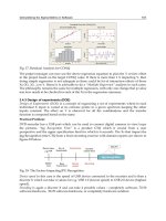
occurs together with test 5 failure on X chart.
d)
a)
R chart
X chart X chart X chart
b) c)

Fig. 8. Decreasing linear trend test interpretation

d)
a)
R chart
X chart X chart X chart
b) c)

Fig. 9. Increasing linear trend test interpretation


As so, according to the interpretations given, we are able to define the following function:
φ: {Run-Test Failures}  {Process Changes}
“detected anomalies” “what happens”

SPC Theory Process Changes

Run-Test
Failure
Process Performance

Type What Happens
None In Control None Nothing
RT1 Out of Control Occasional

Early Alarm
RT2
Out of Control
Occasional

Early Alarm
RT3
Out of Control
Occasional

Early Alarm
RT4
Out of Control
Occurred New Mean
RT5
Out of Control Occurred Increased Variability
RT6 Out of Control Occurred
Decreased
Variability
RT7
Out of Control
Occurred

New Sources of
Variability
RT8 Out of Control Ongoing
Ongoing
Phenomena
Table 2. Run-Test Interpretation Details.

For each run-test failure, φ is able to relate the “detected anomalies” to “what happens”
within the process and suggest their cause.

3.4 Tuning Sensibility
SPC control limits need to be recalibrated according to relevant process performance
changes. The sensibility of the monitoring activity has to be tuned continuously. The risk of
not tuning sensibility is to miss anomalies as the result of using larger limits than necessary
or having several false alarms.
 The monitoring activity based on SPC is carried out with control limits as baselines
within which the process can vary randomly. Process is monitored according to
specific characteristics (known as measurement objects) selected by the manager.
 Even when control limits are well estimated they can become obsolete due to
process performance changes.
 Control limits are too tight, too wide, or the central line is no longer representative
of the average process performances.
 Measurement object is no longer representative, the measures used may no longer
express process variability.
In both cases it is necessary to:
1. identify when a relevant process performance change occurs;
2. tune the control model (i.e. recalibrate control limits) according to performance
changes.
Point (1) follows from the experience acquired during empirical validation of the SPC
approach in a previous study (Baldassarre et al., 2004). Following to this experience we have

generalized a set of relations between “what happens” in the process and what the best
actions to undertake are (Table 3).

Process Changes
Tuning Actions
Type What Happens
None Nothing No Action
Occasional Early Alarm No Action
Occurred New Mean Identify new control limits (new reference set)
Occurred Increased Variability Identify new control limits (new reference set)
Occurred Decreased Variability Identify new control limits (new reference set)
Occurred New Sources of Variability

Identify a new measurement object
Ongoing Ongoing Phenomena No Action
Table 3. Relationship between Process Changes and the necessary SPC Tuning Actions.

According to such relations and to “Process Changes” described through the “run-test
interpretation” we have defined the following function:

ψ: {Process Changes}  {Tuning Actions}
“what happens” “what to do”

Statistical Process Control for Software: Fill the Gap 149

induced process improvement, such as the introduction of a new technology, or a
spontaneous one, such as the maturation effect. This test, give insightful remarks when it
fails on R chart and it is interpreted jointly between X and R charts. For example:
 If R chart shows a decreasing trend as in Figure 8(d), a possible interpretation is that
the process is going asymptotically towards a new stability point: better as in Figure

8(b) or worse than actual Figure 8(a). If this is the case, this test failure should be
followed by a limit test failure (typically test 4) on X chart. Another situation is
represented in Figure 8(c) i.e. a process is going towards a more stable situation
around the central line, after a strong period of destabilization.
 If R chart shows an increasing trend, as in Figure 9(d), then the process is becoming
unstable, its performance are changing in a turbulent manner and it is far from
reaching a new point of stability (see as in Figure 9(a, b, c). Typically this test failure
occurs together with test 5 failure on X chart.
d)
a)
R chart
X chart X chart X chart
b) c)

Fig. 8. Decreasing linear trend test interpretation

d)
a)
R chart
X chart X chart X chart
b) c)

Fig. 9. Increasing linear trend test interpretation


As so, according to the interpretations given, we are able to define the following function:
φ: {Run-Test Failures}  {Process Changes}
“detected anomalies” “what happens”

SPC Theory Process Changes

Run-Test
Failure
Process Performance

Type What Happens
None In Control None Nothing
RT1 Out of Control Occasional

Early Alarm
RT2
Out of Control
Occasional

Early Alarm
RT3
Out of Control
Occasional

Early Alarm
RT4
Out of Control
Occurred New Mean
RT5
Out of Control Occurred Increased Variability
RT6 Out of Control Occurred
Decreased
Variability
RT7
Out of Control
Occurred

New Sources of
Variability
RT8 Out of Control Ongoing
Ongoing
Phenomena
Table 2. Run-Test Interpretation Details.

For each run-test failure, φ is able to relate the “detected anomalies” to “what happens”
within the process and suggest their cause.

3.4 Tuning Sensibility
SPC control limits need to be recalibrated according to relevant process performance
changes. The sensibility of the monitoring activity has to be tuned continuously. The risk of
not tuning sensibility is to miss anomalies as the result of using larger limits than necessary
or having several false alarms.
 The monitoring activity based on SPC is carried out with control limits as baselines
within which the process can vary randomly. Process is monitored according to
specific characteristics (known as measurement objects) selected by the manager.
 Even when control limits are well estimated they can become obsolete due to
process performance changes.
 Control limits are too tight, too wide, or the central line is no longer representative
of the average process performances.
 Measurement object is no longer representative, the measures used may no longer
express process variability.
In both cases it is necessary to:
1. identify when a relevant process performance change occurs;
2. tune the control model (i.e. recalibrate control limits) according to performance
changes.
Point (1) follows from the experience acquired during empirical validation of the SPC
approach in a previous study (Baldassarre et al., 2004). Following to this experience we have

generalized a set of relations between “what happens” in the process and what the best
actions to undertake are (Table 3).

Process Changes
Tuning Actions
Type What Happens
None Nothing No Action
Occasional Early Alarm No Action
Occurred New Mean Identify new control limits (new reference set)
Occurred Increased Variability Identify new control limits (new reference set)
Occurred Decreased Variability Identify new control limits (new reference set)
Occurred New Sources of Variability

Identify a new measurement object
Ongoing Ongoing Phenomena No Action
Table 3. Relationship between Process Changes and the necessary SPC Tuning Actions.

According to such relations and to “Process Changes” described through the “run-test
interpretation” we have defined the following function:

ψ: {Process Changes}  {Tuning Actions}
“what happens” “what to do”

Quality Management and Six Sigma150

Ψ is defined so that it assigns the appropriate tuning actions needed to update the SPC
settings preserving the sensibility of monitoring.
Thus ψ can be defined as follows:
 if the process change is “Occasional”, the process performance:
o should be the same as in the past if assignable causes have been detected

and removed or, if this is not the case, further observations are needed to
exhibit the new process performance;
o is probably changing due to the fact that assignable causes were made part
of the process. In this case further observations have to be collected.
In both cases the control limits and the measurement objects remain the same.
 if the process change is “Occurred”:
o if process mean or variability are changed then the control limits should
always be recalculated in order to determine a new reference set that
expresses the new process performance. The candidate points to be included
in the reference set are those responsible for the test failure.
o if there is a new source of variability then the different sources must be
identified, separated and tracked on different charts.
 if the process change is “Ongoing” additional observations are needed to
determine reliable limits for the process because the actual observations express a
change in actions and thus, they are not suitable for a reference set.
In this case “no action” is advisable.
Point (2) derives from composing functions φ and ψ, in ρ = ψoφ:
ρ: {Run-Test Failures}  {Tuning Actions}
“detected anomalies” “what to do”

ρ for each statistical “signal” suggests the suitable action to undertake to preserve
monitoring sensibility (Table 4).
Section 2, therefore, outlines a quick and effective solution that takes into account the issue
of process monitoring, allows to identify anomalies, suggests the most appropriate tuning
actions and preserves the monitoring model in use.

Run-Test Failure Tuning Actions
None No Action
RT1
No Action

RT2
No Action
RT3
No Action
RT4 Identify a new control limits
RT5 Identify a new control limits
RT6 Identify a new control limits
RT7 Identify a new measurement object
RT8 No Action
Table 4. Relationship between the Signals and the SPC Tuning Actions


Let us now apply these concepts to the explanatory figures 10 and 11. We can see that RT1,
RT2, and RT3 are classified as “occasional” process changes. They detect an early alarm, and
according to ψ do not require any tuning action. On the other hand, RT4 and RT5 are
classified as “occurred” process changes because the process mean has changed (RT4) and
the process variability, considering the limits in use, has also increased (RT5) as can clearly
be seen in figure 10. Indeed, the observed data points, from 16 on, no longer fall within the
fixed limits. Consequently, in accordance to ψ and to the guidelines in table 4, new control
limits must be calculated. Figure 11 shows the result of the tuning action, i.e. the new control
limits calculated from data points 16-30.

Fig. 10. RT4 and RT5 suggesting a shift in
process performances
Fig. 11. new control limits calculated from
data points 16-30

4. Discussion and final remarks
The presented framework, starting from the analysis of the Statistical Process Control as
commonly used in the manufacturing contexts, and based on the issues that characterize

software production, presents a set of evolutions and improvements that allow to:

 take into account the trends of observations rather than exclusively considering,
single data points, even if anomalous. Indeed, in software and in human intensive
processes, the behavioural trends are more significant than the single observations.
Furthermore, in software, a single event such as an observation that falls outside
the limits is not as critical as an observation in the manufacturing context. Indeed,
in the latter case, an observation out of the limits is most likely an indicator that
leads to discarding part of the production and stopping the production chain to
avoid further relevant economical losses. Fortunately, in software it is possible to
“rework” rather than discard the work already produced. The framework
presented in this paper on one hand implies Run Tests that focus on a long-
sequence of events (Limit and Trend tests) and, on the other, reinterprets the Run
Tests based on a short-sequence (Sigma Test) reorganizing them in meaning and
effect.
 make up for the lacks of SPC in the investigation phase of the anomalies and in
identifying appropriate interventions to make the monitored process stable again.
In this sense, it foresees a function φ that, based on the anomalies detected by the
Run-Tests, determines what happens in the process, i.e. identifies the changes
Statistical Process Control for Software: Fill the Gap 151

Ψ is defined so that it assigns the appropriate tuning actions needed to update the SPC
settings preserving the sensibility of monitoring.
Thus ψ can be defined as follows:
 if the process change is “Occasional”, the process performance:
o should be the same as in the past if assignable causes have been detected
and removed or, if this is not the case, further observations are needed to
exhibit the new process performance;
o is probably changing due to the fact that assignable causes were made part
of the process. In this case further observations have to be collected.

In both cases the control limits and the measurement objects remain the same.
 if the process change is “Occurred”:
o if process mean or variability are changed then the control limits should
always be recalculated in order to determine a new reference set that
expresses the new process performance. The candidate points to be included
in the reference set are those responsible for the test failure.
o if there is a new source of variability then the different sources must be
identified, separated and tracked on different charts.
 if the process change is “Ongoing” additional observations are needed to
determine reliable limits for the process because the actual observations express a
change in actions and thus, they are not suitable for a reference set.
In this case “no action” is advisable.
Point (2) derives from composing functions φ and ψ, in ρ = ψoφ:
ρ: {Run-Test Failures}  {Tuning Actions}
“detected anomalies” “what to do”

ρ for each statistical “signal” suggests the suitable action to undertake to preserve
monitoring sensibility (Table 4).
Section 2, therefore, outlines a quick and effective solution that takes into account the issue
of process monitoring, allows to identify anomalies, suggests the most appropriate tuning
actions and preserves the monitoring model in use.

Run-Test Failure Tuning Actions
None No Action
RT1
No Action
RT2
No Action
RT3
No Action

RT4 Identify a new control limits
RT5 Identify a new control limits
RT6 Identify a new control limits
RT7 Identify a new measurement object
RT8 No Action
Table 4. Relationship between the Signals and the SPC Tuning Actions


Let us now apply these concepts to the explanatory figures 10 and 11. We can see that RT1,
RT2, and RT3 are classified as “occasional” process changes. They detect an early alarm, and
according to ψ do not require any tuning action. On the other hand, RT4 and RT5 are
classified as “occurred” process changes because the process mean has changed (RT4) and
the process variability, considering the limits in use, has also increased (RT5) as can clearly
be seen in figure 10. Indeed, the observed data points, from 16 on, no longer fall within the
fixed limits. Consequently, in accordance to ψ and to the guidelines in table 4, new control
limits must be calculated. Figure 11 shows the result of the tuning action, i.e. the new control
limits calculated from data points 16-30.

Fig. 10. RT4 and RT5 suggesting a shift in
process performances
Fig. 11. new control limits calculated from
data points 16-30

4. Discussion and final remarks
The presented framework, starting from the analysis of the Statistical Process Control as
commonly used in the manufacturing contexts, and based on the issues that characterize
software production, presents a set of evolutions and improvements that allow to:

 take into account the trends of observations rather than exclusively considering,
single data points, even if anomalous. Indeed, in software and in human intensive

processes, the behavioural trends are more significant than the single observations.
Furthermore, in software, a single event such as an observation that falls outside
the limits is not as critical as an observation in the manufacturing context. Indeed,
in the latter case, an observation out of the limits is most likely an indicator that
leads to discarding part of the production and stopping the production chain to
avoid further relevant economical losses. Fortunately, in software it is possible to
“rework” rather than discard the work already produced. The framework
presented in this paper on one hand implies Run Tests that focus on a long-
sequence of events (Limit and Trend tests) and, on the other, reinterprets the Run
Tests based on a short-sequence (Sigma Test) reorganizing them in meaning and
effect.
 make up for the lacks of SPC in the investigation phase of the anomalies and in
identifying appropriate interventions to make the monitored process stable again.
In this sense, it foresees a function φ that, based on the anomalies detected by the
Run-Tests, determines what happens in the process, i.e. identifies the changes
Quality Management and Six Sigma152

occurred or taking place. As so, focused and specific actions can be identified and
carried out in order to regain a stable process.
 adapt the sensibility of monitoring actions with respect to the actual performances
of the monitored process. This characteristic is particularly important in pursuing
the effectiveness of monitoring. The current literature does not present useful
guidelines for determining when the control limits should be recalculated, in that
they are no longer representative of the process performances. Consequently an
incorrect use of SPC occurs, based on inadequate control limits which lead to
ineffective monitoring and control actions: too wide limits do not allow to
promptly raise significant variations, while too narrow ones determine numerous
false alarms. The proposed framework foresees the ψ function that associates
Tuning Actions, expression of “what to do”, to Process Changes, the expression of
“what happens”. This assures a dynamic and continuous calibration of monitoring

based on the actual observed process performances.
The framework represents an alternative to other software process monitoring techniques,
which can generally be considered as based on expert judgment, use measures collected in
time, and subject to subjective evaluations. In this sense, it is interesting to point out that the
framework:
 makes it possible to characterize process performances, even without having any
previous knowledge, by determining a reference set through a deterministic
procedure. Note that lack of previous knowledge usually occurs for innovative
processes, or for processes that are used in different contexts with different
maturity levels, or refer to various application domains (technical rather than
business). Moreover, in our framework, control limits are not an expert-based
estimation, but an actual expression of the process itself.
 provides a conceptual manner for defining process anomalies and, at the same
time, an operational means for identifying them. Without such instruments
(conceptual and operational) the interpretation of a trend rather than a single
observation would completely rely on the project manager, who may not
necessarily have the previous knowledge needed and thus, may neglect important
events or focus on irrelevant ones resulting in ineffective monitoring.
 represents an objective rather than subjective tool, a clear reference point, follows
rom explicit reasoning and based on a solid theoretic model (SPC).

Nevertheless, software process monitoring still represents an open issue. As discussed in
(Baldassarre et al., 2007), there are many aspects related to software process measurement
such as the difficulty of collecting metrics, their reliability and the selection of monitored
process characteristics (Sargut & Demirors, 2006); the violation of assumptions underlying
SPC (Raczynski & Curtis, 2008); predominance of human factors in software processes that
can impact on the SPC-theory and monitoring effectiveness [17]. All these aspects leave
much space for subjective management decisions that can influence the success/failure of
monitoring activities. Given these limitations, this framework is not intended as the solution
to monitoring problems, nor as a silver bullet for applying SPC to software processes.

Rather, it should be considered as a perspective on how SPC can contribute to practically
solve some monitoring issues according to the authors’ experience from the trench in real
industrial software projects. It can be seen as a contribution for guiding practitioners

towards a more disciplined use of SPC starting from understanding how it can really
address software process monitoring. In this way operational, practical issues and pitfalls of
SPC can be faced more systematically.

5. References
AT&T. (1956). “Statistical quality control handbook”, Indianapolis, AT&T Technologies,
1956
Baldassarre, M.T.; Boffoli, N.; Caivano, D. & Visaggio, G. (2005). Improving Dynamic
Calibration through Statistical Process Control. In: 21st International Conference on
Software Maintenance, pp. 273-282. IEEE Press, Budapest Hungary (2005)
Baldassarre, M.T.; Boffoli, N.; Bruno, G. & Caivano, D. (2009). International Conference on
Software Process, ICSP 2009 Vancouver, Canada, May 16-17, 2009 Proceedings.
Lecture Notes in Computer Science 5543 Springer 2009, ISBN 978-3-642-01679-0
Baldassarre, M.T.; Boffoli, N. & Caivano, D. (2008). Statistical Process Control for Software: a
Systematic Approach. In Proceedings of the Second International Symposium on
Empirical Software Engineering and Measurement, ESEM 2008, October 9-10, 2008,
Kaiserslautern, Germany. ACM 2008, ISBN 978-1-59593-971-5
Baldassarre, M.T.; Boffoli, N.; Caivano, D. & Visaggio, G. (2004). Managing Software Process
Improvement (SPI) through Statistical Process Control (SPC). In: 5th International
Conference on Product Focused Software Process Improvement, pp. 30-46. LNCS
Springer, Kansai Science City Japan (2004)
Baldassarre M.T.; Caivano D.; Kitchenham B. & Visaggio G. (2007). Systematic Review of
Statistical Process Control: an Experience Report. In: 11th International Conference
on Evaluation and Assessment on Software Engineering, pp.119-129. BCS, Keele
UK (2007)
Basili, V. R.; Caldiera, G. & Rombach, H.D. (1994). “Goal Question Metric Paradigm”,

Encyclopedia of Software Engineering, Vol. 1, John Wiley & Sons, 1994, pp. 528-532.
Boffoli, N. (2006). Non-Intrusive Monitoring of Software Quality. In: 10th European
conference on Software Maintenance and Reengineering, pp. 319-322. IEEE Press,
Bari Italy (2006)
Caivano, D. (2005). Continuous Software Process Improvement through Statistical Process
Control. In: 9th European Conference on Software Maintenance and Reengineering,
pp. 288-293. IEEE Press, Manchester UK (2005)
Card, D. (1994). Statistical Process Control for Software. IEEE Software, May 1994 pp. 95-97.
IEEE Press (1994)
Duncan, A. J. (1986). Quality Control and Industrial Statistics, R.D.IRWIN 5th edition, 1986
Ebenau, R.G. (1994). “Predictive Quality Control with Software Inspections”, Crosstalk, June
1994
Eickelmann, N. & Anant, A. (2003). Statistical Process Control: What You Don’t Measure
Can Hurt You! IEEE Software, Mar. /Apr. 2003, pp. 49-51. IEEE Press (2003)
Florac, W. A.; Carleton, A.D. & Bernard, J.R. (2000). “Statistical Process Control: Analyzing a
Space Shuttle Onboard Software Process”, IEEE Software, pp. 97-106, July/Aug.
2000.