Energy Storage Part 9 potx
Bạn đang xem bản rút gọn của tài liệu. Xem và tải ngay bản đầy đủ của tài liệu tại đây (529.93 KB, 13 trang )
Multi-Area Frequency and Tie-Line Power Flow Control by Fuzzy Gain Scheduled SMES
95
system frequency but the system oscillates for longer times. Decreasing the value of K
I
yields comparatively higher maximum frequency deviation at the beginning but provides
very good damping in the later cycles. These initiate a variable K
I
, which can be determined
from the frequency error and its derivative. Obviously, higher values of K
I
is needed at the
initial stage and then it should be changed gradually depending on the system frequency
changes.
Fig. 7. Frequency deviation step response for different values of K
I
Dynamic performance of the AGC system would obviously depend on the value of
frequency bias factors,
β
1
= β
2
=B and integral controller gain value, K
I1
=K
I2
=K
I
. In order to
optimize B and K
I
the concept of maximum stability margin is used, evaluated by the eigen-
values of the closed loop control system.
For a fixed gain supplementary controller, the optimal values of K
I
and B are chosen, here,
on the basis of a performance index (PI) given in (10) for a specific load change. The
Performance Index (PI) curves are shown in Fig. 8 without considering governor dead-band
(DB) and generation rate constraints (GRC).
()
T
222
tie 1 1 2 2
0
PI ΔPwΔfwΔfdt=++
∫
(10)
Where, w
1
and w
2
are the weight factors. The weight factors w
1
and w
2
both are chosen as
0.25 for the system under consideration [Sheikh et al., 2008].
From Fig. 8, in the absence of DB & GRC it is observed that the value of integral controller
gain, K
I
= 0.34 and frequency bias factors, B=0.4 which occurs at PI = 0.009888.
0 2 4 6
8
10 12
-8
-6
-4
-2
0
2
4
6
x
10
-4
Time [sec]
Frequency deviation [Hz]
K
I
=0
K
I
=1
Energy Storage
96
0.1 0.2 0.3 0.4 0.5 0.6
0.0095
0.01
0.0105
0.011
0.0115
0.012
0.0125
0.013
Integral Gain (K
I
)
Performance Index (PI)
B=0.1
B=0.15
B=0.2
B=0.25
B=0.3
B=0.35
B=0.4
B=0.45
B=0.5
Without GRC and Gov. Deadband
K
I
=0.34 and B=0.4 at PI=0.0099
Fig. 8. The optimal integral controller gain, K
I
and frequency bias factor, B
6. Control system design
6.1 Fuzzy gain schedule PI controller for AGC [Sheikh et al., 2008]
Figure 9 shows the membership functions for PI control system with a fuzzy gain scheduler.
The approach taken here is to exploit fuzzy rules and reasoning to generate controller
parameters. The triangular membership functions for the proposed fuzzy gain scheduled
integral (FGSPI) controller of the three variables (e
t
,
t
ce
, K
I
) are shown in Fig. 9, where
frequency error (e
t
) and change of frequency error (
t
ce
) are used as the inputs of the fuzzy
logic controller. K
Ii
is the output of fuzzy logic controller. Considering these two inputs, the
output of gain K
Ii
is determined. The use of two input and single output variables makes the
design of the controller very straightforward. A membership value for the various linguistic
variables is calculated by the rule given by
(
)
(
)
(
)
μ e,ce =minμ e,μ ce
tt t t
⎡
⎤
⎣
⎦
(11)
The equation of the triangular membership function used to determine the grade of
membership values in this work is as follows:
()
(
)
b-2 x-a
Ax=
b
(12)
Where A(x) is the value of grade of membership, ‘b’ is the width and ‘a’ is the coordinate of
the point at which the grade of membership is 1 and ‘x ‘ is the value of the input variables.
The control rules for the proposed strategy are very straightforward and have been
developed from the viewpoint of practical system operation and by trial and error methods.
Multi-Area Frequency and Tie-Line Power Flow Control by Fuzzy Gain Scheduled SMES
97
The membership functions, knowledge base and method of defuzzification determine the
performance of the FGSPI controller in a multi-area power system as shown in (13).
Mamdani’s max-min method is used. The center of gravity method is used for
difuzzification to obtain K
I
. The entire rule base for the FGSPI controller is shown in Table I.
n
μ u
jj
j=1
K=
n
I
μ
j
j=1
∑
∑
(13)
Fig. 9. Membership functions for the fuzzy variables
e
ce
NB NS Z PS PB
NB PB PB PB PS Z
NS PB PB PS Z NS
Z PB PS Z NS NB
PS PS Z NS NB NB
PB Z NS NB NB NB
Table 1. Fuzzy Rule base for FGSPI Controller
μ
[e
t
(x)]
NB NS Z PS PB
μ
[de
t
(x)/dt]
NB NS Z PS PB
μ
[K
Ii
(x)]
NB NS Z PS PB
-0.1 -0.05 0 0.05 0.1 e
t
(x)
1 0.75 0.32 0.01 0.001 K
I
(x)
-0.03 -0.015 0 0.015 0.03 de
t
(x)/dt
1
1
1
Energy Storage
98
6.2 Control strategy for SMES
Figure 10 outlines the proposed simple control scheme for SMES, which is incorporated in
each control area to reduce the instantaneous mismatch between the demand and
generation, where I
sm
, V
sm
and P
sm
are SMES current, SMES voltage and SMES power
respectively. For operating point change due to load changes, gain (K
Ii
) scheduled
supplementary controller is proposed. Firstly K
Ii
is determined using the fuzzy controller to
obtain frequency deviation,
Δf, and tie-line power deviation, ΔPtie. Finally ACE
i
which is the
combination of
ΔPtie and Δf [as shown in (9)] is used as the input to the SMES controller. It
is desirable to restore the inductor current to its rated value as quickly as possible after a
system disturbance, so that the SMES unit can respond properly to any subsequent
disturbance. So inductor current deviation is sensed and used as negative feedback signal in
the SMES control loop to achieve quick restoration of current and SMES energy levels.
Fig. 10.
Superconducting magnetic energy storage unit control system
7. Simulation results
To demonstrate the usefulness of the proposed controller, computer simulations were
performed using the MATLAB environment under different operating conditions. The
system performances with gain scheduled SMES and fixed gain SMES are shown in Fig. 11
through Fig. 14. Two case studies are conducted as follows:
Case I: a step load increase (ΔP
L2
=0.01 pu) is considered in area2 only.
It is seen from Fig. 11 that, the tie line power deviation are more reduced with the proposed
gain scheduled controller than the fixed gain one including SMES, and the deviations are
positive in Case I. Thus sensing the input signal ACE
i
in both the control areas SMES
provide sufficient compensation as shown in Fig. 12, where in area1 SMES is
charging/discharging energy and area2 SMES is discharging/charging energy to keep the
frequency deviations in both areas minimum. From Fig. 12 it is seen that, fuzzy gain
scheduled integral controller of the loaded area determines the integral gain, K
I
, to a
scheduled value to resotore the frequency to its nominal value, and fuzzy gain scheduled
integral controller of the unloaded area reamains unscheduled and selects the critical value
dc
0
sT1
K
+
dc
id
sT1
K
+
sLR
1
L
+
Δ
I
sm
I
sm
Δ
V
sm
Δ
V
sm
P
sm
ACE
i
Π
+-
+
+
I
sm0
V
sm0
+
V
sm
+
+
+
Multi-Area Frequency and Tie-Line Power Flow Control by Fuzzy Gain Scheduled SMES
99
0 5 10 15
-1
0
1
2
3
4
x 10
-3
Time [sec]
Tie-power deviation [pu MW]
Gain Scheduled+SMES
Fixed gain+SM ES
Fig. 11. Performances of tie power deviation for a step load increase ∆P
L2
=0.01 pu in area2
only
-0.01
-0.008
-0.006
-0.004
-0.002
0
A
rea-
1
Frequency deviation [Hz]
Gain Scheduled+SM ES
Fixed gain+SM ES
-0.015
-0.01
-0.005
0
A
rea-
2
Gain Scheduled+SM ES
Fixed gain+SMES
0
0.5
1
Ki Variation
0.2
0.4
0.6
0.8
1
4.85
4.9
4.95
Ism deviation [kA]
3.5
4
4.5
5
0 5 10 15
-4
-2
0
2
4
6
x 10
-4
Psm [MW]
Time [sec]
0 5 10 15
-6
-4
-2
0
2
x 10
-3
Time [sec]
Fig. 12. System performances for a step load increase ∆P
L2
=0.01 pu in area2 only
Energy Storage
100
0 5 10 15
-2.5
-2
-1.5
-1
-0.5
0
0.5
1
x 10
-3
Time [sec]
Tie-power deviation [pu MW]
Gain Scheduled+SM ES
Fixed gain+SM ES
Fig. 13. performances of tie power deviation for a step load increase ∆P
L1
=0.015 pu in area1
& ∆P
L2
= 0.01 pu in area2
-0.03
-0.025
-0.02
-0.015
-0.01
-0.005
0
Area-1
Frequency deviation [Hz]
Gain Scheduled+SMES
Fixed gain+SM ES
-0.03
-0.025
-0.02
-0.015
-0.01
-0.005
0
Area-2
Gain Scheduled+SMES
Fixed gain+SMES
0.2
0.4
0.6
0.8
1
Ki Variation
0.2
0.4
0.6
0.8
1
2.5
3
3.5
4
4.5
5
Ism deviation [kA]
3.5
4
4.5
5
0 5 10 15
-10
-5
0
5
x 10
-3
Psm [MW]
Time [sec]
0 5 10 15
-6
-4
-2
0
2
x 10
-3
Time [sec]
Fig. 14. System performances for a step load increase ∆P
L1
=0.015 pu in area1 & ∆P
L2
= 0.01 pu
in area2
Multi-Area Frequency and Tie-Line Power Flow Control by Fuzzy Gain Scheduled SMES
101
as its integral gain. In addition, it is seen that, the damping of the system frequency is not
satisfactory in the case with the fixed gain controller including SMES, but the proposed gain
scheduled supplementary controller including SMES significantly improves the system
performances.
Case II: different step load increase is applied to each area.
In this case, as each area is loaded by the different load increase, each area adjusts their own
load. Fig. 13 shows the tie power deviation but the magnitude is small. So the SMES
controller in both areas dominated on
Δf
i
. As ΔP
L1
=0.015 pu & ΔP
L2
=0.01 pu, it is seen from
Fig. 14 that SMES in area1 provided more compensation than that in area2. The inductor
current deviation (
ΔI
sm
) is also reduced significantly and return back to the rated value
quickly with the proposed control system. Finally, it is seen from Fig. 14 that fuzzy gain
scheduled integral controller of both the loaded areas determine the integral gain K
Ii
to a
scheduled value to resotore the frequency to its nominal value. Due to this, the damping of
the system frequency is also improved with the proposed FGSPI controller including SMES.
8. Chapter conclusions
The chapter discussed about the simulation studies that have been carried out on a two-area
power system to investigate the impact of the proposed intelligently controlled SMES on the
improvement of power system dynamic performances. The results clearly show that the
scheme is very powerful in reducing the frequency and tie-power deviations under a variety
of load perturbations. On-line adaptation of supplementary controller gain associated with
SMES makes the proposed intelligent controllers more effective and are expected to perform
optimally under different operating conditions.
9. References
Benjamin, NN. & Chan, WC. (1978). Multilevel Load-frequency Control of Inter-Connected
Power Systems,
IEE Proceedings, Generation, Transmission and Distribution,Vol.
No.125, pp.521–526.
Nanda, J. & Kavi, BL. (1988). Automatic Generation Control of Interconnected Power
System,
IEE Proceedings, Generation, Transmission and Distribution, Vol. 125, No. 5,
pp.385–390.
Das, D.; Nanda, J.; Kothari, ML. & Kothari, DP. (1990). Automatic Generation Control of
Hydrothermal System with New Area Control Error Considering Generation Rate
Constraint,
Electrical Machines and Power System, Vol. 18, pp.461–471.
Mufti, M. U.; Ahmad Lone, S.; Sheikh, J. I. & Imran, M. (2007). Improved Load Frequency
Control with Superconducting Magnetic Energy Storage in Interconnected Power
System,
IEEJ Transactions on Power and Energy, Vol. 2, pp. 387-397.
Nanda, J.; Mangla, A & Suri, S. (2006). Some New Findings on Automatic Generation
Control of an Interconnected Hydrothermal System with Conventional Controllers,
IEEE Transactions on Energy Conversion, Vol. 21, No. 1, pp. 187-194, (March, 2006).
Oysal, Y.; Yilmaz, A.S. & Koklukaya, E. (2004). Dynamic Fuzzy Networks Based Load
Frequency Controller Design in Electrical Power Systems,
G.U. Journal of Science,
Vol. 17, No. 3, pp. 101-114
Benjamin, NN. & Chan WC. (1982). Variable Structure Control of Electric Power Generation.
IEEE Transactions on Power Apparatus and System, Vol. 101, No. 2, pp.376–380.
Energy Storage
102
Sivaramaksishana, AY.; Hariharan, MV. & Srisailam, MC. (1984). Design of Variable
Structure Load-Frequency Controller Using Pole Assignment Techniques,
International Journal of Control, Vol. 40, No. 3, pp.437–498.
Tripathy, SC, & Juengst, KP. (1997). Sampled Data Automatic Generation Control with
Superconducting Magnetic Energy Storage,
IEEE Transactions on Energy Conversion
Vol. 12, No. 2, pp.187–192.
Shayeghi, H. & Shayanfar, H.A. (2004). Autometic Generation Control of Interconnected
Power System Using ANN Technique Based on
μ-Synthesis, Journal of Electrical
Engineering
, Vol. 55, No. 11-12, pp. 306-313.
Sheikh, M.R.I.; Muyeen, S.M.; Takahashi, R.; Murata, T. & Tamura, J. (2008). Improvement of
Load Frequency Control with Fuzzy Gain Scheduled Superconducting Magnetic
Energy Storage Unit,
International Conference of Electrical Machine (ICEM, 08), (06-09
September, 2008), Vilamura, Portugal.
Demiroren, A. (2002). Application of a Self-Tuning to Automatic Generation Control in
Power System Including SMES Units,
European Transactions on Electrical Power, Vol.
12, No. 2, pp. 101-109, (March/April 2002).
IEEE Task Force on Benchmark Models for Digital Simulation of FACTS and Custom–Power
Controllers, T&D Committee, (2006). Detailed Modeling of Superconducting
Magnetic Energy Storage (SMES) System,
IEEE Transactions on Power Delivery, Vol.
21, No. 2, pp. 699-710, (April 2006).
Ali, M. H.; Murata, T. & Tamura, J. (2008). Transient Stability Enhancement by Fuzzy Logic-
Controlled SMES Considering Coordination with Optimal Reclosing of Circuit
Breakers,
IEEE Transactions on Power Systems, Vol. 23, No. 2, pp. 631-640, (May 2008).
2grp/energystorage_report/node8.html
Demiroren, A. & Yesil, E. (2004). Automatic Generation Control with Fuzzy Logic
Controllers in the Power System Including SMES Units,
International Journal of
Electrical Power & Energy Systems, Vol. 26, pp. 291-305.
Abraham, R.J.; Das, D. & Patra, A. (2008). AGC Study of a Hydrothermal System with SMES
and TCPS,
European Transactions on Electrical Power, DOI: 10.1002/etep.235
Wu, C. J. & Lee, Y. S. (1991). Application of Superconducting Magnetic Energy Storage to
Improve the Damping of Synchronous Generator,
IEEE Transactions on Energy
Conversion, Vol. 6, No. 4, pp. 573-578, (December 1991).
Banerjee, S.; Chatterjee, J. K. & Tripathy, S. C. (1990). Application of Magnetic Energy
Storage Unit as Load Frequency Stabilizer,
IEEE Transactions on Energy
Conversion, Vol. 5, No. 1, pp. 46-51, (March 1990).
M.R.I. Sheikh was born in Sirajgonj, Bangladesh on October 31, 1967. He
received his B.Sc. Eng. and M.Sc. Eng. Degree from Rajshahi University of
Engineering & Technology (RUET), Bangladesh, in 1992 and 2003
respectively, all in Electrical and Electronic Engineering. He is currently an
Associate Professor in the Electrical and Electronic Engineering Department,
RUET. Presently he is working towards his Ph.D Degree at the Kitami
Institute of Technology, Hokkaido, Kitami, Japan. His research interests are, Power System
Stability Enhancement Including Wind Generator by Using SMES, FACTs devices and Load
Frequency Control of multi-area power system.
Mr. Sheikh is the member of the IEB and the BCS of Bangladesh.
6
Influence of Streamer-to-Glow
Transition on NO Removal by Inductive
Energy Storage Pulse Generator
Koichi Takaki
Iwate University
Japan
1. Introduction
Huge amounts of air pollutants like carbon monoxide, unburned hydrocarbons, nitrogen
oxides (NOx), and particulate matter have been released into the atmosphere by various
sources such as coal, oil, and natural gas-burning electric power generating plants, motor
vehicles, diesel engine exhaust, paper mills, metal and chemical production plants, etc., over
the last several decades. These pollutants are the main cause of acid rain, urban smog, and
respiratory organ disease (Chang, 2001). For pollutants emitted from motor vehicle, the
exhaust of gasoline engines is cleaned effectively with the three-way catalyst. However, for
diesel and lean burn engines, the three-way-catalyst does not work because the high oxygen
content in the exhaust gases prevents the reduction of nitrogen oxide (NO) (Clements et al.,
1989).
Dry NOx removal technology is one of the conventional processes which may provide a
potential solution for such problems (Eliasson and Kogelschatz, 1991). A non-thermal
plasma process using a pulse streamer corona discharge is particularly attractive for this
purpose (Namihira et al., 2000). During the past decade, numerous studies on this process
have been conducted using a diesel engine exhaust gas and/or a simulated gas (Hackam &
Akiyama, 2000). Although encouraging results have been obtained from the experiments, it
is urgent to design a whole removal system compact enough for vehicle application.
Two methods for storing energy are employed in high-power pulse generators: capacitive
and inductive storages. When the energy is stored in capacitors, the energy is transferred to
a load through closing devices, e.g., high-current nanosecond switches. If the energy is
stored in an inductive circuit with current, opening switch is used to transfer energy to a
load (Rukin, 1999). For short-pulsed high voltage generation with high impedance load,
inductive energy storage (IES) system is more adequate than capacitive energy storage
system, if appropriate opening switches are available (Jiang et al., 2007).
High-voltage nanosecond pulse generators, in which high-voltage semiconductor diodes are
employed for interrupting currents stored as inductive energy, have been developed (Rukin,
1999). The generators using the high-voltage diodes as semiconductor opening switch (SOS)
have an all-solid-state switching system and therefore, combine high pulse repetition rate,
stability of the output parameters and long lifetime (Grekhov & Mesyats, 2002). SOS pulse
generators operating at various institutions demonstrated their high reliability during
Energy Storage
104
applied research work connected with the pumping of gas lasers (Baksht et al., 2002),
ionization of air with a corona discharge (Yalandin, et al., 2002, Cathey, et al., 2007),
generation of radical species with a atmospheric pressure glow discharge (Takaki, et al.,
2005), and generation of high-power microwave (Bushlyakov et al., 2006).
The streamer discharges driven by a pulsed power generator can dissociate oxygen
molecules to atomic oxygen radicals with high-energy efficiency because of low-conductive
current loss (Fukawa et al., 2008). The IES pulsed power generator using SOS diodes is
particularly attractive for this purpose because the whole system can be compact,
lightweight and driven at high repetition rate. However, a discharge produced by the IES
pulsed power generator transients from streamer to glow when the energy stored in the
capacitor still remains after the energy transfer from a capacitor to an inductor at opening
the SOS diodes (Grekhov & Mesyats, 2002). As the results, the energy efficiency for gas
treatment using non-thermal plasma is affected by the streamer-to-glow transition (Takaki
et al., 2007). In here, NO removal using a co-axial type non-thermal plasma reactor driven
by an IES pulsed power generator is described. The influence of streamer-to-glow transition
on NO removal in the non-thermal plasma reactor is also described.
2. Experimental setup
Figure 1(a) shows the schematics of the experimental circuit. The IES pulsed power
generator consists of a primary energy storage capacitor C, a closing switch SW, a secondary
energy storage inductor L, and an opening switch. The circuit current flows to the LC circuit
governed by the following equation after closing the switch SW (Robiscoe et al., 1998):
0
2
0
0
sin
R
t
L
V
ie t
L
ω
ω
−
= , (1)
2
0
1
2
R
LC L
ω
⎛⎞
=−
⎜⎟
⎝⎠
, (2)
where t is the time from the activation of the closing switch, V
0
is the charged voltage, L is
the inductance of the energy storage inductor, C is the capacitance of the primary energy
storage capacitor, and R is the circuit resistance (R < 4 L / C). When SOS diodes are used as
an opening switch as shown in Figure 1(a), the circuit current flows through the SOS diodes
as a forward-pumping current during a half period
F
TLC
π
≈ of LC oscillation (Yalandin
et al., 2000). After the current direction reverses with LC oscillation, the reverse current is
injected into the SOS during the period
T
R
. After the injection phase T
R
, the circuit current is
interrupted by a short duration
T
O
. With the current interrupted by the SOS, a high-voltage
pulse is produced as follows:
0
1
out
di di
VV idtL RiL
Cdt dt
=− − −≈−
∫
, (3)
as shown in Fig. 1(b). This pulse voltage can be applied to a load as a short nanosecond
pulse (Takaki et al., 2005, Rukin, 1999, Yankelevich & Pokryvailo, 2002).
Influence of Streamer-to-Glow Transition on NO Removal
by Inductive Energy Storage Pulse Generator
105
SOS
diode
L
C
V
out
I
0
0
0
S W
TF
TR TO
V
0
t
t
(a)
(b)
V
out
I
0
Fig. 1. Schematic of an inductive energy storage pulse power generator with semiconductor
opening switch: (a) equivalent circuit; (b) circuit current and output voltage.
Fast reverse recovery diodes VMI K100UF (Voltage Multipliers, Inc., 10 kV maximum
voltage, 100 A maximum current,
T
R
=100 ns) were employed as SOS diodes, i.e., a
semiconductor opening switch. K100UF diodes were connected in 5 series and 4 parallel to
decrease the circuit inductance and to increase capable forward pumping current and
reversed voltage (400 A maximum current, 50 kV maximum voltage). The capacitance of the
primary energy storage capacitor
C and the inductance of the secondary energy storage
inductor
L were changed in range from 0.12 to 4.2 nF and from 4.8 to 18.5 μF, respectively,
as shown in
Table 1. The charging voltages of the capacitor C were -20 kV for conditions 1-3
and -12 kV for condition 4. The pulse repetition rate was changed to control the input
energy in the reactor. The current and voltage were measured with Pearson 2878 current
transformers (0.1 V/A sensitivity, 400 A maximum current, 5 ns rise time) and Tektronix
high-voltage P6015A probe (40 kV peak voltage, 4 ns rise time), respectively. The signals
stored in a Tektronix TDS3054B digitizing oscilloscope (500 MHz band width, 5 GS/s
sampling rate) was transmitted to a computer through a LAN cable for calculating the
energy consumed in reactor.
Condition #1 #2 #3 #4
C [nF] 0.12 0.23 0.48 4.2
L [μH] 18.5 10.5 4.8 12.6
T
F
[ns] 203 205 224 876
T
R
[ns] 67 68 69 102
Table 1. Forward and reversed pumping time of SOS diodes for various circuit parameters.
Figure 2 shows a schematic of the experimental set-up using the pulse streamer discharge
reactor. The simulated gas was diluted NO with nitrogen and oxygen mixed with ratio of
9:1. The co-axial plasma reactor consists of a 1mm
φ tungsten wire and a copper cylinder
Energy Storage
106
Inlet
V
o u t
I
D
O 2
NO
+
N
2
V C I 0
controler
Flow
outlet
Gas Analyzar
Coaxial Reactor
Mixture
Vessel
Fig. 2. Experimental setup for NO removal from simulated exhaust gas using a corona
discharge reactor driven by an IES pulse power generator.
with an inner diameter of 20 mm. The length of the reactor is 300 mm, which corresponds to
94 cc in volume. The initial concentration of NO gas was controlled to 200 ppm using a mass
flow controller. The flow rate of the simulated gas was changed from 2 to 4 L/min. The NO
and NO
2
gases were analyzed by Best Sokki BCL-511 gas analyzer.
3. Results and discussion
3.1 Pulse power circuit behavior
Figure 3
shows typical waveforms of circuit current I
0
, capacitor voltage V
C
, and output
voltage
V
out
without connecting to the load at C=0.48 nF and L=4.8 μH. The charging voltage
V
0
of the capacitor C is -10 kV. “Time = 0” means the time after closing the gap switch SW.
The circuit current
I
0
starts to flow after closing the gap switch SW with LC oscillation. The
diode forward-pumping period
T
F
, i.e., a half period of LC oscillation, is 210 ns, and the
peak of the forward-pumping current is 67 A. After the current direction reverses with LC
oscillation, the reverse current is injected into the SOS during a 70 ns period
T
R
. After the 70
ns injection phase
T
R
, the circuit current is interrupted for 25 ns duration T
O
. During this
phase, the 50 A reversed current is interrupted for 25 ns. The output voltage increases
rapidly and has a maximum voltage of 22 kV, which corresponds to 2.2 of an amplification
factor, i.e. corresponds to the ratio of the maximum output voltage to the charging voltage
V
0
. The pulse width of the output voltage is 25 ns in FWHM (full-width at half-maximum).
The total inductance of the circuit is the summation of the secondary energy storage
inductor and a circuit loop inductance. The total circuit inductance can be roughly estimated
using the equation
F
TLC
π
≈
and is calculated to be 9.6 μH using a 210 ns half period of
LC oscillation. This inductance and rapid current interruption produces a high voltage pulse
expressed by Equation (3).
Table 1 shows the periods of a forward-pumping current
T
F
and the periods of a reverse
current of the diodes
T
R
for various circuit conditions. The period T
F
has approximately
same values at around 200 ns (203, 205, and 224 ns for conditions 1, 2, and 3, respectively)
for all three different conditions. The period
T
F
can be predicted as a half cycle of LC
oscillation and was calculated to be 146, 154, and 150 ns using values of
C and L of the
conditions 1, 2, and 3, respectively. The measured period
T
F
shows a larger value than those
Influence of Streamer-to-Glow Transition on NO Removal
by Inductive Energy Storage Pulse Generator
107
0 0.1 0.2 0.3
-30
-20
-10
0
10
20
30
-80
-40
0
40
80
Time [μs]
Voltage [kV]
Current [A]
I
0
V
C
V
out
T
F
T
R
C =0.48 nF
L
=4.8 μH
Fig. 3. Typical waveforms of circuit current
I
0
, capacitor voltage V
C
, and output voltage V
out
without connection to the load at
C=0.48 nF, L=4.8 μH and V
0
=-10 kV.
calculated by the result of a stray inductance of the circuit. The reverse current period
T
R
has
approximately the same values for different circuit conditions in the same forward current
period. However, the value of
T
R
is around 70 ns which is 70% of the rated period of 100 ns.
The values of
L and C in condition 4 were chosen to increase the forward-current period T
F
as
723LC
π
= ns. The obtained period of T
R
is 102 ns, which agreed well with the rated
period of 100 ns.
Figure 4 shows the typical time-dependency of the discharge current I
load
, the circuit current
I
0
, the reactor voltage V
out
and the voltage of the primary energy storage capacitor V
C
with
connection of the pulsed power generator to the reactor. The circuit condition is chosen as
C=0.68 nF and L=1.4 μH. The charging voltage V
0
of the capacitor is set to be -20 kV. The
discharge current
I
load
can be divided by two parts; displacement current at the early part of
the current and a discharge current as the sharp peak. The peak value of the discharge
current is around 100 A. The voltage of the capacitor
V
C
is almost zero when the pulse
voltage is produced and applied to the reactor. This result indicates the energy stored in the
capacitor is almost released through LC oscillation.
Figure 4 also shows time-dependency of energy stored in the secondary energy storage
inductor
E
L
, energy stored in the primary energy storage capacitor E
C
, energy loss in the
SOS diodes
E
SOS
and energy consumed in the reactor E
load
. The energy stored in the
capacitor is transferred to the inductor in the period of first quarter cycle of the LC
oscillation. After that, the energy stored in the inductor is transferred back to the capacitor
in next quarter cycle. The energy of 16 mJ is consumed in the SOS in the period of LC half
cycle because of the resistive component of the SOS diodes. The total energy transfer from
the primary energy storage capacitor to the reactor is around 20% under the circuit
condition. The energy transfer efficiency changes by changing circuit parameter as reported
in the reference (Takaki et al., 2007). The energy transfer efficiency increases to 40% by
decreasing circuit current from 200 to 50 A in peak value because the energy loss in the SOS
decreases with decreasing current through the SOS diodes.