A finite difference method using high order schemes for modeling non linear chromatography
Bạn đang xem bản rút gọn của tài liệu. Xem và tải ngay bản đầy đủ của tài liệu tại đây (3.51 MB, 107 trang )
VIET NAM NATIONAL UNIVERSITY HO CHI MINH CITY
HO CHI MINH UNIVERSITY OF TECHNOLOGY
CAO HÀ THÀNH
A FINITE DIFFERENCE METHOD USING
HIGH – ORDER SCHEMES FOR MODELING
NON – LINEAR CHROMATOGRAPHY
PHƯƠNG PHÁP SAI PHÂN HỮU HẠN SỬ DỤNG
CÔNG THỨC BẬC CAO ĐỂ MÔ PHỎNG
SẮC KÝ PHI TUYẾN TÍNH
Major: Chemical Engineering
Major ID: 8520301
MASTER’S THESIS
HO CHI MINH CITY, February 2023
This research was completed in: Ho Chi Minh university of Technology. VN HCM
Thesis supervisor: (Signature)
Assoc. Prof. PhD. Nguyen Tuan Anh
Reviewer 1: (Signature)
Assoc. Prof. PhD. Nguyen Quang Long
Reviewer 2: (Signature)
PhD. Ly Cam Hung
Master’s Thesis was defended in HCMC University of Technology, VNU-HCM on
February 14th, 2023.
The participants of the Mater’s Thesis Defend Council includes:
1. Chairman: Assoc. Prof. PhD. Nguyen Đinh Thanh
2. Reviewer 1: Assoc. Prof. PhD. Nguyen Quang Long
3. Reviewer 2: PhD. Ly Cam Hung
4. Participant: PhD. Đang Bao Trung
5. Secretary: PhD. Đang Van Han
Verification of the chairman of the Master’s Thesis Defense Council the Head of
Chemical Engineering Faculty.
CHAIRMAN OF THE COUNCIL
DEAN OF CHEMICAL ENGINEERING FACULTY
(Full name and Signature)
(Full name and Signature)
ii
Vietnam National University HCMC
SOCIALIST REPUBLIC OF VIETNAM
HCM University of Technology
Independent - Librety- Hapiness
MASTER’S THESIS ASSIGNMENT
Full name: Cao Ha Thanh
Student ID: 1970161
Date of birth: 08/01/1996
Place of birth: TP.HCM
Major : Chemical Engineering
Major ID : 8520301
I. TITLE
A FINITE DIFFERENCE METHOD USING HIGH – ORDER SCHEMES FOR
MODELING NON – LINEAR CHROMATOGRAPHY
PHƯƠNG PHÁP SAI PHÂN HỮU HẠN SỬ DỤNG CÔNG THỨC BẬC CAO ĐỂ
MÔ PHỎNG SẮC KÝ PHI TUYẾN TÍNH
II. ASSIGNMENT AND CONTENT
Establishing high- order approximation schemes to simulate HPLC
Verifying the schemes using relavent test functions
Applying the schemes in simulating the two major model of HPLC, namely GRM
and EDM
Analysing the effect of operation parameters on parameters of the
chromatographic peak
Validation by comparing the simulation and the experiments.
III. ASSIGNMENT DELIVERY DATE : 14/02/2022
IV. ASSIGNMENT COMPLETION DATE : 10/12/2022
V. THESIS SUPERVISOR : Assoc. Prof. PhD. Nguyen Tuan Anh
HCM city, _____________
THESIS SUPERVISOR
HEAD OF DEPARTMENT
(Full name and Signature)
(Full name and Signature)
DEAN OF CHEMICAL ENGINEERING FACULTY
(Full name and Signature)
iii
Acknowledgement
First and foremost, I would like to express my sincere gratitude to my thesis supervisor,
Associate Professor Dr. Nguyen Anh Tuan. In 2019, he taught me Modeling and
Simulation. Thanks to his inspiring teaching, I learned the miracle of the numerical
method, which can help engineers solve any differential equation. Since then, my
passion for discipline began to grow, and I decided to research this field. His
comprehensive expertise, extensive experience, and enthusiastic guidance are essential
factors in helping me do this research. Besides, I also appreciate the intellectual support
of my friend, Nguyen Van Vinh Ha. His experiments and knowledge in analytical
chemistry are valuable to me. And last but not least, I would like to thank all my friends,
family, and colleagues who have given me indispensable emotional support.
Lời cảm ơn
Đầu tiên, tôi xin gửi lời cảm ơn trân thành tới PGS. TS. Nguyễn Tuấn Anh, giảng viên
hướng dẫn luận văn này. Từ năm 2019, thầy Tuấn Anh đã dạy tơi mơn Mơ hình hóa và
Mơ phỏng. Nhờ và vào những bài giảng truyền cảm hứng của thầy, tôi đã thấy được sự
kỳ diệu của phương pháp số, thứ có thể giúp các kỹ sư giải được mọi phương trình. Từ
đó, niềm đam mê của tơi dành cho Mô phỏng lớn dần lên và tôi quyết định thực hiện
nghiên cứu theo hướng này. Chuyên môn và kinh nghiệm dày dặn trong lĩnh vực mô
phỏng cộng với sự hướng dẫn tận tình của thầy là những yếu tố then chốt giúp tôi thực
hiện được luận văn này. Bên cạnh đó, tơi cũng vơ cùng trân trọng sự giúp đỡ của bạn
Nguyễn Văn Vĩnh Hà. Các thí nghiệm của bạn cùng những góp ý chun mơn trong lĩnh
vực phân tích đã đóng vai trị khơng nhỏ trong việc giúp tơi hồn thành luận văn này.
Và cuối cùng nhưng cũng không kém phần quan trọng, tôi xin cảm ơn bạn bè, gia đình,
và đồng nghiệp, những người đã dành cho tôi sự ủng hộ tinh thần quý giá.
iv
Abstract
High – performance liquid chromatography (HPLC) is a dynamic separation process
with a lot of parameters having different roles. Operation parameters such as volume
fraction of organic modifier, column temperature, flow rate, etc. have significant effects
on system suitability presented by system suitability parameters such as plate count,
retention factor, symmetry factor, etc. One way to demonstrate this process is using the
model of the transportation of diluted species in porous media. The model gives an
equation of HPLC that illustrates the equilibrium state of analytes between the surface
of stationary phase particles and mobile phase, advection, and diffusion of analyte in the
mobile phase within the column. The solutions of the equation will indicate the effects
of operation parameters on the system suitability ones and can be used to predict the
behavior of a HPLC. Thus, the simulation of HPLC can give chemists a cutting-edge
tool for developing analytical methods. The equations can be solved by semi – analytical
methods, finite element methods, finite volume methods, or finite difference methods.
The finite difference methods are favorable for solving problems that involved flow.
This thesis was about defining the partial differential equation of HPLC which was
solved using a finite difference method. Taylor expansion is used in a general method
for defining scheme to approximate the derivatives, and the truncation errors of these
schemes. A fourth – order central difference scheme was used for estimating diffusion
while a fifth – order upwind schemes are used for modeling. The modeling of the PDE
equation runs on MATLAB script, which gives the model a great advantage of flexibility
and high degree of control on the mathematical algorithm. The model was evaluated by
assessing the area recovery of the peak, testing non – retained substance behavior and
comparing the calculation results with experimental data.
v
Tóm tắt
Sắc ký lỏng hiệu năng cao (HPLC) là một q trình phức tạp có nhiều thơng số vận hành
đóng các vai trị khác nhau. Các thơng số vận hành này gồm có tỉ lệ thể tích của dung
mơi hữu cơ trong pha động, nhiệt độ cột, tốc độ dòng, … có ảnh hưởng lớn tới kết quả
sự ổn định của hệ thống, được thể hiện qua các thông số tuong thích hệ thống như số đĩa
lý thuyết, thời gian lưu, hệ số đối xứng, … Q trình HPLC có thể được mơ hình hóa
bằng hiện tượng truyền vận của cấu tử nồng độ thấp trong mơi trường xốp. Nhóm mơ
hình này đưa ra các phương trình diễn tả mối quan hệ giữa nồng độ trong pha tĩnh và
pha động của chất pha tĩnh, sự dịch chuyển do dòng chảy của pha động và q trình
khếch tán. Mơ hình này, về lý thuyết, cung cấp các ảnh hưởng của các thông số vận hành
đối với các thông số của peak trong sắc ký đồ và là cơng cụ hữu ích để dự đốn và phát
triển các phương pháp phân tích sử dụng HPLC. Các phương trình này có thể được giải
bằng một số cách khác nhau như phương pháp giải tích, phương pháp phần tử hữu hạn,và
phương pháp sai phân hữu hạn. Trong đó phương thức sai phân hữu hạn có nhiều ưu
điểm phù hợp để giải bài tốn có liên qua đến dòng chảy như trường hợp của HPLC.
Trong luận văn này, các phương trình vi phân riệng phần để mô phỏng HPLC sẽ được
thiết lập và được giải bằng một phương pháp sai phân hữu hạn. Khai triển Taylor được
dùng để thiết lập các công thức sai phân để xấp xỉ các phép đạo hàm và xác định sai số
của các công thức xấp xỉ này. Một công thức đối xứng bậc 4 dùng để xấp xỉ hiện tượng
khếch tán và một công thức bậc 5 được dùng để xấp xỉ dịng chảy. Việc mơ phỏng được
thực hiện bằng code MATLAB để thuận tiện cho việc kiểm soát thuật toán và dễ dàng
áp dụng các thay đổi khi cần thiết. Mơ hình được thẩm định bằng cách kiểm tra bảo tồn
vật chất, mơ phỏng peak của chất khơng có tương tác và so sánh với kết quả thực nghiệm.
vi
Declaration
I proclaim that this thesis is original and that any other source is cited appropriately.
Most of the figures in this work are originally illustrated, and the others are adapted
from the identified source.
Lời cam đoan
Tôi xin cam kết luận văn này là nguyên bản, tất cả các tài liệu tham khảo khác đều được
trích dẫn đúng cách và ghi nguồn cụ thể. Các hình ảnh số liệu phần lớn được lấy từ kết
quả của luận văn này, các hình ảnh từ nguồn khác đều được trích dẫn phù hợp.
(Ký tên)
Cao Hà Thành
vii
Contents
MASTER’S THESIS ASSIGNMENT .......................................................................... iii
Acknowledgement ......................................................................................................... iv
Lời cảm ơn ..................................................................................................................... iv
Abstract ........................................................................................................................... v
Tóm tắt ........................................................................................................................... vi
Declaration .................................................................................................................... vii
Lời cam đoan ................................................................................................................ vii
List of figures ................................................................................................................. xi
List of tables ................................................................................................................. xiii
Notation and glossary .................................................................................................. xiv
List of Abbreviations .................................................................................................. xvii
Chapter 1: Literature review......................................................................................... 1
1.1. HPLC simulation ............................................................................................... 1
1.1.1. HPLC simulation: data – driven methods .................................................. 1
1.1.2. Theory – based approaches for HPLC simulation...................................... 5
1.2. Finite difference methods ................................................................................ 10
1.3. Other studies .................................................................................................... 11
1.4. Relevance and motivation ............................................................................... 13
Chapter 2: Simulation and Modeling ......................................................................... 14
2.1. Model assumptions .......................................................................................... 14
2.2. Modeling ......................................................................................................... 14
2.2.1. Mass conservation equation ..................................................................... 14
2.2.2. Adsorption models.................................................................................... 17
2.2.3. Calculating porosity.................................................................................. 21
viii
2.2.4. Calculating diffusion coefficient .............................................................. 21
2.3. Simulation ....................................................................................................... 22
2.3.1. Deriving approximation schemes for first order derivatives .................... 22
2.3.2. Deriving approximation schemes for second order derivatives ............... 27
2.3.3. Injection simulation .................................................................................. 29
2.3.4. Courant number and alpha number .......................................................... 29
2.3.5. Central difference scheme for diffusion ................................................... 30
2.3.6. Approximation of derivative of concentration with respect to distance in
the Equilibrium Dispersive Model ........................................................................ 30
2.3.7. Approximation of derivative of concentration with respect to distance in
the General Rate Model ......................................................................................... 35
2.3.8. Approximation of derivative of concentration with respect to time ........ 36
Chapter 3: Calculation and Experiment ..................................................................... 37
3.1. Software and codes .......................................................................................... 37
3.2. Chemicals and equipment ............................................................................... 37
3.3. Scheme’s verification ...................................................................................... 37
3.4. Experiment ...................................................................................................... 39
Chapter 4: Results and discussions ............................................................................ 40
4.1. Verification of the schemes’ accuracy ............................................................ 40
4.1.1. Derivative of the surface concentration.................................................... 40
4.1.2. Derivative of concentration in the mobile phase ...................................... 43
4.2. Simulation result.............................................................................................. 44
4.2.1. Distribution of the analyte in the column ................................................. 44
4.2.2. Effect of Approximation schemes ............................................................ 46
4.2.3. Effect of diffusion coefficient .................................................................. 49
4.2.4. Effect of mass transfer coefficient ............................................................ 51
ix
4.2.5. Effect of capacity of the stationary phase................................................. 52
4.2.6. Effect of adsorption constant .................................................................... 54
4.2.7. Effect of flow rate ..................................................................................... 56
4.2.8. Effect of injection concentration .............................................................. 57
4.2.9. Effect of injection volume ........................................................................ 58
4.2.10.
Multi – component separation............................................................... 59
4.3. Model validation.............................................................................................. 61
4.3.1. Assessment of mass conservation ............................................................ 61
4.3.2. Simulation of non – retained substance. ................................................... 62
4.3.3. Single injection ......................................................................................... 62
4.3.4. Simulation of a sample set ........................................................................ 64
Chapter 5: Conclusions .............................................................................................. 70
List of Publication ......................................................................................................... 71
References ..................................................................................................................... 72
Appendix A:
Algorithm to define approximation schemes ..................................... 78
Appendix B:
Algorithm for validating schemes to approximate derivative of
adsorption constant ....................................................................................................... 79
Appendix C:
Algorithm for validating schemes to approximate derivative of
concentration
81
Appendix D:
Verification results the approximation schemes ................................ 88
BIOGRAPHY ............................................................................................................... 90
STUDY EXPERIENCE ................................................................................................ 90
WORKING EXPERIENCE .......................................................................................... 90
x
List of figures
Figure 1.1: HPLC model classification........................................................................... 1
Figure 2.1: HPLC diagram ............................................................................................ 14
Figure 2.2: Effect of the isotherm curve on the peak shape (recreated from [44])....... 17
Figure 2.3: Procedure of derivative calculation ............................................................ 20
Figure 2.4: Injection pulse ............................................................................................ 29
Figure 4.1: Test function and the respective verification results .................................. 40
Figure 4.2: Relative error and logarithm of relative error as functions of ∆C ............. 41
Figure 4.3: Verification result of different test function with different n0................... 42
Figure 4.4: Distribution of concentration in the column using EDM ........................... 44
Figure 4.5: Distribution of concentration in the column using GRM........................... 45
Figure 4.6: Chromatogram and suitability parameters at different approximation scheme
for simulating the derivative of concentration with respect to distance in linear range
using GRM .................................................................................................................... 46
Figure 4.7: Chromatogram at different approximation scheme for simulating the
derivative of concentration with respect to distance in non – linear range using GRM
....................................................................................................................................... 47
Figure 4.8: Chromatogram and suitability parameters at different approximation scheme
for simulating the derivative of concentration with respect to time in linear range using
GRM ............................................................................................................................. 48
Figure 4.9: Chromatogram and suitability parameters at different diffusion coefficients
using EDM .................................................................................................................... 49
Figure 4.10: Chromatogram and suitability parameters at different diffusion coefficients
using GRM .................................................................................................................... 50
Figure 4.11: Chromatogram and suitability parameters at different mass transfer
coefficient using GRM .................................................................................................. 51
Figure 4.12: Chromatogram and suitability parameters at different capacity of the
stationary phase using EDM ......................................................................................... 52
Figure 4.13: Chromatogram and suitability parameters at different capacity of the
stationary phase using GRM ......................................................................................... 52
xi
Figure 4.14: Chromatogram and suitability parameters at different adsorption constant
using EDM .................................................................................................................... 54
Figure 4.15: Chromatogram and suitability parameters at different adsorption constant
using GRM .................................................................................................................... 54
Figure 4.16: Area recovery of peaks produced by the EDM and GRM ....................... 55
Figure 4.17: Chromatogram and suitability parameters at different flow rate using GRM
....................................................................................................................................... 56
Figure 4.18: Chromatogram and suitability parameters at different injection
concentrations in linear range using GRM ................................................................... 57
Figure 4.19: Chromatogram and suitability parameters at different injection
concentrations outside linear range using GRM ........................................................... 57
Figure 4.20: Chromatograms and suitability parameters at different injection volumes in
linear range using GRM ................................................................................................ 58
Figure 4.21: Chromatograms and suitability parameters at different injection volumes
outside linear range using GRM ................................................................................... 58
Figure 4.22: Chromatograms of multi – component separation with similar
concentrations using GRM ........................................................................................... 59
Figure 4.23: Chromatograms of multi – component separation with different
concentrations using GRM ........................................................................................... 60
Figure 4.24: Experiment and simulation result at Vinj = 10 µL using GRM ................ 62
Figure 4.25: Retention time of experiment and simulation using EDM....................... 64
Figure 4.26: Peak widths of experiment and simulation using EDM ........................... 64
Figure 4.27 : Symmetry factor of experiment and simulation using EDM .................. 65
Figure 4.28: Plate count of experiment and simulation using EDM ............................ 65
Figure 4.29: Retention time of experiment and simulation using GRM ...................... 66
Figure 4.30: Peak widths of experiment and simulation using GRM........................... 66
Figure 4.31: Symmetry factor of experiment and simulation using GRM ................... 67
Figure 4.32: Plate count of experiment and simulation using GRM ............................ 67
Figure D.1: Verification result of the schemes used for simulating advection ............ 88
Figure D.2: Verification result of the schemes used for simulating diffusion ............. 89
xii
List of tables
Table 2.1: Approximation for first order derivatives.................................................... 26
Table 2.2: Approximation for second order derivatives ............................................... 28
Table 3.1: Chemical reagent’s information .................................................................. 37
Table 3.2: Experimental parameters ............................................................................. 39
Table 4.1: Area recovery of the simulation peak using EDM ...................................... 61
Table 4.2: Area recovery of the simulation peak using GRM ...................................... 61
Table 4.3: SST parameters of the experiment and simulation peak using EDM.......... 63
Table 4.4: SST parameters of the experiment and simulation peak using GRM ......... 63
Table 4.5: Experiment and simulation results using EDM ........................................... 68
Table 4.6: Simulation accuracy and bias of the system suitability parameters using EDM
....................................................................................................................................... 68
Table 4.7: Experiment and simulation results using GRM........................................... 69
Table 4.8: Simulation accuracy and bias of the system suitability parameters using GRM
....................................................................................................................................... 69
Table D.1: The schemes used for simulating advection ............................................... 88
Table D.2: The schemes used for simulating diffusion ................................................ 89
xiii
Notation and glossary
Character
Unit
Description
Ac
𝑚
An
-
Asp
𝑚
Ap
-
Approximation result of the scheme
AR
%
Area recovery of the peak
As
-
Symmetry factor
C
𝑚𝑜𝑙/𝑚
Concentration of analyte in mobile phase
Cinj
𝑚𝑜𝑙/𝑚
Injection concentration
Cr
-
D
𝑚 /𝑠
dp
𝑚
Diameter of stationary phase particle
EI
-
Error index
Er
-
Error of the approximation
F
𝑚 /𝑠
i, j
-
Co – Ordinator
ID1
𝑚
Internal diameter of the guard column
ID2
𝑚
Internal diameter of the column
k’
-
Retention factor
KF
-
Freundlich adsorption constant
KL
𝑚 /𝑚𝑜𝑙
Langmuir adsorption constant
KL1, KL2
𝑚 /𝑚𝑜𝑙
Bi – Langmuir adsorption constant
L1
𝑚
Length of the guard column
L2
𝑚
Length of the column
Ma
𝑔/𝑚𝑜𝑙
Molar mass of the analyte
MMP
𝑔/𝑚𝑜𝑙
Average molecular weight of the mobile phase
Morg
𝑔/𝑚𝑜𝑙
Molecular weight of the organic modifier
N
-
Cross sectional area of the inner column
Analytical result of the test function
Surface area of stationary phase particle
Courant number
Diffusion coefficient
Flow rate of the mobile phase
Number of segments that given the concentration 𝐶
xiv
Character
Unit
Description
n
𝑚𝑜𝑙/𝑚
Concentration of analyte on the surface of stationary
phase
n0
𝑚𝑜𝑙/𝑚
Monolayer capacity of stationary phase
NEP
-
nsat
𝑚𝑜𝑙/𝑚
NUSP
-
nvoid
𝑚𝑜𝑙/𝑚
r
-
RE
-
RT
min
RT0
𝑠
sp
𝑚 ⁄𝑚
TC
℃
Column temperature
tinj
𝑠
Injection time
tvoid
𝑠
System void volume
u1
𝑚/𝑠
Linear velocity of mobile phase in guard column
u2, u
𝑚/𝑠
Linear velocity of mobile phase in column
VC
𝑚
Volume of column limited by dx
Vinj
𝑚
Injection volume
Vm
𝑚𝐿/𝑚𝑜𝑙
Vp
𝑚
wd
s
Wd10
min
Peak width at 10 % height
Wd5
min
Peak width at 5 % height
WdUSP
min
USP tangent peak width
zMP
-
EP plate count
Saturated concentration on surface of stationary phase’s
surface
USP plate count
Concentration of empty space on stationary phase’s
surface
Ratio of the amount of analyte in stationary phase and
mobile phase
Relative error of the scheme compared to the analytical
result
Retention time
Retention time of an analyte that is not adsorbed by
stationary phase
Specific surface area of stationary phase particle
Molar volume of the analyte
Volume of stationary phase particle
Standard deviation of the injection pulse
Solvent association parameter
xv
Character
Unit
Description
zorg
-
Mobile phase association parameter of the organic
modifier
α
-
Alpha number
β
1/𝑠
γ
𝑚 /𝑚
ε
-
η
𝑚𝑃𝑎. 𝑠
Mobile phase viscosity
θ
𝑚 /𝑚
Ratio of stationary phase surface area to mobile phase
volume
λ
-
ρa
𝑔⁄𝑚𝐿
Analyte density
ρp
𝑘𝑔⁄𝑚
Density of stationary phase particle
ϕ
-
Mass transfer coefficient
Saturated distribution coefficient
Porosity of stationary phase particle
Modifying factor of extended Langmuir isotherm
Volume fraction of the organic modifier
xvi
List of Abbreviations
ANFIS
Adaptive – neuro fuzzy inference system
ANN
Artificial neural network
EDM
Equilibrium dispersive model
EP
European Pharmacopeia
FDM
Finite difference method
FEM
Finite element method
FVM
Finite volume method
GRM
General rate model
HPLC
High performance liquid chromatography
IDQC HCM
Institute of Drug Quality Control – Ho Chi Minh City
LC
Liquid chromatography
MAPE
Mean absolute percentage error
MLP – ANN
Multiple layer perceptron artificial neural network
MLR
Multiple linear regression
MSE
Mean – squared error
ODE
Ordinary differential equations
OOA
Order of accuracy
PDE
Partial differential equations
QSRR
Quantitative structure – retention relationships
RMSE
Root mean – squared error
SST
System Suitability Test
USP
United States Pharmacopeia
xvii
Chapter 1:
1.1.
Literature review
HPLC simulation
HPLC models
Theoretical
Plate models
Theory based
methods
Data -driven
methods
General Rate
models
Equilibrium
Dispersive
models
Numerical
methods
Finite
difference
methods
Analytical
methods
Finite element
methods
Figure 1.1: HPLC model classification
1.1.1. HPLC simulation: data – driven methods
There are numerous studies and software using empirical data to interpret the relationship
between operation parameters and retention time, peak width, etc. [1] [2] [3] [4] [5] [6] [7]
In 2013, Paul G. Boswell and his colleges proposed an HPLC simulator as an effective
educational tool for a student studying analytical chemistry. [1]The study was based on
experimental data of 22 compounds on an Agilent Zorbax SB – C8 column in both gradient
and isocratic mode. Fundamental principles of HPLC were demonstrated in several
1
empirical equations which were used to calculate retention time, peak width from operation
parameters like temperature, mobile phase composition, flow rate, injection volume,
column length, and diameter, etc. Chromatograms featured with Gaussian peaks could be
plotted for each compound. These equations were coded into an HPLC simulator in Java
programming language. The study also tested the effectiveness of the HPLC model as an
educational tool for undergraduate analytical chemistry students. The result shown that
students who had been given access to the simulator outperformed those who hadn’t (score
12.5/15 compared to 11.7/15) in the quiz to assess their understanding of HPLC
fundamental principles. [1] Despite many achievements, there was room for improvement.
For instance, the simulator did not give students information about the symmetry factor
which was quite important as a system suitability parameter. The simulator used was
limited for educational purposes because it could not predict retention time and peak width
of a novel compound besides the 22 ones in the library.
An artificial neural network was used in another study in 2019 by Angelo Antonio
D’Archivio. [2] The ANN – based model illustrated the elution data of 16 derivatives of
amino acids under organic modifier gradients (φ gradient), pH gradients, and double φ/pH
gradients. Empirical data obtained from the three original pieces of literature of Pappa
Louisi and co–workers [1] [8] [9]. The data provided a massive amount of information
about the effect of solvent strength, pH, the combination of both on retention behavior. The
mobile phases used in these experiments were mixtures of acetonitrile and aqueous
phosphate buffer with a total ionic strength of 0.02 M. In the first study [1] 19
chromatograms were obtained from different fixed eluent pHs (between 2.80 and 7.80),
while the volume fraction of the organic modifier was linearly varied between 0.2 and 0.5
in several gradient durations. The dataset given by the second paper had the organic
modifier fraction fixed (at 0.25, 0.27, 0.3, or 0.35), and applied 22 different linear pH
gradients in the pH ranges of 2.8 –10.7 or 3.2 – 9. The third study achieved by Zisi applied
a double organic solvent and pH gradient. pH and organic solvent fraction were changed
simultaneously as a linear function. There were 27 different experiments implemented at
settled values of initial solvent fraction (0.25) and pH (3.21), while final gradient time, pH,
2
and solvent fraction were varied according to a three – level preliminary design. The chosen
final pH level was 4.68, 5.86, and 7.86; selected organic modifier fraction were 0.35, 0.40,
and 0.50; and 10, 20, and 30 min were the chosen gradient time. The data had been used to
calibrate the model which was applied to predict the retention behavior of these analytes in
reversed phase HPLC. Using ANN as a regression tool is an excellent way to build a high
accuracy model with coefficients of determination in training (R2) ranging from 0.9980 to
0.9999 and coefficients of determination in prediction (Q2) ranging from 0.9799 to 0.9984.
This model also provided a valuable prediction of retention time with mean error for pH
gradients were 1.4%, for organic modifier fraction gradients were 1.1% and for combined
pH/solvent gradients were 2.5%. [2] The model was very useful for predicting retention
time, but other system suitability parameters like symmetry factor, plate count, peak width,
etc., which are quite impactful in chromatography separation have not been studied yet.
In 2020, another study of S.I. Abba and his teams used artificial intelligence to simulate
HPLC in a data – driven approach. [10] There are three data – driven methodologies
proposed: artificial neural network (ANN), adaptive – neuro – fuzzy inference system
(ANFIS), and multi – linear regression (MLR). Different data – intelligence models were
applied to find out whether a specific approach could be more desirable than others in
producing reliable results. The models used pH and volume fraction of organic modifiers
(methanol) as key input parameters. Amiloride and methyclothiazide were chosen to model
their retention behavior and peak widths in ion chromatography (IC). Mobile phase
programs consisted of isocratic, gradient, and multistep gradients. Predictive results of
these models were evaluated by various statistical parameters include correlation
coefficient (R), coefficients of determination (R2), root mean – squared error (RMSE),
mean – squared error (MSE), and mean absolute percentage error (MAPE). Correlation
coefficients of ANN were 0.8977 and 0.9615; ANFIS were 0.9714 and 0.9568; MLR is
0.6613 and 0.8406 for training phase and ANN were 0.8794 and 0.9461; ANFIS were
0.9483 and 0.9774; MLR were 0.688 and 0.8668 in testing phase. [10] The results indicated
a superior of ANN and ANFIS over MLR, and ANFIS had a modest advantage compare to
3
ANN. The research is one of a few research implementing different data – intelligent
methods and comparing the results.
Quantitative structure – retention relationships are widely used in chemical and biology
research. [11] A study of Soo Hyun Park and co – workers used quantitative structure –
retention relationships (QSRR) to predict retention behavior of low molecular weight
anions in IC. [12] The model was based on the well – known equation log k’=a – b*log[E].
When k’ is the retention factor, [E] is the concentration of the eluent, values a and b are
respectively the intercept and the slope of the linear solvent strength model. The model
used evolutionary algorithm – multi linear regression (EA – MLR) to obtain a and b values
for small organic and inorganic ion. Evolutionary algorithms were inspired by Charles
Darwin’s theory of evolution. A set of proposed solutions were created for the problem.
These solutions were called ‘population’ and they will be evaluated by calculating a set of
parameters that indicate how good the solutions fit the reality. The so – called population
evolves over time in order to gain better solutions. [13] The QSRR model was used to
predict a and b of the novel molecules. These values in turn were used to predict the
retention behavior of the analytes. External validation shown a good agreement between
predicted retention time with experimental data. QSRR models have a remarkable
advantage over other data – driven methods which is the ability to predict the retention
behavior of analytes outside the existing databases.
Summary: data – based approaches are the most popular models for simulating HPLC. This
makes sense because of the high complexity of the principle of the HPLC system, which is
easy to describe yet extremely difficult to calculate. The techniques to interpret data such
as ANN, ANFIS, MLR, QSRR are diversified and constantly evolving. In the age of
progressively advancing information technology, data processing methods have an
enormous potential to evolve. However, these methods have difficulty in dealing with novel
analytes and require a massive amount of data, which is not always available for everyone.
4
1.1.2. Theory – based approaches for HPLC simulation
HPLC could be simulated by using physicochemical theories to formulate equations
demonstrating principles of fluid dynamics, adsorption, and diffusion. These equations are
partial differential equations (PDE) that could be solved by numerical or algebraical
methods. [14] [15] [16] [17] Another approach is creating an algorithm from theories to
calculate the desired parameters. [18] The advantage of these models is not being dependent
on a huge amount of experimental data, they just need minuscule number of experiments
for calibrating the model and validating the results.
1.1.2.1. Equilibrium – dispersive model
Equilibrium – dispersive model assumes that the concentration on the surface of stationary
phase and the concentration in the mobile phase get equilibrium immediately. Axial
dispersion and mass transfer resistances are considered negligible. These assumptions are
suitable for predicting the behavior of a high – performance system with insignificant mass
transfer resistance. HPLC and other high – resolution chromatography systems can be
simulated by this model. Retention time can be predicted by this model with meaningful
accuracy. However, it does not get sufficient precision in predicting the peak shape when
mass transfer resistances are considerable. [14] There are some studies and practical
applications using the equilibrium theory. [15] [19] [20] [21]
1.1.2.2. Plate model
The plate model is one of the fundamental principles for studying and modeling
chromatography. Plate models have two versions. The first type is equivalent to the tank –
in – series model for non – ideal flow systems. This approach conceptualizes the column as
a series of minuscule theoretical cells, each with complete mixing. The result is a series of
first–order ordinary differential equations (ODEs) demonstrating the adsorption and mass
transfer between the mobile phase and surface of stationary phase particles. [14] There were
a lot of researchers studying HPLC simulation, using this approach. [16] [22] [23] [24]
Defining the equilibrium of each compound in each theoretical cell by distribution
coefficient is the principle of the second type of plate model. Instead of solving ODE
5
systems, the solution is obtained by using recursive iterations. [14] Craig models are among
the most outstanding ones. The distribution Craig models can be applied to multi – analyte
systems by using the so – called blockage effect. [25] Column – overload problem can be
researched by using the Craig models. Velayudhan and Ladisch had elution and frontal
adsorption phenomenon simulated by a Craig model with a corrected plate count.
In 2011, J.J. Baeza – Baeza proposed a version of Martin and Synge plate model including
slow mass – transfer kinetics between the fluid phase and the particle phase. [16] The study
bases on the plate model dividing the HPLC column into N theoretical plates. This approach
allows the model to simulate the slow mass – transfer process throughout the column.
Laplace transform was used to solve the ODEs achieved from the model (one equation for
each theoretical plate). The model introduced a concept of kinetic ratio expressed by the
proportion of the kinetic constants for the mass transfer in the flow direction to the mass
transfer between the mobile phase and stationary phase. The study used an experimental
method to estimate drift from equilibrium conditions by variances and retention times at
different flow rates. Results imply a linear relationship between kinetic ratio and variance.
The greater the kinetic ratios are, the wider the peak widths are. On the other hand, the
faster flow rate had the variance of the peaks reduced. Validation was obtained by
comparing with the model of diluted species transfer through the theoretical plates, where
the mobile phase migrates from a theoretical plate to the next in modest steps, after that the
mobile phase is blended in completely. [16] The study has done a great job of applying
Laplace transform to solve the series of ODE obtained from the theoretical plate model.
An innovative algorithm modeling HPLC was proposed by Yaxiong Zhang in 2015. [18]
This model introduced a new coefficient called “phase transfer probability factor”
demonstrating the non – equilibrium distribution state. It also used genetic algorithm (GA)
to support the model in fitting simulated experimental data. Multiple layer perceptron
artificial neural networks (MLP – ANNs) and GA were the backing for simulating
separation process of the mixture samples containing phenol, hydroquinone, resorcinol, and
4 – nitrophenol. The study simulated HPLC column by dividing into N segments. The
6
equilibrium of each segment is identified by “phase transfer probability factor” and would
be used to calculate the concentration of analyte in mobile phase and stationary phase in
the next temporal increment. This recursive iteration method is the first type of theoretical
plate model. [14] This model can simulate non – linear and non – ideal analytical
chromatography.
1.1.2.3. Rate model
Rate model is an advanced version of equilibrium dispersive model, it considers the mass
transfer resistances between the mobile phase and the stationary phase. They often have
two or two set of equation, one presents the deviation of concentration in the mobile phase,
the other is for the stationary phase. [14] There are many studies and applications based on
rate models with various complexity. [14] [26] [27] [28] [29] [30] [31] [32]
A study in 2006 by P. Forssen [17] proposed an improved algorithm for gaining adsorption
factors by solving an inverse problem. The paper presented a numerical model using
experimental data to calibrate adsorption constant parameters. The work studied and
introduced improvements to the four fundamental parts of the algorithm used in the inverse
method. These are solving PDEs, calculating the Jacobian of the computer–simulated
chromatography data with adhering to the adsorption constant parameters, the
transformation of experimental chromatograms into concentration contributions, and
evaluating various potential adsorption constant models. The study applied the PDE solver
and Jacobian computation routine in Fortran 90 using Compaq Visual Fortran, Version 6.6
C. MATLAB Optimization Toolbox, Version 3.0. was used for optimizing the algorithm.
The study introduced several improvements in the proposed algorithm for the estimation of
adsorption constant parameters in liquid chromatography. These are to solve PDE using a
grid refinement procedure to reduce run time; a novel method for calculating Jacobian,
which is not only precise but also easily adjustable when being used for modeling
algorithm; using measured response functions to process experimental chromatogram data;
proposing a novel method to select the fittest adsorption constant function. [17] Despite the
outstanding performance in estimating adsorption constant, the model is quite old and has
7
some shortcomings. The model used a first – order scheme for approximating advection,
which is quite inaccurate. This error was reduced by using extremely small time and space
steps (∆t, ∆x) but this approach created another drawback – exceedingly long run time. The
study simply accepted the long run time as a minor inconvenience because they could have
their computer run overnight. However, this weakness can be overcome by using a higher
– order scheme to save run time without sacrificing accuracy.
A book written by Tingyue Gu in 2015 proposed a rate model to simulate and scale – up
liquid chromatography. [14] The book used rate models to simulate the elution of multi –
component samples in the LC column. The models not only investigated the main flow
direction diffusion, interfacial film mass transfer between the mobile phase and the surface
area of the stationary phase, but also inspected nonlinear multicomponent isotherms and
intraparticle dispersal. Several chromatographic processes like elution (including isocratic
and gradient mode), breakthrough, and displacement could be studied and predicted by
using the model. The book provides several models for simulating LC elution of organic
compounds (adsorption, reversed – phase, and hydrophobic interaction models), high
molecular weight compound (size – exclusion model), inorganic compound (ion –
exchange model), and protein (affinity model).
A study of Seemab Bashir and co – workers in 2017 used a linear general rate model to
simulate liquid chromatography reactor consisted of two compounds. [30] The model
examined first order reversible and irreversible reactions, linear kinetics of adsorption and
desorption, dispersion in axial direction, internal and external particle diffusions. These
phenomena were expressed in two set of differential equations. Laplace transform and
linear transformation were used to uncouple the mentioned set of equations resulting system
of separated ODEs. An elementary solution technique was employed to solve these OEDs.
The solutions in actual time domain were attained by applying the reversed numerical
Laplace transformation. Numerical solutions gained from high – resolution finite volume
scheme was used to validate the results. The semi – analytical solutions and the numerical
scheme were verified by considering different case studies. The study was successful in
8