Advances in Analog Circuits Part 7 docx
Bạn đang xem bản rút gọn của tài liệu. Xem và tải ngay bản đầy đủ của tài liệu tại đây (922.7 KB, 30 trang )
f = 0, the term δ( f ) |H( f )|
2
in (6) can be replaced with δ( f )H
2
(0)=δ( f )Q
2
,whereQ is the
charge transferred during the complete switching of a single logic gate:
Q
= H(0)=
+∞
−∞
h(t)dt.(7)
Therefore, the power spectral density S
I
( f ) of the stochastic process I(t) is:
S
I
( f )=λ
2
Q
2
δ( f )+λ ·|H( f )|
2
,(8)
and the normalized power P
I
of the switching current I(t) is:
P
I
=
+∞
−∞
S
I
( f )df = λ
2
Q
2
+ λ
+∞
−∞
|H( f )|
2
df.(9)
In (9), the term λ
2
Q
2
is the dc component of the digital switching power (λQ is the average
value of the current drawn from the supply voltage), while the term λ
+∞
−∞
|H( f )|
2
df is the
ac component of the switching power. The rightmost term in (9) can be simplified by using
Parseval’s theorem, thus obtaining:
P
I
= λ
2
Q
2
+ λ
+∞
−∞
h
2
(t)dt. (10)
For any impulse response h
(t), the normalized power P
I
can be written as:
P
I
= λ
2
Q
2
+ α
λ
t
p
Q
2
, (11)
where α is a “pulse shape” factor, which depends on the single current pulse waveform in
time domain, and t
p
is the switching time of logic gates (Boselli et al., 2010).
2.2 Current pulses with different duration, amplitude, and time density
Although equations (4) to (11) were derived starting from restrictive assumptions, the theory
can be extended to digital systems made of logic cells with different switching time, different
switching currents, and switching activity variable over time.
Let us start considering different switching times. For simplicity, let us assume that the
combinational circuit is made of two types of logic cells, labeled “A” and “B”. In more
detail, gates of type “A” are characterized by the digital switching current i
A
(t), which can
be described as a shot noise with time density λ
A
and impulse response h
A
(t),andgatesof
type “B” are characterized by the digital switching current i
B
(t), with time density λ
B
and
impulse response h
B
(t). The total current drawn by the whole circuit is:
i
(t)=i
A
(t)+i
B
(t), (12)
which is the sum of two shot noise processes. The amplitude distribution f
(i) of the total
current i
(t) is:
f
(i)= f
A
(i) ∗ f
B
(i), (13)
where f
A
(i) and f
B
(i) can be calculated separately using (5).
The power spectral density S
II
( f ) is given by the sum of the p.s.d. of the single processes and
their cross-spectra:
S
II
( f )=S
AA
( f )+S
BB
( f )+S
AB
( f )+S
BA
( f ). (14)
169
Analog Design Issues for Mixed-Signal CMOS Integrated Circuits
The cross-spectra S
AB
( f ) and S
BA
( f ) can be obtained by taking the Fourier transforms of the
cross-correlations R
AB
(τ) and R
BA
(τ), which are constant:
R
AB
(τ)=R
BA
(τ)=λ
A
λ
B
Q
A
Q
B
. (15)
Therefore, the cross-spectra S
AB
( f ) and S
BA
( f ) have a single component at f = 0:
S
AB
( f )=S
BA
( f )=λ
A
λ
B
Q
A
Q
B
δ( f ). (16)
By using (8) and (16) in (14), we obtain:
S
II
( f )=
(
λ
A
Q
A
+ λ
B
Q
B
)
2
δ( f )+λ
A
·|H
A
( f )|
2
+ λ
B
·|H
B
( f )|
2
. (17)
Therefore, at f
= 0 the power spectrum component is given by the square of the sum of dc
current; while at any frequency f
= 0, the power spectral density is given by the sum of the
power spectral densities of all shot noise components.
Current pulses having different peak amplitudes can be described by considering Poisson
impulses with different intensities, proportional to the current drawn by logic gates. The
mathematical model is a generalized Poisson process (Papoulis & Pillai, 2002), given by:
X
G
(t)=
∑
i
c
i
δ(t −t
i
), (18)
where c
i
is a random variable representing the amplitude of Poisson impulses, with mean μ
c
and standard deviation σ
c
. The autocorrelation R
G
X
(τ) is (Papoulis & Pillai, 2002):
R
G
X
(τ)=μ
2
c
λ
2
+(μ
2
c
+ σ
2
c
) · λδ(τ), (19)
and the power spectral density S
G
X
( f ) is given by the Fourier transform:
S
G
X
( f )=F(R
G
X
(τ)) = μ
2
c
λ
2
δ( f )+(μ
2
c
+ σ
2
c
) · λ. (20)
The current consumption I
G
(t) due to switching activity of logic gates with different current
intensities can be calculated by filtering the process X
G
(t) through the linear, time-invariant
system h
(t). The power spectral density S
G
I
( f ) is:
S
G
I
( f )=S
G
X
( f ) ·|H( f )|
2
= λ
2
Q
2
avg
δ( f )+λ(1 + σ
2
c
) ·|H( f )|
2
, (21)
where Q
avg
represents the average charge transferred during the switching transitions
(assuming μ
c
= 1).
Finally, let us consider a non-uniform distribution of logic switching activity over time. In
this situation, the switching noise can be described by a non-stationary stochastic process.
In a sequential network driven by a master clock, we can assume that the time density of
logic transitions is periodic, and therefore we have a cyclostationary shot noise. Although
the p.s.d. cannot be defined for a non-stationary process, it is possible to define a “mean
energy spectrum” which has frequency components similar to (8), plus discrete frequency
components at the master clock frequency and its harmonics.
170
Advances in Analog Circuitsi
V
DD
RL
I
v
on−chip
off−chip
Fig. 4. Equivalent circuit for bondwires.
2.3 Effects of parasitics on on-c hip supply voltages
Digital switching noise propagates from the digital to the analog section through both
interconnections and substrate. Therefore, realistic models of interconnections (including
package, bonding and on-chip parasitics) and substrate must be adopted for simulations.
Such models are inherently technology dependent. The model of couplings through package
interconnections strongly depends on the package. Therefore, the designer should use the
correct model of the production package. For the same reason, the use of different package
types for prototyping is not recommended, as parasitic effects can be very different. Substrate
models can also be very different. We can distinguish two major categories of substrates:
heavily-doped bulk with epitaxial layer, and lightly-doped substrate. The heavily-doped bulk
has a very low resistance and can be considered as a single node. Therefore, any disturbance
injected into the bulk propagates into the whole chip, irrespective of the distance. On the
other hand, the lightly-doped substrate is resistive, and the substrate resistance attenuates the
injected disturbance. Some fabrication technologies allow to insert a buried n-well, that can
be used for shielding purposes. Such differences must be considered during the design of
the chip. Moreover, the same circuit integrated in different technologies can behave in a very
different way from the point of view of robustness to crosstalk. Indeed, effects of substrate
parasitics put a severe limit on design portability. The results obtained in previous subsection
can be used to calculate the on-chip noise voltage is due both to digital switching currents and
to parasitic elements.
Let us start considering the simplified circuit shown in Fig. 4, where the current generator
models the digital switching noise source, and bondwire parasitics are modeled as series
inductance L and resistance R. The bondwire impedance Z is:
Z
= R + sL = R + j2π fL. (22)
The on-chip power supply v is affected by a noise voltage having the power spectral density:
S
V
( f )=S
I
( f ) ·|Z|
2
= λ
2
Q
2
R
2
δ( f )+λR
2
·|H( f )|
2
+ λ(2π)
2
L
2
f
2
·|H( f )|
2
. (23)
The normalized power P
V
of the switching noise affecting the on-chip voltage supply v is:
P
V
=
+∞
−∞
S
V
( f )df = λ
2
Q
2
R
2
+ λR
2
+∞
−∞
h
2
(t)dt + λL
2
+∞
−∞
h
2
(t)dt, (24)
wherewehaveusedParseval’stheoremforbothh
(t) and its time derivative h
(t).The
first two terms in (24), λ
2
Q
2
R
2
and λR
2
+∞
−∞
h
2
(t)dt, are the dc and ac components due to
the voltage drop across the parasitic resistance R.Thelastterm,λL
2
+∞
−∞
h
2
(t)dt,istheac
171
Analog Design Issues for Mixed-Signal CMOS Integrated Circuits
V
DD
R
w
C
w
v
I
LR
off−chip
on−chip
Fig. 5. Equivalent circuit for calculation of bondwire and substrate parasitic effects.
component due to the parasitic inductance L. By comparing the voltage spectral density and
power in (23) and (24) with the current spectral density and power in (8) and (9), we can
observe that the noise voltage terms due to the parasitic resistance R are similar to the noise
current terms, since the resistance R gives a proportional relationship between current and
voltage. On the other hand, the last term in (23) and (24) accounts for the inductive voltage
drop Lh
(t). Therefore, spectral characteristics of noise voltage are dependent on both the
impulse response h
(t) and its time derivative h
(t). The rms value of the on-chip noise voltage
is given by:
v
rms
=
P
V
=
λ
2
Q
2
R
2
+ λR
2
+∞
−∞
h
2
(t)dt + λL
2
+∞
−∞
h
2
(t)dt. (25)
Now we suppose that, besides bondwire parasitic inductance L and resistance R, the n-well
and p-substrate are providing an additional ac path from on-chip supply towards ground,
modeled by the resistance R
w
and the capacitance C
w
, as shown in Fig. 5. The overall
impedance Z is:
Z
=
R + s(L + RR
w
C
w
)+s
2
LR
w
C
w
1 + s(R + R
w
)C
w
+ s
2
LC
w
. (26)
Since the impedance formula (26) has a second-order denominator, oscillations may arise in
the circuit in the underdamped case, i.e., when
R
+ R
w
< 2
L
C
w
. (27)
If the values of parasitics satisfy (27), then the current pulses due to digital switching make the
on-chip voltage supply to oscillate, giving rise to the well known “VDD bounce”. The lower
the ratio
(R + R
w
)/
L
C
w
, the longer the duration of the bouncing.
2.4 Interconnection parasitics
An accurate model of interactions between analog and digital parts of an integrated circuit
must account for off-chip parasitics. In particular, package and wire bonding parasitics may
give a remarkable contribution to propagation of switching noise. Indeed, in addition to
the parasitic elements of a single interconnection, an accurate model should consider also
capacitances and mutual inductances between adjacent wires, as shown in Fig. 6 (Boselli
172
Advances in Analog Circuitsi
V
DD
LR
i
DD
(external) (on-chip)
V
DD
C
GND
KK
LR
v(t)
v
s
C
C
GND
LR
LR
Fig. 6. Equivalent circuit of bonding and package parasitics between two adjacent wires.
et al., 2007). In this model, each wire has series inductance and resistance, capacitance to
ground, and both capacitive and inductive couplings towards the other wires. The switching
current i
DD
affects both the on chip voltage supply and the signals coupled either through
cross-capacitances (C) or through mutual inductances (K). Coupling between neighboring
wires must be carefully considered, since it contributes to disturbance propagation from
digital supplies to analog supplies, even without galvanic connection.
The parameters R, L, C,andK in Fig. 6 strongly depends on the package. Therefore, the
designer should use the correct model of production package. Moreover, the use of different
package types for prototyping is not recommended, as parasitic effects can be very different
(Ferragina et al., 2010).
3. Architectural design
A careful evaluation of digital switching noise effects should allow the designer to select a
robust architecture for the analog blocks and to choose digital structures which generate less
switching noise as possible.
To reduce digital switching noise, transition activity of logic gates must be low, and load
capacitance must be minimized. To this end, a partitioning of logic circuitry into different
clock domains can reduce both the total capacitance and the switching activity, provided
that each part of the circuit is driven by the minimum clock frequency required for correct
operation.
The analog designer should use robust structures, insensitive to noise (Bonomi et al., 2006).
Fully-differential structures are useful to this end, since injected disturbances behave as
common-mode signals and are rejected. Moreover, on-chip decoupling capacitances help in
reducing digital switching noise, as they provide a low impedance path for high frequency
disturbance.
As an example, let us consider the voltage reference generator shown in Fig. 7. It is based on
a band-gap voltage reference and it provides the voltages used as references in a 3-bit flash
analog-to-digital converter (ADC). V
BG
is the band-gap voltage reference; V
1
, V
2
, ,V
7
are
the voltage references of the flash ADC; V
bias
is used to bias the operational amplifiers. The
band-gap reference voltage is not affected by switching noise. Indeed, the circuit exhibits a
low impedance to V
SSA
; moreover, the reference output node is capacitively coupled by C
BG
to V
SSA
. For these reasons, the output voltage is kept at a constant value V
BG
= 1.22 V (with
respect to the V
SSA
supply). On the other hand, the resistive string voltages V
1
, V
2
, ,V
7
are
173
Analog Design Issues for Mixed-Signal CMOS Integrated Circuits
V
DDA
M
0
M
1
+
−
V
SSA
R
BG
R
1
R
2
R
4
V
bias
V
1
V
2
V
3
V
4
V
6
V
7
V
5
Q
1
M
3
M
2
Q
2
+
−
V
ref
R
3
V
BG
C
BG
C
C
R
R
R
R
R
R
R
R
Fig. 7. Schematic diagram of the analog voltage reference.
affected by the digital switching noise superimposed to V
DDA
, which is injected through the
MOS transistor M
0
.
To understand the effect of the switching noise on the whole ADC, let us consider
the analog-to-digital conversion stage in Fig. 8, which is part of a pipeline converter
(Rodríguez-Vázquez et al., 2003). The input voltage V
in
is stored into a sample-and-hold
circuit (S&H). A flash ADC converts the input voltage, by comparing it with each of the
reference voltages and by decoding comparator outputs to obtain a binary N-bit codeword,
which corresponds to the “segment” of the input range where V
in
lies in. The 7 comparators
divide the range in 8 segments, which are coded with 3 bits. The binary code is converted
again into the corresponding (lower) reference voltage by a digital-to-analog converter (DAC),
and the difference between the input voltage and the voltage corresponding to the N-bit code
is amplified to obtain the output voltage V
out
, which is passed to the next pipeline stage. By
cascading pipeline stages, it is possible to achieve a high resolution ADC.
However, it is worth pointing out that a pipeline ADC is a “mixed-signal” circuit, where
partial results from first stages must be digitally decoded and stored until the last pipeline
stage has completed its operation. To operate correctly, the pipeline converter must be driven
by a two-phase clock generator made up of digital gates. The clock generator acts as digital
noise source, which affects the voltage references of the ADC and DAC. If the clock frequency
is f
ck
= 100 MHz, with rise and fall times t
r
= t
f
= 100 ps, then, according with the model
presented in Sect. 2, the digital switching noise has a power spectral density with the following
characteristics: it depends on the shape of the single current pulse, it becomes negligible for
174
Advances in Analog Circuitsi
+
−
V
7
V
6
V
5
V
4
V
3
V
2
V
1
V
7
V
6
V
5
V
4
V
3
V
2
V
1
V
0
V
ref
V
SSA
V
DDA
V
out
V
in
+
−
R
R
R
R
R
R
R
DECODER
SEL
+
+
−
N bits
S&H
2
N
R
Fig. 8. Schematic diagram of one stage of a pipeline ADC, with the resistor string for
reference voltage generation.
frequencies f
> 2/t
r
= 20 GHz, and it exhibits peaks at multiples of f
ck
= 100 MHz (Boselli
et al., 2010). The switching noise propagation through substrate and interconnections leads
to fluctuations in the voltage references. Although both converters share the same voltage
reference levels, ADC and DAC operations occur at different time instants. Therefore, a
fluctuation of the voltages leads to an additional error, which is amplified and transferred
to the next stage, thus limiting the effective number of bits.
To improve the robustness of the ADC to the digital switching noise, it is necessary to improve
the power supply rejection ratio in the frequency range where digital switching noise is
generated. This can be achieved by modifying the voltage reference generator, as illustrated
in Fig. 9. A first improvement consists in the use of an NMOS transistor (M
0
), instead of the
PMOS transistor in Fig. 7. The NMOS transistor in common drain configuration increases the
impedance towards the positive supply, thus improving disturbance rejection. Moreover, the
addition of an on-chip decoupling capacitance (C
dec
) between analog supplies further reduces
voltage fluctuations, as noise peaks on reference voltages are inversely proportional to C
dec
(Boselli et al., 2007).
As a further example, we consider the effects of disturbances coming from the digital section
on a fully-differential voltage-controlled oscillator (VCO). The schematic diagram of the VCO
is illustrated in Fig. 10 (Liao et al., 2003). To reduce the effects of digital disturbance, the
VCO has a fully-differential structure and the output signal is differential: v
1
− v
2
.Since
175
Analog Design Issues for Mixed-Signal CMOS Integrated Circuits
V
ref
V
SSA
V
DDA
C
dec
V
7
V
6
V
5
V
4
V
3
V
2
V
1
M
0
+
−
R
R
R
R
R
R
R
R
Fig. 9. Schematic diagram of the improved voltage reference generator.
V
DD
V
c
V
B
v
1
v
2
Fig. 10. Schematic diagram of the VCO.
the digital switching noise is a common mode signal, the differential output should not be
affected, provided that the differential structure is perfectly matched.
Fig. 11 shows a lumped model of on-chip parasitics affecting the control voltage of the
VCO (Trucco et al., 2004). The model accounts for capacitances between wires and substrate
176
Advances in Analog Circuitsi
C
c
R
sub
R
eq
C
j,b
C
j,w
buried n-well
p-substrate
p-well
V
c
v
1
v
2
V
SS
(on chip)
V
SS
(external)
charge pump
+ loop filter
bonding & package
parasitics
Fig. 11. Model for propagation of digital noise to the VCO through interconnections and
substrate.
−1.5
−1
−0.5
0
0.5
1
1.5
2 4 6 8 10 12
sign(v1−v2)
time (ns)
without digital noise
with digital noise
Fig. 12. Differential VCO output.
(C
c
), substrate resistance (R
sub
), well-to-well capacitance (C
j,w
) and well-to-bulk capacitance
(C
j,b
). Although the VCO structure is differential, the control voltage V
c
is a single-ended
signal. Therefore, it is affected by switching noise, which propagates through interconnection
parasitics and through the substrate. Simulation result shown in Fig. 12 confirm this
conclusion. More details can be found in (Soens et al., 2006; Trucco et al., 2004).
4. Physical design
The IC layout must be designed to isolate the analog sensitive parts from the digital noise
injecting structures.
In principle, it is possible to shield both digital and analog structures, to reduce the amount
of injected noise. However, the designer must keep in mind that the best isolation strategy
depends on the fabrication technology and on the package. Moreover, it is worth pointing
out that in the frequency range of digital switching noise there is no integrated structure
177
Analog Design Issues for Mixed-Signal CMOS Integrated Circuits
Z
s2
j2
Z
s1
Z
j1
Z
b
Z
analog transistor digital switching transistor
p−substrate
shield
Fig. 13. Simplified cross-section of a shielding layer inserted between analog and digital
parts, with equivalent impedances.
which operates either as an ideal short circuit, or as an ideal open circuit. In other words,
any integrated geometry has an electrical impedance, whose value is neither zero nor
infinity. Therefore, any shielding technique must be carefully evaluated, as it depends on the
frequency of both signals and disturbances and on the disturbance paths from digital to analog
devices. These paths can vary, due to both the fabrication technology and the frequency
range of signals. A shield is obtained inserting one or more layers with different impedance,
to collect noise current and to prevent disturbance from reaching sensitive devices (Jenkins,
2004). An example is triple-well shielding, where a buried n-well is used to separate the local
p-wells from the p-substrate. Fig. 13 shows a triple well shielding placed around an analog
MOS transistor. The shield exhibits a capacitive impedance Z
j1
towards the p-substrate, and
has a non zero resistivity, modeled with lumped resistances Z
s1
and Z
s2
.ForanNMOSdevice,
the impedance Z
j2
is capacitive (due to the reverse biased junction between the p-well and the
buried n-well). For this reason, triple-well shielding can be an effective technique, provided
the frequency range is not too large. Fig. 14 shows a qualitative plot of the impedance of
the disturbance path as a function of the frequency. On the contrary, for PMOS transistors,
triple-well shielding can be harmful, as the impedance Z
j2
is mainly resistive (Rossi et al.,
2003). Shielding is less effective in heavily doped substrates, as the low resistivity of the bulk
propagate disturbance across the whole chip (Liberali, 2002).
In lightly doped substrates, guard rings provide effective isolation, as disturbance paths are
near to the silicon surface. Guard rings around noise sources provide a low resistance path
to ground for the noise; therefore, they help minimizing the amount of noise injected into the
substrate. Again, efficiency of guard rings depends on the frequency range of injected noise
and on package inductance.
The relative position of analog and digital cells with respect to each other on the same die is an
important issue to consider. In lightly-doped substrates, physical separation helps in reducing
crosstalk.
On-chip interconnections can provide additional paths for injected disturbance. In a careful
design, the voltage supplies of the analog and of the digital sections must be completely
separated, and also pad rings and ESD protections should have their separate supplies.
Packaging affects performance and reliability in mixed-signal integrated circuits. One of the
most common used assembling technology is chip-in-package. When using this assembling
178
Advances in Analog Circuitsi
Z
p
| |
(log)
unshielded
shielded
f (log)
Fig. 14. Qualitative plot of the impedance from the digital noise source to the sensitive
analog device.
technique, the designer should account for both bondwires and package parasitics. When
the digital part operates at high speed, inductive effects are a major source of performance
degradation. Multiple bonding helps in achieving a further reduction of parasitic equivalent
bondwire inductances (Ferragina et al., 2010). An assembling technology without bondwires
(flip-chip mounting) has even better noise immunity, due to reduced parasitic elements, and
must be considered for high-performance mixed-signal integrated systems. However, it is
worth noting that interconnection parasitics due to the circuit board remain unchanged.
Finally, special post-processing techniques for 3-D insulation of parts of the chip can be helpful
for critical applications, at the expense of additional wafer cost (Chong & Xie, 2008).
5. Conclusion
This chapter has presented some aspects of digital noise in mixed-signal CMOS ICs.
Digital switching noise can be modeled as a stochastic process. By considering switching
activity of logic gates as a random process, with transition instants randomly distributed
in time, digital switching currents can be modeled as shot noise processes, and small signal
analysis techniques can be applied to evaluate their impact on analog structures.
As a general rule, crosstalk between digital and analog sections increases with size
reduction and with clock frequency. Design techniques for crosstalk reduction are essential
for high-performance integrated systems. Differential structures and on-chip decoupling
capacitances can be helpful in reducing disturbance, thus improving crosstalk immunity. A
correct design approach should be based on a top-down methodology, including a crosstalk
analysis from early design stages, to improve the robustness and to reduce the risk of failure.
Physical design is also very important, since noise propagation depends on fabrication
and assembling technologies. Therefore, rules for the “best” mixed-signal design are
technology-dependent, and, in general, design portability is not guaranteed with respect to
crosstalk robustness.
179
Analog Design Issues for Mixed-Signal CMOS Integrated Circuits
6. References
Bonomi, D., Boselli, G., Trucco, G. & Liberali, V. (2006). Effects of digital switching noise on
analog voltage references in mixed-signal CMOS ICs, Proc. Brazilian Symposium on
Integrated Circuit Design (SBCCI), Ouro Preto (Minas Gerais), Brazil, pp. 226–231.
Boselli, G., Trucco, G. & Liberali, V. (2007). Effects of digital switching noise on analog circuits
performance, Proc. European Conf. on Circuit Theory and Design (ECCTD), Seville,
Spain, pp. 160–163.
Boselli, G., Trucco, G. & Liberali, V. (2010). Properties of digital switching currents in fully
CMOS combinational logic, IEEE Trans. VLSI Systems 18: 1625-1638.
Chong, K. & Xie, V H. (2008). Three-dimensional impedance engineering for mixed-signal
system-on-chip applications, Proc. Int. Conf. Solid-State and Integrated-Circuit
Technology (ICSICT), Beijing, China, pp. 1447–1451.
Donnay, S. & Gielen, G. (eds) (2003). Substrate Noise Coupling in Mixed-Signal ASICs,Kluwer
Academic Publishers, Boston, MA, USA.
Ferragina, V., Ghittori, N., Torelli, G., Boselli, G., Trucco, G. & Liberali, V. (2010). Analysis and
measurement of crosstalk effects on mixed-signal CMOS ICs with different mounting
technologies, IEEE Trans. Instr. and Meas. 59: 2015–2025.
Jenkins, K. A. (2004). Substrate coupling noise issues in silicon technology, Proc. IEEE Topical
Meeting on Silicon Monolithic Integrated Circuits in RF Systems, Atlanta, GA, USA,
pp. 91–94.
Liao, H., Rustagi, S. C., Shi, J. & Xiong, Y. Z. (2003). Characterization and modeling of the
substrate noise and its impact on the phase noise of VCO, Proc. Radio Frequency Integr.
Circ. Symp. (RFIC), Philadelphia, PA, USA, pp. 247–250.
Liberali, V. (2002). Evaluation of epi layer resistivity effects in mixed-signal submicron
CMOS integrated circuits, Proc. IEEE Int. Conf. on Microelectronics (MIEL),Niš,Serbia,
pp. 569–572.
Papoulis, A. & Pillai, S. U. (2002). Probability, Random Variables and Stochastic Processes, 4
th
ed.,
McGraw-Hill, New York, NY, USA.
Rodríguez-Vázquez, A., Medeiro, F. & Janssens, E. (eds) (2003). CMOS Telecom Data Converters,
Kluwer Academic Publishers, Boston, MA, USA.
Rossi, R., Torelli, G. & Liberali, V. (2003). Model and verification of triple-well shielding
on substrate noise in mixed-signal CMOS ICs, Proc. European Solid-State Circ. Conf.
(ESSCIRC), Estoril, Portugal, pp. 643–646.
Soens, C., Van der Plas, G., Badaroglu, M., Wambacq, P., Donnay, S., Rolain, Y. & Kuijk,
M. (2006). Modeling of substrate noise generation, isolation, and impact for an
LC-VCO and a digital modem on a lightly-doped substrate, IEEE J. Solid-State Circ.
41: 2040–2051.
Trucco, G., Boselli, G. & Liberali, V. (2004). An approach to computer simulation of
bonding and package crosstalk in mixed-signal CMOS ICs, Proc. Brazilian Symposium
on Integrated Circuit Design (SBCCI), Porto de Galinhas (Pernambuco), Brazil,
pp. 129–134.
180
Advances in Analog Circuitsi
Savas Kaya, Hesham F. A. Hamed & Soumyasanta Laha
Ohio University
USA
1. Introduction
1.1 CMOS downscaling to DG-MOSFETs
As device scaling aggressively continues down to sub-32nm scale, MOSFETs built on Silicon
on Insulator (SOI) substrates with ultra-thin channels and precisely engineered source/drain
contacts are required to replace conventional bulk devices (Celler & Cristoloveanu, 2009).
Such SOI MOSFETs are built on top of an insulation (SiO
2
) layer, reducing the coupling
capacitance between the channel and the substrate as compared to the bulk CMOS. The
other advantages of an SOI MOSFET include higher current drive and higher speed, since
doping-free channels lead to higher carrier mobility. Additionally, the thin body minimizes
the current leakage from the source to drain as well as to the substrate, which makes the SOI
MOSFET a highly desirable device applicable for high-speed and low-power applications.
However, even these redeeming features are not expected to provide extended lifetime
for the conventional MOSFET scaling below 22nm and more dramatic changes to device
geometry, gate electrostatics and channel material are required. Such extensive changes are
best introduced gradually, however, especially when it comes to new materials. It is the focus
on 3D transistor geometry and electrostatic design, rather than novel materials, that make the
multi-gate MOSFETs as one of the most suitable candidates for the next phase of evolution in
Si MOSFET technology (Skotnicki et al., 2005; Amara & Olivier, 2009).
The multi-gate MOSFET architectures can efficiently control the channel from multiple sides
of the channel instead of the top-side in planar bulk MOSFETs. The ability to alter channel
potential by multiple gates (i.e double, triple, surround) provides a relatively easier and
robust way to control the channel electrostatics, reducing the short channel effects and leakage
concerns considerably. Thus, the last decade has witnessed a frenzy of design activity
to evaluate, compare and optimize various multi-gate geometries, mostly from the digital
CMOS viewpoint (Skotnicki et al., 2005). While this effort is still ongoing, the purpose of
the present chapter is to underline and exemplify the massive increase in the headroom for
CMOS nanocircuit engineering, especially at the mixed-signal systems, when the conventional
MOSFET architecture is augmented with one extra gate. Being the simpler and relatively
easier to fabricate among the multigate MOSFET structures (FinFET, MIGFet, Π-MOSFET and
so on) the double gate (DG) MOSFET is chosen here to explore these new circuit possibilities.
Tunable Analog and Reconfigurable Digital
Circuits with Nanoscale DG-MOSFETs
9
The great potential of DG-MOSFETs for new directions in circuit engineering has been
explored also by others. For instance the Purdue group, led by Roy (Roy et al., 2009) has
explored the impact of DG-MOSFETs (specifically in FinFET device architecture) for power
reduction in digital systems and for new SRAM designs. Kursun (Wisconsin & Hong Kong)
has illustrated similar power/area gains in sequential and domino-logic circuits (Tawfik &
Kursun, 2008). Several French groups have recently provided a very comprehensive review
of their DG-MOSFET device and circuit works in a single book (Amara & Olivier, 2009). Their
works contain both simulation and practical implementation examples, similar to the work
carried out by the AIST XMOS initiative in Japan (AIST, 2006) as well as a unique DG-MOSFET
implementation named FlexFET by the ASI Inc.(ASI, 2009).
1.2 Context: Mixed-Signal & Adaptive Systems
In addition to features essential for digital CMOS scaling (Skotnicki et al., 2005; Mathew et al.,
2002) such as the higher I
ON
/I
OFF
ratio and better short channel performance, DG-MOSFETs
possess architectural features also helpful for the design of massively integrated mixed-signal
and adaptive systems with minimal overhead to the fabrication sequence. Given the fact that
they are designed for sub-22nm technology nodes, the DG MOSFETs can effectively handle
GHz modulation, making them relevant for the mixed-signal system-on-chip applications
with wireless/RF connectivity and giga-scale integration. Also, they have reduced cross-talk
and better isolation provided naturally by the SOI substrate, multi-finger gates, low parasitics
and scalability. However, the DG-MOSFET’s potential for facilitating mixed-signal and
adaptive system design is highest when the two gates are driven with independent signals
(Pei & Kan, 2004; Raskin et al., 2006). It is the independently-driven mode of operation that
furnishes DG MOSFET with a unique capability to alter the front gate threshold via the back
gate bias. This in turn leads to:
• Increased operational capability out of a given set of devices and circuits.
• Reduction of parasitics and layout area in tunable or reconfigurable circuits
• Higher speed operation and/or lower power consumption with respect to the equivalent
conventional circuits.
On the digital end, gate-level tunability of DG-MOSFETs allow us to explore reconfigurable
logic architectures that can increase functionality and flexibility of logic blocks such as ALU
and programable arrays without significant overheads in terms of size, power or design
complexity. As a result, the DG-CMOS circuitry has gained steady and growing attention
for mixed-signal community in the last 5 years. Many works that utilizes DG-MOSFETs
in RF amplification and mixing applications (Reddy et al., 2005; Mathew et al., 2004), in
tunable analog circuit blocks, Schmitt triggers, filters have been already published (Kaya et al.,
2007). This chapter reviews some of these efficient and compact mixed-signal system blocks,
exploring their feasibility and capabilities. At a time when performance gains resulting from
circuit engineering is desperately needed to mitigate the impasse of aggressive device scaling,
this is believed to be timely and very useful.
1.3 DG-MOSFET structure
DG-MOSFETs considered in this work are chosen to comply with the mixed-signal circuit
design constraints that integrate analog circuits on the same substrate as digital building
182
Advances in Analog Circuitsi
Top Gate
Bottom Gate
Source
Drain
tox=2nm
Lgate=100nm
tsi=10nm
a) b)
SDDG (V
fg
=V
bg
)
V
bg
V
fg
D
S
IDDG (V
fg
≠ V
bg
)
V
bg
V
fg
D
S
0
0.5
1
Front Gate Bias [V]
0
200
400
600
800
Drain Current [μA]
-0.4 0 0.4 0.8
Back Gate Bias [V]
-0.8
-0.4
0
0.4
V
th
[V]
Symmetric
+0.75V
+0.5V
+0.25V
+0.0V
V
BG
=-0.5V
Fig. 1. a) The DG-MOSFET device structure used in this work and its circuit symbols for SDDG and
IDDG modes, b) simulated characteristics of an n-type DG-MOSFET at different back-gate bias
conditions. For comparison, symmetric (V
fg
=V
bg
) drive case is also included. Inset shows the resulting
shift in the front gate threshold
blocks with minimal overhead to the fabrication sequence (Raskin et al., 2006; Kranti et
al., 2004). This implies using DG-MOSFETs with a minimal body thickness (t
Si
20nm),
oxide insulator thickness (t
ox
2nm) and gate length (L 20nm), and maximum I
ON
/I
OFF
ratio optimized normally for minimum switching delay power product. It is assumed that
both gates have been optimized for symmetrical threshold V
T
= ± 0.25V using a dual-metal
process.
Fig.1a above illustrates the generic DG-MOSFET structure used in 2D simulations of all
devices and circuits. The device simulations in this work are accomplished using either TCAD
(DESSIS (Synopsys, 2008)) or UFDG-SPICE3 (Fossum, 2004) simulators in drift-diffusion
approximation for carrier transport, which is sufficient for low-power circuit-configurations
explored here. The transfer (I
D
-V
G
) characteristics of a generic n-type DG-MOSFET simulated
using DESSIS is also available in Fig.1b. It is obvious that the top-gate threshold can be tuned
via the applied back-gate voltage. This ’dynamic’ threshold control is crucial to appreciate
the tunable properties of the circuit structures presented here. However, such independently
driven double gate (IDDG) devices have lower transconductance, and higher sub-threshold
slope than the symmetrically driven double gate (SDDG) counterparts under equal geometry
and bias conditions (Pei & Kan, 2004). Thus bottom-gate tunability comes with a reduction
in intrinsic DG-MOSFET performance, a price well justified by the wide variety of circuit
possibilities as explored below.
2. DG CMOS modeling & simulation
The last ten years have witnessed a sizable effort in migrating conventional compact
models to more sophisticated but numerically demanding novel approaches based on the
surface-potential. Such a move was inevitable given the aggressively scaled dimensions and
new physics such as tunneling and quantization effects that must be accounted for accurately.
Yet, there is no public-domain surface-potenial based DG-CMOS SPICE models that can be
accessible to the circuit and system engineers in terms of availability and usability. As a
result, we adapted using two commercial modeling approaches successfully to simulate the
DG-CMOS circuits, which are detailed below.
183
Tunable Analog and Reconfigurable Digital Circuits with Nanoscale DG-MOSFETs
2.1 UFDG SPICE
The UFDG model is a process/physics and charge based compact model for generic DG
MOSFETs (Fossum, 2004). The key parameters are related directly to the device physics.
This model is a compact parameterized Poisson-Schrodinger solver for DG MOSFETs that
physically accounts for the charge coupling between the front and the back gates. The
UFDG allows operation in the independent gate mode and is applicable to fully-depleted SOI
MOSFETs. The quantum mechanical (QM) modeling of the carrier confinement, dependent
on the ultra-thin body (t
Si
) as well as transverse electric field, is incorporated via Newton
Raphson iterations that link it to the classical formalism. The dependence of carrier mobility
on t
Si
on transverse electric field is also accounted for. In addition, the carrier velocity
overshoot and dependence on carrier temperature is characterized in the UFDG transport
modeling to account for the ballistic and quasiballistic transport in scaled DG MOSFETS
(Ge et al., 2001). The channel current is limited by the thermal injection velocity at the
source, which is modeled based on the QM simulation. The UFDG model also accounts
for the parasitic (coupled) BJT (current and charge) which can be driven by transient
body charging current (due to capacitive coupling) and/or thermal generation (Kim, 2001).
Lumped source and drain contact resistances, gate-induced barrier lowering and impact
ionization currents are also considered, the latter of which is characterized by a non-local
carrier temperature-dependent model for the ionization rate integrated across the channel
and the drain. The charge modeling which is patterned after that is physically linked to
the channel-current modeling. All terminal charges and their derivatives are continuous for
all bias conditions, as are all currents and their derivatives. Temperature dependence for
the intrinsic device characteristics and associated model parameters are also implemented
without the need for any additional parameters. This temperature dependence modeling is
the basis for the self-heating option, which iteratively solves for local device temperature in
DC and transient simulations in accord with a user defined thermal impedance. Hence UFDG
model has sufficient rigor to accurately model sub-100 nm devices commonly used for in the
proposed circuits.
2.2 TCAD
A secondary approach adapted in our simulations is the use of technology CAD (TCAD)
package by Synopsys (Synopsys, 2008), which can solve the appropriately coupled set of
electron/hole transport equations and electrostatic (Poission) equation over realistic 2D/3D
meshes. In TCAD no mathematical models are assumed for the terminal characteristics and
a precise device geometry can be accounted for to estimate the outcome of semiconductor
processing technologies and device characteristics. The TCAD device simulation tools are
applicable to a broad range of applications including Analog/RF devices and can be used as
an aid to gain insight to device performance and operation.
In the two-tiered TCAD packages, the process simulator deals with geometrical modeling of
the fabrication steps of semiconductor devices such as transistors and diodes. On the other
hand, the device simulator simulates the electrical characteristics of the devices, in response
to the external electrical, thermal or optical boundary conditions imposed on the structure.
Figs.1 & 2 shows the I
d
-V
fg
characteristics at different back-gate bias conditions for an
n-channel MOSFET an a DG-CMOS pair, respectively, as obtained from so-called mixed-mode
TCAD simulations that include multiple instances of devices in an outer SPICE-like network
solver. Due to the multiple transistors each containing upwards of 2000 mesh points and the
184
Advances in Analog Circuitsi
-0.4 -0.2 0 0.2 0.4
Input Bias [V]
-0.4
-0.2
0
0.2
0.4
Output [V]
0.3V
0.2V
0.1V
Sym
0V
-0.1V
-0.2V
-0.3V
V
DD
V
SS
V
IN
V
OUT
V
bg
p
V
bg
p
C
L
V
IN
V
bg
p
V
bg
p
V
OUT
Fig. 2. a) The simple inverter implemented using the DG MOSFETs with additional inputs for tuning
transfer characteristics b) TCAD simulated DC transfer characteristics when the two back gates are
biased jointly (V
n
bg
=-V
p
bg
).
bipolar charge transport in each device these simulations are CPU intensive and require rather
large memory space. This situation is further compounded when the quantum mechanical
corrections and sophisticated dependence of mobility on parallel and perpendicular fields.
Therefore the TCAD approach must be carefully considered in large circuits and may be only
needed where accuracy is the prime concern.
3. Analog circuits blocks
In the following we provide examples for compact & low-power RF-CMOS system blocks
designed using independent gate DG-MOSFETs. In all cases, the bottom gate is used to tune
the circuit performance while also reducing overall system size (number of transistor and total
area). Many integrated signal processing platforms can use these system blocks to process
the signals from receivers and nanosensors. Using simulations, we explore how compact
low-power circuits including tunable single-ended and differential amplifiers, integrators,
filters and current and voltage controlled-oscillators may be built and tuned. Depending
on the nature of nanosensing devices and S/N ratio, more custom solutions may always be
possible.
3.1 CMOS voltage amplifier
The DG CMOS inverter pair (see Fig.2) can serve as a high-gain push-pull amplifier when
biased in the transition region. Depending on the selection of the sign and magnitude of
the bottom-gate bias, the simple amplifier’s characteristics can be altered in a number of
ways, which greatly enhances the variety of applications for this otherwise simple circuit.
For instance, Fig.2b shows that co-setting of the bottom gates at the same voltage (V
n
bg
=V
p
bg
)
results in proportional shifts in the voltage window for amplification. This "window-shifting"
can be conveniently utilized in a number of ways such as in analog wave-shaping circuits
sensitive to DC bias levels or in Schmitt triggers (Kaya et al., 2007; Cakici et al., 2003).
An alternative scheme for programming the CMOS pair is conjugation, whereby the two
complementary bottom-gates are driven by separate signals of equal magnitude but opposite
polarity, i.e V
n
bg
=-V
p
bg
. In a mixed-mode design using bipolar supply voltages, this biasing
scheme is indeed possible and provides a method of varying the amplifier gain. As shown
185
Tunable Analog and Reconfigurable Digital Circuits with Nanoscale DG-MOSFETs
10
5
10
6
10
7
10
8
10
9
Frequency [Hz]
-20
0
20
40
AC Gain [dB]
Sym
0.0V
0.1V
0.3V
0.5V
20
30
40
Gain [dB]
iddg
sddg
0 0.2 0.4
V
bg
n
=-V
bg
p
[V]
10
20
30
Band Width [MHz]
V
bg
n
=-V
bg
p
Gain
BW
Fig. 3. a) The simulated DC response of the tunable DG-CMOS pair for various joint back gate biases
(V
n
bg
=-V
p
bg
). The amplifier gain changes with the back gate bias and b) AC gain analysis
in Fig.3a, the slope (gain) of the transition region is a function of conjugate bias levels set on
the bottom gates and the change in the output impedance (inset, R
out
=1/g
d
) dominates the
simulated intrinsic gain (g
m
/g
d
) response. For comparison, the output of SDDG CMOS pair
is also provided in the both plots above. While the gain of SDDG inverter is higher, without
any bias control, it offers neither design latitude nor alternative configurations. On the other
hand, the self-feedback arrangement also included in Fig.3a, where the output of the IDDG
CMOS pair drives their bottom-gates (V
n
bg
=V
p
bg
=V
OUT
), results in a inverting buffer with
a gain of one. This may be especially suitable in applications where a linear signal buffer is
required. The gain-bandwidth tradeoff of the IDDG-CMOS amplifier is illustrated in Fig.3b,
which shows the outcome of AC analysis with a load capacitor of C
L
=1 pF. Thus, it should be
possible to fine tune simple CMOS amplifier’s frequency response using the conjugate biasing
scheme in a very linear fashion.
3.2 Current mirrors
Another essential block used in the design of analog circuitry is the simple current mirror.
Normally the current copying characteristics of the simple current mirror (CM) (Fig.4a), is
fixed once the circuit is built and depends on the ratio of transistor width between the input
(reference) and output branch. In the case of DG-CMOS, however, a similar gain factor can be
easily obtained, and dynamically altered, by appropriate back biases of DG-MOSFETs used in
the mirror block, as shown in Fig.4b. The back bias can modulate overall conductivity of the
output transistor, thus effecting the copying ratio. Such tunability not only greatly enhances
the variety of applications for this otherwise simple circuit, but could also lead to area and/or
power savings over similar circuits built using bulk MOSFETs, as also discussed by others
(Kumar et al., 2004)
Even for the modest back-bias conditions at the output transistor (V
o
set
1 V), it is possible
to achieve mirror ratios around 100. Note that poor output impedance of the simple CM
is due to short gate length (
100nm) devices employed here. Such compromise in the
output conductance can be easily dealt with by adapting a cascade CM, as shown in Fig.4c.
The cascade CM design retains all aspects of tuning in the simple CM, while increasing the
output impedance of the CM (Fig.4d). Once again, the above simulations not only show the
great potential in Independently Driven Double Gate (IDDG) tunable current mirrors but also
186
Advances in Analog Circuitsi
0 200 400 600
I
IN
[μA]
0
0.2
0.4
0.6
0.8
V
IN
[V]
IDDG CM
SDDG CM
IDDG CM
Vseti=0.8V
Vseti=1.2V
Simple CM
0 0.2 0.4
0.6
0.8 1
0.1
1
10
100
Mirror Ratio, I
OUT
/I
IN
Vseto [V]
V
seti
= V
in
a)
V
seti
V
DD
V
ref
V
seto
V
IN
V
OUT
I
IN
I
OUT
A1
A2
c)
V
seti
V
DD
V
ref
V
seto
V
IN
V
OUT
I
IN
I
OUT
A1
A2
0
0.5
1
1.5
2
Vout [V]
0
10
20
30
40
50
Output Current [μA]
I
in
=3.1μA
Vseto=0.2 V
Vseto=0.3 V
Vseto=0.35 V
Vseto=0.4 V
V
seti
=V
in
0
0.5
1
1.5
2
Vout [V]
0
100
200
300
400
Output Current [μA]
V
seto
= 1.0V
0.9V
0.8V
0.7V
0.6V
0.5V
0.4V
I
in
=133μA
V
seti
=V
in
b)
e)d)
Fig. 4. a) simple DG current mirror and b) the simulated output I-V response as a function of tuning
voltage V
o
set
. The output impedance is low due to short channel effects c) The improved DG cascade
current mirror d) The dependence of the I-V response of the cascade current mirror on V
o
set
.e)
Comparison of the required voltage across the input of the simple CM in three configurations: SDDG (no
back gate control) and IDDG with two different back gate voltages
provide valuable insights for the more complicated current-mode circuits blocks investigated
in the following sections, which uses a number of such CM in a differential topology to form
amplifiers, filters and alike. Moreover, comparison at the same current levels shows that
the input voltage across DG current mirror can be significantly lower than that required for
conventional version (Fig.4d). Therefore, in addition to the tunability without the use of an
extra transistor (less area and parasitics), another major advantage of DG CM circuits is the
potential to lower voltage supply and power dissipation (lower V
IN
).
3.3 Current amplifier
The dynamic alteration of mirror ratios is the principle of amplification behind the simple but
tunable current amplifier in Fig.5a, which can also be built using the cascade CM for higher
performance. The proposed current amplifier is built using a two-stage design consisting of
an amplification (A1:A2) block and an DC offset cancellation blocs (A2:A2). Without the error
cancellation stage this differential block would still operate but can result in DC offset errors
in driving similar differential blocks. Both of these blocks are built using DG CMs: the back
gates of lower transistor pairs (V
seto
) are used for scaling the output current, while the back
gates of input transistors (V
seti
) are used for scaling the input current. PMOS transistors bias
the amplifier to a DC operating point, which can be controlled also using the back-gate V
b
.
It is possible to achieve appreciable gain and bandwidth programming in various biasing
schemes for the bottom-gate control voltages on the input and output sides (V
seti
,V
seto
), as
shown in Fig.5a. Our simulations indicate that the bandwidth can be easily tuned by two
orders of magnitude and the gain by 15 dB using this amplifier. Moreover, by combining
187
Tunable Analog and Reconfigurable Digital Circuits with Nanoscale DG-MOSFETs
10 M 100 M 1 G 10 G 100 G 1 T
Frequency [Hz]
5
10
15
20
25
30
Current Gain [dB]
0.0V, 0.0V
0.5V, 0.5V
1.0V, 1.0V
-0.5V, -0.5V
-1.0V, -1.0V
-1
-0.5
0
0.5
1
Bias Vseti=Vseto [V]
1
10
100
BW f
3dB
[GHz]
Vseti, Vseto
1 M 10 M 100 M 1 G 10 G 100
Frequency [Hz]
0
5
10
15
20
25
30
]Bd[ niaG tnerruC
0.0V, 0.0V
0.0V, 0.2V
0.0V, 0.4V
0.2V, 0.0V
0.4V, 0.0V
-0.8 -0.4 0 0.4 0.8
Bias Difference (Vseti-Vseto) [V]
15
20
25
30
Vseti, Vseto
b) c)
Vseto
V
DD
I
OUT(-)
I
OUT (+)
Vb
Vseti Vseti
I
IN(+)
A2A1 A1A2A2 A2
I
IN(-)
N1 N2 N3
N6 N5 N4
P1 P2 P3
P6 P5 P4
a)
Fig. 5. a) Current amplifier circuit implemented using simple DG CM components, b) the gain control
and c) bandwidth control in current amplifier via asymmetric and symmetric biasing schemes,
respectively.
these biasing schemes, it should be possible to concurrently tune the gain and bandwidth in
the same amplifier. Once again, this is achieved without the use of extra transistors found
in conventional tunable CMOS circuits, thus, in principle, reducing the area and power
requirements considerably. Moreover, this current amplifier may be realized also in the
single-ended fashion, i.e. a single CM stage, which can be used as a sense amplifier with
a tunable frequency response that can be very useful in nanosensor environments with a
cluttered spectrum.
3.4 Operational Transconductance Amplifiers - OTA
Operational transconductance amplifiers (OTA) produce differential output currents in
response to differential voltage inputs. They have become increasingly popular in the last two
decades due to ease of design and reduction in circuit complexity compared to operational
voltage amplifiers in certain applications (Sanchez-Sinencio & Silva-Martinez, 2000). They
often drive a capacitive load in a compact OTA-C block that can act as very efficient integrators
and appear also in other filter elements. Since the back-gate biasing in DG-CMOS architecture
offers real advantages to current mode circuit design to alter circuit operation with minimal
intrusion, the OTAs with current outputs are set best for taking advantage of the tunability in
amplifier designs. Accordingly, we focus below in two different OTA circuits.
3.4.1 Simple OTA
The first OTA topology explored is the simplest of all, as illustrated in Fig.6a, which is adapted
from bulk MOSFET implementation normally requiring 6 transistors (Szczepanski et al., 2004),
as opposed to 4 DG-MOSFETs in the new topology. The availability of the individual bottom
gates allows the elimination of the two extra transistors for transconductance (g
m
) tuning
188
Advances in Analog Circuitsi
V
DD
V
SS
+V
IN
V
setn
V
DD
V
SS
V
setp
-V
IN
-V
OUT
+V
OUT
C
L
10
5
10
6
10
7
10
8
10
9
10
10
10
11
10
12
Frequency [Hz]
-2
0
2
4
6
Transconductance, g
m
[mS/μm]
Sym
0.0V
0.1V
0.3V
0.5V
10
6
10
7
10
8
10
9
10
10
10
11
Frequency [Hz]
0
10
20
OTA-C Filter Gain [dB]
0.1V
0.25V
0.4V
0.5V
Vsetn=0.35V, Vsetp=-0.25V
Vsetn=0.30V, Vsetp=-0.25V
Vsetn = -Vsetp
C
L
=10fF
C
L
=0.1pF
C
L
=1pF
Vsetn = -Vsetp = 0.25V
a) b)
Fig. 6. a) Transconductance (g
m
) of the unloaded (C
L
=0) OTA circuit (inset) versus frequency as a
function of the conjugate tuning bias. g
m
has a linear dependence on the bias setting and does not
trade-off with the bandwidth b) AC gain of OTA-C filter at various bias settings and for three
capacitance values. For a typicalC=10fF,GHzoperation is within reach. Although gain can be tuned
using conjugate bias pairs, a wider tuning range is possible via asymmetric bias (V
setn
= V
setp
)
across the two branches of the OTA, which should save both power and area while also
minimizing the parasitics.
Similar to the CMOS amplifier case, there are two tuning schemes available to this simple
OTA circuit: an asymmetric bias (V
p
set
= V
n
set
) to shift frequency response or a conjugate bias
(V
p
set
=−V
n
set
) to alter the transconductance (g
m
) of OTA. Fig.6a summarizes this latter case,
where the frequency dependence of g
m
on the conjugate programming voltage is plotted
against frequency. The most important figure of merit, g
m
, of OTA varies linearly with the
programming voltage and the bandwidth (BW) of the OTA is constant despite varying g
m
,
which is one of the main hallmarks of OTAs (Sanchez-Sinencio & Silva-Martinez, 2000). The
g
m
is constant up-to ∼100 GHz range limited by small parasitic capacitances on SOI substrate.
When an asymmetric bias is used to tune the OTA, we can conveniently shift the frequency
response. For a fixed realistic load of C
L
= 10 fF and V
p
set
=−V
n
set
=0.25V, the resulting OTA-C
circuit serves as a low-pass filter with a corner frequency
∼5 GHz, as shown in Fig.6b. Even
for a relatively large load of C
L
= 1 pF, the filter pass-band extends up to 200 MHz. The same
corner frequency can be tuned almost a decade depending on the asymmetric bias on the back
gates. This simple but powerful example aptly illustrates the potential of DG-MOSFET analog
circuits.
3.4.2 VHF OTA
Practical implementation of high-performance tunable OTAs requires more sophisticated
architectural elements that optimize the gain as well as the input and output impedance. Such
elements modify the transfer function by canceling poles and shifting zeros in the complex
plane to improve frequency performance and/or stability. However, a detailed account of
DG-CMOS OTA optimization is beyond the scope of this chapter. Instead, we shall attempt
to illustrate that improvements to the simple OTA structure above is indeed possible. For
instance, a more advanced version of the simple OTA circuit with cross feed-forward elements
intended to improve the output conductance is presented in Fig.7a. There are two sets of
tuning nodes in this circuit: the input side with nodes V
CpI
, V
CnI
and the load side with
189
Tunable Analog and Reconfigurable Digital Circuits with Nanoscale DG-MOSFETs
V
DD
V
SS
V
IN(+)
V
CnI
V
CpI
V
CnL
V
CpL
V
DD
V
SS
V
CnI
V
CpI
V
CnL
V
CpL
V
IN(-)
I
OUT(-)
I
OUT(+)
a)
c)
b)
Fig. 7. a) A tunable operational transconductor amplifier (OTA) based on simple DG-MOSFET inverters
with feedforward compensators. b) The simulated response of the differential OTA as a function of
conjugate bias V
CpL
=−V
CnL
at feedforward structure, and c) the AC characteristics of a simple g
m
−C
integrator with C
L
= 1 pF as a function various values of control bias V
CpL
=−V
CnL
for two cases of
V
CpI
=V
CnI
0 and 0.5 V.
V
CpL
, V
CnL
. The former mostly impacts the transconductance term, while the later determines
the output conductance (Nauat, 1992). Normally, all control nodes are held at 0.0V, unless
otherwise noted, and the conjugate bias pairs may be varied. The resulting architecture
operates linearly up to large values ( 500mV or higher) of the input signal amplitude and
the g
m
(i.e. the slope) can be tuned using voltages V
CpL
, V
CnL
, as evident in Fig.7b.
The ability to tune the transconductance can be readily utilized in a variety of applications
such as the C-g
m
integrator shown in Fig.7c. A fairly large capacitor value of C=1 pF was
used in this circuit. The BW of the integrator can be tuned by the control nodes V
CpI
, V
CnI
as well as the capacitor value, while the gain can be determined by the nodes V
CpL
, V
CnL
.In
comparison with the simple OTA (Fig.6a), the unloaded (C
L
=0) bandwidth of the VHF OTA
structure is found to improve by an order of magnitude, which compares well with the bulk
CMOS implementation (Nauat, 1992) as well as the loaded data (C=1 pF) in Fig.7c. A SDDG
version could operate at much higher frequencies, although it would require more power and
area, as discussed in the previous section. We also observe that the tuning range of DG-CMOS
OTA circuit is more limited than the current mode integrator, a point to be discussed in more
detail in the next section.
3.5 Current-Mode Integrator and High-Order Filters
To illustrate the power of the simple DG circuit blocks and address another important building
block used in almost all analog RF systems, this section is dedicated to examples of first and
second order filters. Hierarchically as well as pedagogically, it is appropriate to start the
discussion with first-order tunable integrators, which can then be used to build higher-order
190
Advances in Analog Circuitsi
Vsetn
V
DD
I
OUT(-)
I
IN(+)
I
IN (-)
I
OUT(+)
Vsetp
C C
a)
b)
c)
-300
-150
0
150
300
I
in
[μA]
-300
-200
-100
0
100
200
300
I
out
[μA]
Vsetp=+0.5V
Vsetp=+1.0V
Vsetp=+1.5V
-300
-150
0
150
300
-300
-200
-100
0
100
200
300
Vsetn=+0.5V
Vsetn=0.0V
Vsetn=-0.5V
100 200
I
in
[μA]
5
10
15
20
Error [μA]
IDDG
SDDG
100 200
I
in
[μA]
10
20
Error [μA]
IDDG
SDDG
IDDG (Vsetn=0)
Vsetp=1.0V
Vsetn=+0.5V
IDDG (Vsetp=+1.0)
-100
-80
-60
-40
-20
IDDG (Vsetn=-0.5V)
IDDG (Vsetn=0)
IDDG (Vsetn=+0.5V)
SDDG (Vsetn=0)
SDDG (Vsetn=+0.5V)
0 100 200 300 400
Input Current [μA]
-100
-80
-60
-40
-20
HD3 [dB]
IDDG (Vsetp=+1.5V)
IDDG (Vsetp=+1.0V)
IDDG (Vsetp=+0.5V)
SDDG (Vsetp=+1.0V)
SDDG (Vsetp=+0.5V)
Vsetp=+1.0V
Vsetn=0.0V
Fig. 8. a) A differential current-mode integrator implemented using only eight IDDG MOSFETs and two
capacitors C. b) Simulated DC transfer characteristics of the integrator for various Vsetp (Vsetn=0V), and
Vsetn (Vsetp=1.0V) values. The tuning is achieved by either the top (V
setp
) or the bottom (V
setn
) half of
the circuit, without causing any DC offsets. Its impact on the linearity (inset) is only slightly below the
SDDG performance at identical conditions. c) The third-order harmonic distortion (HD3) is a strong
function of the tuning voltage in IDDG integrator. Even though it is below in down-tuning conditions,
for up-tuning configurations (Vsetn>0 or Vsetp<1) the HD3 figures of IDDG design are quite comparable
to that of SDDG.
examples. Although there are many options and transfer function choices, again, we focus on
current mode integrators that can fully take advantage of DG-CMOS architecture.
As the first example, a current-mode integrator proposed in (Karsilayan & Tan, 1995) is
implemented using IDDG MOSFETs, as shown in Fig.8a. This design eliminates the additional
output blocks used in tunable bulk CMOS equivalent, reducing the transistor count from 16
to 8. Halving the number of transistors not only reduces the silicon layout area, but it can also
translate to reduction in power consumption and transistor parasitics, all of which are crucial
considerations in integrated RF systems (Kaya et al., 2009). In the present circuit, each parallel
pMOSFET pair have been realized with a single p-type DG-MOSFET with twice the width
of the n-type devices, i.e. (W/L)
n
=10 and (W/L)
p
=20. In the conventional circuits used for
comparison, every IDDG-MOSFET is replaced with twin SDDG or bulk CMOS transistors in
parallel. The conventional CMOS transistors used for this purpose have identical gate stack as
the DG-MOSFETs but 3 times deeper (30nm) junctions typically found in bulk Si technology.
The proposed integrator circuit is essentially composed of two balanced current-mirror blocks,
clamped together at the center nodes, and an input capacitor. The input current offsets the
balance between the n-type and p-type branches by (dis)charging the center node higher
(lower), resulting in a net deficit (excess) current at the output node. To facilitate tunability,
the back-gates all of n-type (p-type) DG-MOSFETs are tied together to a voltage V
setn
(V
setp
).
191
Tunable Analog and Reconfigurable Digital Circuits with Nanoscale DG-MOSFETs
1 M 10 M 100 M 1 G 10 G 100 G
Frequency [Hz]
-60
-50
-40
-30
-20
-10
0
Gain [dB]
- 1.0V
- 0.5V
0.0V
0.5V
1.0V
-1
0
12
Vsetn [V]
1
10
100
1000
BW [MHz]
IDDG
SDDG
Vsetp=1.0V Vsetn
1 M 10 M 100 M 1 G 10 G
Frequency [Hz]
-60
-40
-20
0
20
Gain [dB]
0.4 0.6 0.8
1
1.2
VsetpO [V]
20
40
60
BW [MHz]
0.4 0.6 0.8
1
1.2
VsetpO [V]
-10
0
10
20
Gain [dB]
Vsetn=0V
VsetpO=0.5V
VsetpI=1.0V
0.8V
1.0V
1.2V
BW
Gain
a) b)
Fig. 9. a) Simulated BW of the balanced integrator for C=1pF. The inset shows the extracted tuning
range for the same figures in the SDDG and IDDG cases b) Simulated gain tuning of the integrator for
C=1.0pF. The inset shows there is no trade-off between the BW and the gain in this current-mode circuit.
The tuning of the integrator can be accomplished either by adjusting voltage V
setn
for a fixed
V
setp
=V
DD
=1.0V or by setting V
setp
while V
setn
is grounded. The integrator can also be tuned
by concurrently setting the V
setn
and V
setp
.
Overall, the integrator circuit is found to have very good linearity and an impressive tuning
performance, indicated by the DC transfer data in Fig.8b. The unique feature of this circuit is
the common node between the upper and lower CM blocks, which prevents the development
of DC offsets by the concurrent modulation of these blocks by the input capacitance C. The
lack of DC offset at the output which often plague such tunable circuits (Sedighi & Bakhtiar,
2007; Zeki et al., 2001) is a distinguishing characteristic of this circuit.
Using the integral function method developed by Cardeira and co workers (Cerdeira et
al., 2004), it is possible to analyze the same DC transfer curves to calculate total harmonic
distortion as well as the 3
rd
harmonic distortion (HD3) as shown in Fig.8c. Even with
very large input currents we find that HD3 remains below
−20dB. The linear relationship
between I
out
and I
in
is especially impressive for |I
in
|<150μA. For |I
in
|>150μA, down-tuning
(V
setn
<0.0 and V
setp
>1.0V) results in a less-linear circuit. However, at up-tuning (V
setn
>0.0
and V
setp
<1.0V) settings the errors in the output of IDDG circuit approaches that of the SDDG
counterpart for |I
in
|<250μA and HD3 drops to −80 dB level. Such a wide variation in
linearity performance indicates that even though IDDG-MOSFETs are intrinsically capable
of matching SDDG performance for distortion, this is only possible at up-tuning that fully
activate the back gates.
The AC response of the integrator (Fig.9a&b) indicates that the BW and gain can be tuned
by using different but non-exclusive biasing schemes requiring only ±1V. The tuning of BW
by more than two decades can be obtained via a single control node (V
setn
or V
setp
), whereas
the gain tuning by 30dB requires the asymmetric bias of V
setn
between the input (V
setnI
) and
output (V
setnO
) nodes. To illustrate the superiority of this IDDG integrator over conventional
counterpart, in terms of tunability, we also include in the inset of Fig.9a&b the simulated
response of the SDDG integrator with twice as many transistors. Since the SDDG devices have
intrinsically higher g
m
and employs additional transistors for tuning it has almost twice larger
BW, although with a limited tuning range. This limitation arises because the conventional
tuning is limited when the parallel MOSFET shuts off below its threshold. In the case of IDDG
tuning, the back gate can modulate the current in the front gate even when its own conductive
192
Advances in Analog Circuitsi
Iout
LP-
Iout
LP+
∫
∫
Iin
+
Iin
-
I
FB-
Iout
BP-
Iout
BP+
I
FB+
Vsetn
V
DD
I
IN (-)
I
OUTBP(+)
Vsetp
C
N
CC
I
FB(-)
P
S1 S2
V
DD
I
OUTBP(-)
I
IN(+)
Vsetp
P
I
FB(+)
N
C
C
1:10
1:10
10 100 1000
Frequency [MHz]
-60
-40
-20
0
Current Gain [dB]
0.6 0.7 0.8
0.9
1
Vsetp [V]
0
5
10
15
Q
0
100
200
300
400
fo [MHz]
.0=ptesVV0.1=ptesV6
a)
c)
b)
Fig. 10. a) The block diagram for the tunable current-mode 2nd order LP/BP filter using the integrator
above. b) The full circuit diagram for the 2nd-order BP filter using two integrator stages. The second
stage (S2) is simplified by using a simple C-g
m
integrator since an LP output is not used in this case. A
full LP filter would require the full integrator block in S2 but not the intermediate block S1 as BP output
is redundant. A size ratio 1:10 in the 1st stage is used to generate gain. c) Simulated frequency response
of the 2nd-order BP filter (C=1pF) as a function of control node V
setp
. The filter can be tuned only using
0.5V and without impacting Q.
channel ceases. It must be pointed out that the inset in Figure 10c also shows vividly the lack
of gain tradeoff in this current-mode circuit.
Two of the tunable integrators above can be employed to build a dual-response
low-pass/band-pass filter. The circuit topology for this low/band-pass filter is shown in
Fig.10a&b). To create a more compact design the second stage (S2) integrator is simplified
by using a basic current-mode C-g
m
integrator. It is sufficient to replace this stage with the
full design to provide also a low-pass output. Conversely, the secondary output of the first
stage (S1) may be eliminated if the band-pass output is not required. Either way, it possesses
very impressive tunable characteristics, as shown in Fig.10c, BW moving over a decade just by
tuning one of the control nodes, in this case V
setp
, by half a Volt. By combining the control node
for the n channel MOSFET block (V
setn
) and extending the voltage range, it should be possible
to move the center frequency further or tune the quality factor, which is weakly dependent on
any one of the control signals, as shown in the inset of Fig.10c.
3.6 Oscillators
So far the oscillator circuit design has not extensively benefited from the DG-CMOS
architectures as the limited number of published works concentrate on the DG
implementations of known circuits. Yet the use of IDDG MOSFETs make these circuits tunable
oscillators, which have a very wide and significant application potential illustrated in the
examples below.
3.6.1 Voltage-Controlled Ring Oscillator (VCRO)
Normally a conventional ring-oscillator circuit has oscillation frequency fixed by the
architecture and the number of inverters used. Fig.11a shows that the basic IDDG-inverter
193
Tunable Analog and Reconfigurable Digital Circuits with Nanoscale DG-MOSFETs