Advanced Wind Resource Characterization and
Stationarity Analysis for Improved Wind Farm Siting
169
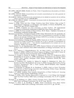
this illustrates that the Weibull approach is not the best approach to fit the wind power PDF.
For this location, the Gauss-Hermite and Kernel approaches have approximately the same
error. However, since the kernel estimates are produced using parameters which are
computed over the whole range, there is a tendancy and risk that the kernel approach will
be too weighted toward the lower (e.g., less significant, from an electrical production
standpoint) end of the spectrum, and therefore the Gauss-Hermite approach will yield
results which more accurately model the wind power density and the electrical production
potential.


Fig. 3. Actual and Modeled Wind Power Density at Boise City, Oklahoma. Values represent
model estimates of scaled wind power density. The Black curve Weibull distribution fit; the
Green curve is a Kernel estimator, and the Red curve is a Gauss-Hermite expansion fit.
3. Non-stationarities and impact of climate change
It is well-known that climate change can influence the radiation balance and therefore wind
patterns. Recent findings from the Intergovernmental Panel on Climate Change (IPCC, 2007)
have shown that greenhouse gas-induced climate change is likely to significantly alter
climate patterns in the future. One wind-industry relevant example is that climate change
global warming is expected to affect synoptic and regional weather patterns, which would
result in changes in wind speed and variability. Therefore, there is a need to examine
climate change scenarios to determine potential changes in wind speed, and thus wind

Wind Farm – Technical Regulations, Potential Estimation and Siting Assessment
170
power. Wind power facilities typically operate on the scale of decades, so understanding
any potential vulnerabilities related to climate variability is critical for siting such facilities.
An exhaustive review of the existing research on the projected impacts of climate change on
the wind industry can be found in Greene, et al. (2010). The purpose of this section is not to

reproduce that work, but to illustrate what the potential impacts might look like.
Thus, as an example of the specific impacts of climate change on a particular location, future
summer wind speed estimates at 10m were computed for Chicago, Illinois. The data used
represents estimates of daily wind speed. The dates of the model outputs were: 1990-1999,
and for the decades of the 2020s, 2040s, and 2090s This was accomplished by using the
Parallel Climate Model (PCM) model, and then downscaling the data. The PCM was
developed at the National Center for Atmospheric Research (NCAR), and is a coupled
model that provides state-of-the-art simulations of the Earth's past, present, and future
climate states (see Hayoe, et al., 2008a, 2008b). The projections for the future using the
AOGCM are based on the IPCC Special Report on Emission Scenarios (SRES, Nakićenović et
al., 2000) higher (A1FI) and lower (B1) emissions scenarios. These scenarios set the future
atmospheric carbon equivalent amounts based upon estimates of a range of variables that
could impact carbon emissions. These include estimates of future changes in population,
demographics, and technology, among others. The B1 scenario values are considered a
proxy for stabilizing atmospheric CO
2
concentrations at or above 550 ppm by 2100, and
atmospheric CO
2
equivalent concentrations for the higher A1FI scenario are approximately
1000 ppm (Nakićenović et al. 2000). These estimates do not explicitly model carbon
reduction policies, but are considered an approximate surrogates for carbon policy (B1), or a
“business as usual” option (A1F1).
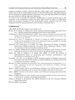
The results shown in Figure 4 illustrate the changes in average wind speed throughout the
spring and summer months (April – August), for the different decades listed above. Results
show a decrease for April -June of approximately 3-5% by the end of the century. There is a
slight increase for July and August. Overall for the summer, the total values are
approximately equal (decreases of 0-1%), but the changes in the seasonal patterns illustrate
the need for a more complete analysis in computing the climate change impact on wind
speed and wind power density. Also, potential carbon management policy implications

need to be considered. Figure 4 shows that there is a significant difference for the 2090s
between the policy and no-policy estimates. For example, the May values show a decrease of
5% for the no policy option, and increase of over 4% for the climate policy estimates. This
difference illustrates that for this location, a carbon management public policy would
dramatically increase the wind, and therefore the potential for increased electrical
production.
4. Summary and conclusions
This chapter has provided an overview of some key points associated with improved
understanding of wind farm siting. Specifically, the focus has been on two areas of
importance in this topic: 1) accurate wind resource assessment; and 2) potential
implications of climate change on the wind resource of the future.
For the first topic, there has been much research into the best way to model the wind speed
probability density function, as this is the core basis for estimation of the resource.
Traditionally, the industry standard has been to model the PDF using either a Weibull or
Rayleigh distribution. It has been pointed out that both of these approaches suffer severe
Advanced Wind Resource Characterization and
Stationarity Analysis for Improved Wind Farm Siting
171
limitations that call into question their effectiveness, and other approaches have been
suggested by a range of different authors. A review of the trends and current state of the
wind PDF modeling has been provided, illustrating a several new and potentially useful
approaches. However, many of these approaches have the same inherent flaws, in that the
efforts have been spent on modeling the wind speed PDF, when what the industry (e.g.,
utilities and electrical providers) are really interested in is an estimate of the amount of
electrical production. Thus, this analysis of the existing research has illuminated two areas
of potential improvement. First, continued improvements in the wind PDF modeling,
including, for example, adopting approaches from other disciplines, such as the Gauss-
Hermite approach illustrated above, are necessary to develop more accurate portrayals of
the resource. Second, geographers and climatological researchers need to more effectively
link their efforts to industry needs on trying to model, reproduce, and understand the

resource of interest to utilities (e.g., potential electrical production) rather than the more
simple and straightforward approach of analyzing the climatological variables (e.g., the
wind speed).


Fig. 4. Estimated Future Wind Speeds, Chicago. Values represent GCM-estimated wind
speeds.
Finally, previous research has shown a projected slight decrease in wind speeds in the
future, which would result in serious implications for wind farm siting. As shown in the
analysis performed here, in the United States, particularly for the wintertime, this is
theorized to be associated with a poleward shift of the mean thermal gradient as the earth
warms and results in a northward shift of the associated storm track patterns. It is
suggested that there will be pronounced regional and seasonal variability in the changes
that are currently underway. The wind industry has been growing exponentially over the
last decade, and is projected to expand and continue to play an ever-increasing role in
electrical production around the world. Improved understanding of the resource, and in any
inherent non-stationarities in the wind will help with transition to a sustainable energy
future.
3.50
3.70
3.90
4.10
4.30
4.50
4.70
4.90
5.10
5.30
April May June July August
Wind Speed (m/s)

Month
1990s
2020s
2040s

Wind Farm – Technical Regulations, Potential Estimation and Siting Assessment
172
5. Reference
Brock, F. V., Crawford, K. C., Elliott, R. L., Cuperus, G. W., Stadler, S., Johnson, H., and Eilts,
M. (1997). The Oklahoma Mesonet: A technical overview. Journal of Atmospheric and
Oceanic Technology , 12, pp. 5-19.
Celik, A. N., (2003a). Assessing the suitability of wind speed probability distribution
functions based on wind power density. Renewable Energy 28, pp.1563-1574.
Celik, A. N., (2003b). A statistical analysis of wind power density based on the Weibull and
Rayleigh models at the southern region of Turkey. Renewable Energy 29, pp.593-604.
Conradsen, K., Nielsen, L. B., and Prahm, L. P. (1984). Review of Weibull statistics for
estimation of wind speed distributions. Journal of Climate and Applied Meteorology
23, pp.1173-1183.
Garcia-Bustamante, E., Gonzalez-Rouco, J. F., Jimenez, P. A., Navarro, J. and Montavez, J.P.
(2008). The influence of the Weibull assumption in monthly wind energy
estimation. Wind Energy 11, pp.483-502.
Greene, J.S., M.L. Morrissey, and S. Johnson (2010). Wind Climatology, Climate Change, and
Wind energy, Geography Compass, 4/11, 1592-1605.
Hall, P., (1980). Estimating a density of the positive half line by the method of orthogonal
series. Annals of the Institute of Statistical Mathematics 32, pp.351-362.
Hayhoe, K., Cayan, D., Field, C. B., Frumhoff, E. P., Maurer, E. P., Miller, N. L., Moser, S. C.,
Schneider, S. H., Cahill, K. N., Cleland, E. E., Dale, L., Drapek, R., Hanemann, R.
M., Kalkstein, L. S., Lenihan, J., Lunch, C. K., Neilson, R. P., Sheridan, S. C., and
Verville, J. H., (2008). Emissions pathways, climate change, and impacts on
California. Proceeding of the National Academy of Sciences 101, pp.12422-12427.

Hayhoe, K., Wake, C., Anderson, B., Liang, X. L., Maurer, E., Zhu, J., Bradbury, J.,
DeGaetano, A., Stoner, A., and Wuebbles, D., (2008). Regional Climate Change
Projections for the Northeast USA. Mitigation and Adaption Strategies for Global Change.
DOI 10.1007/s11027-007-9133-2.
Hennessey, J. P, Jr., (1977). Some aspects of wind power statistics. Journal of Applied
Meteorology, 16, pp.63-70.
Intergovernmental Panel on Climate Change, IPCC, (2007). The Physical Science Basis, Fourth
Assessment Report.
Izenman, A. J., (1991). Recent developments in nonparametric density estimation. Journal of
the American Statististical Association, 86, pp.205-224.
Jaramillo, O. A., and Borja, M. A., (2004). Wind speed analysis in La Ventosa, Mexico: A
bimodal probability distribution case. Renewable Energy 29, pp.1613-1630.
Juban, J., Siebert, N., Kariniotakis, G. (2007). Probabilistic short-term wind power forecasting
for the optimal management of wind generation. Proceedings of PowerTech 2007
IEEE Conference, Lausanne, Switzerland.
Justus, C. G., (1978). Winds and wind system engineering. Franklin Institute Press,
Philadelphia, PA.
Justus, C.G., and Mikhail, Amir. (1976). Height variation of wind speed and wind
distribution statistics. Geophysical Research Letters 3, pp.261-264.
Justus, C. G., Hargraves, W. R., Mikhail, Amir, and Graber, Denise. (1978). Methods for
estimating wind speed frequency distributions. Journal of Applied Meteorology 17,
pp.350-353.
Koeppl, G. W., (1982). Putnam’s Power from the Wind. Von Nostrand, pp.470.
Advanced Wind Resource Characterization and
Stationarity Analysis for Improved Wind Farm Siting
173
Lackner, M. A., Rogers, A. L., Manwell, J. F., (2008). Uncertainty analysis in MCP-based
wind resource assessment and energy production estimation. J. Solar Energy Eng.
130, doi: 10.1115/1.2931499.
Liebscher, E., (1990). Hermite series estimators for probability densities. Metrika 37, pp.321-

343.
Li, M., and Li, X., (2005). MEP-type distribution function: A better alternative to Weibull
function for wind speed distributions. Renewable Energy 30, pp.1221-1240.
Luna, R. E. and Church, H. W. (1974) Estimation of Long-Term Concentrations Using a
Universal Wind Speed Distribution. Journal of Applied Meteorology 13, pp.910-916.
Monahan, A. H., (2006). The probability distribution of sea surface winds. Part II: Dataset
intercomparison and seasonal variability. Journal of Climate 19, pp.521-534.
Morrissey, M.L., Albers, A., J.S. Greene, and S.E Postawko (2010a), “An Isofactorial Change-
of-Scale Model for the Wind Speed Probability Density Function”, Journal of
Atmospheric and Oceanic Technology, 27(2): 257-273.
Morrissey,M.L., W.E. Cook, J.S. Greene (2010b), An Improved Method for Estimating the
Wind Power Density Function, Journal of Atmospheric and Oceanic Technology, 27(7):
1153-1164.
Najac, J. Boe, Julien and Terray, Laurent. (2009). A multi-model ensemble approach for
assessment of climate change impact on surface winds in France. Climate Dynamics
32, pp.615-634.
Pavia, E. G., and O’Brien, J. J. (1986). Weibull statistics of wind speed over the ocean. Journal
of Climate and Applied Meteorology 25, pp.1324-1332.
Pirazzoli, P. and Tomasin, A. (1990). Recent abatement of easterly winds in the northern
Adriatic. International Journal of Climatology 19, pp.1205-1219.
Ramirez, P. and Carta, J. A. (2005). Influence of the data sampling interval in the estimation
of the parameters of the Weibull wind speed probability density distribution: a case
study. Energy Conservation and Management 46. pp.2419-2438.
Rehman, Shafiqur and Al-Abbadi, Naif M. (2008). Wind shear coefficient, turbulence and
wind power potential assessment for Dhulom, Saudi Arabia. Renewable Energy
33. pp.2653-2660.
Sailor, D. J., Rosen, J. N., Hu, T., Li., X. (1999). A neural network approach to local
downscaling of GCM output for assessing wind power implications of climate
change. Renewable Energy 24. pp.235-43.
Schoof, J. T. and Pryor, S.C. (2003). Evaluation of the NCEP-NCAR Reanalysis in terms of

the synoptic-scale phenomena: A case study from the Midwestern USA.
International Journal of Climatology 23. pp.1725-1741.
Schwartz, M. and Elliott, D. (2006). Wind shear characteristics at central plains tall towers,
NREL/CP-500-40019.
Schwartz, S. C. (1967). Estimation of a probability density by an orthogonal series. Annual
Mathematical Statistics 38. pp1262-1265.
Segal, M., Pan, Z., Arritt, R. W., and Takle, E.S. (2001). On the potential change in wind
power over the US due to increases of atmospheric greenhouse gases. Renewable
Energy 24. pp.235-243.
Silverman, B. W. (1986). Density Estimation. London: Chapman and Hall.

Wind Farm – Technical Regulations, Potential Estimation and Siting Assessment
174
Stevens, M. J. M., Smulders, P. T. (1979). The estimation of the parameters of the Weibull
wind speed distribution for wind energy utilization purposes. Wind Energy 3.
pp.132-145.
Stewart, D. A., and Essenwanger, O. M. (1978). Frequency distribution of wind speed near
the surface. Journal of Applied Meteorology 17. pp.1633-1642.
Tuller, S. E. (2004). Measured wind speed trends on the west coast of Canada. International
Journal of Climatology 24. pp.1359-1374.
Tuller, S. E., and Brett, A. C. (1984). The characteristics of wind velocity that favor the fitting
of a Weibull distribution in wind speed analysis. Journal of Climate and Applied
Meteorology 23. pp.124-134.
Wackernagel, H. (2003). Multivariate Geostatstics. New York, NY: Springer.
0
Spatial Diversification of Wind Farms: System
Reliability and Private Incentives
Christopher M. Wo rley and Daniel T. Kaffine
Colorado School of Mines
USA

1. Introduction
A growing literature suggests that intermittency issues associated with wind power can be
reduced by spatially diversifying the location of wind farms. Locating wind farms at sites
with less correlation in wind speeds smooths aggregate electricity generation produced by
the multiple sites. However, technical studies focusing on optimal siting of wind farms to
reduce volatility of total wind power produced have failed to address the underlying private
incentives regarding spatial diversification by individual wind developers. This chapter
makes a simple point: Individual wind developers will in general seek out the windiest sites
for development, and as these locations are likely to be highly correlated in a given region, this
pattern of development will tend to amplify (rather than smooth) problems associated with
the variable nature of wind power. As such, private wind developers cannot be depended
upon to provide reliability benefits from spatial diversification in the absence of additional
incentives.
Wind power is growing rapidly in the United States and throughout the rest of the world.
As concerns about global climate change intensify, policymakers and power utilities look
to less carbon-intensive energy sources.
1
As a near-zero emission source of generation,
wind provides a mature alternative technology with some of the most competitive renewable
energy costs.
2
However, the potential for wind power to provide a substantial percentage
of world electricity is hindered by the stochastic nature of the wi nd resource. Due to
this intermittency, electricity from wind power cannot be dispatched like electricity from a
coal boiler or a natural gas turbine. The day-to-day and hour-to-hour variability of wind
power requires power utilities to maintain excess capacity of dispatchable electricity or face a
potential shortfall when wind speeds diminish.
The capacity credit of wind power—the amount of dirty capacity that can be removed from the
grid—is around 20% when wind power is initially added to the generation portfolio. In other
1

The precise level of emissions avoided by wind power is a topic of much debate, and likely varies
considerably with the existing generation mix, load levels, and other factors (Kaffine et al., 2011;
Novan, 2010). The intermittency issues addressed in this chapter are in fact related to emission
savings from wind power, as substantial variability in wind generation levels may require aggressive
(emissions-intensive) ramping of thermal generation for load balancing.
2
The Energy Information Administration Annual Energy Outlook 2011 (DOE/EIA-0383) gives
U.S. national averages for the levelized costs of energy for different energy sources, including
wind ($97.0/MWh), conventional coal ($94.8/MWh), solar PV ($210.7/MWh), and solar thermal
($311.8/MWh) under an assumed $15 per metric ton of CO2 emissions fee.
8
2 Will-be-set-by-IN-TECH
words, a wind farm with a nameplate capacity of 100 MW may only remove around 20 MW
of dirty capacity. Furthermore, each additional marginal megawatt of wind capacity installed
has a diminished ability to remove dirty generating capacity.
3
If the aggregate supply of wind
power were more reliable, then less backup generation capacity would be needed per MW of
wind capacity. Thus, improving the reliability of wind power reaching the grid may provide
economic benefits by allowing system operators and utilities to better schedule generation and
reduce backup generation, not to mention the environmental benefits of reducing reliance on
dirty g eneration.
Empirical work has shown that sites with high mean wind speed also have high variance in
wind speeds.
4
Given this, there are two ways that the variability of wind power produced
by multiple wind farms may be reduced. First, wind farms could be built on sites with
low variance. Unfortunately, wind developers have little incentive to build on sites with
low wind speed variance because those sites also tend to have low mean wind speeds. The
second method for reducing the variability of wind generation would be to diversify the

supply of wind power over sites with low spatial correlation (an algorithm for determining
the variance-minimizing locations for wind farms is presented in Choudhary et al. (2011)).
Just as a diversified investment portfolio has less risk than investing in a single asset, a
spatially-diversified portfolio of wind capacity could improve the reliability of wind power,
reduce the risks of outage, and increase the capacity credit of wind power.
Kempton et al. ( 2010) examined offshore wind resources along the length of the Eastern
Seaboard of the United States and found that wind speed correlations between sites dropped
to 0.25 at around 500 km, implying that wind farms spread far apart could reduce the volatility
of wind power reaching the electrical grid. Based on their simulation results, it may be socially
beneficial if wind developers would hedge the unreliability of wind power by developing
wind power at spatially disparate sites with less correlated wind speeds. Kempton et al. (2010)
note that such a system may prove to be difficult to develop because electricity generation
is largely a state-level concern, and it may be difficult to align the incentives of the many
states required for a system of interconnected wind farms along the Eastern Seaboard. In
the particular case of the Eastern Seaboard, achieving such a spatial diversification of wind
farms would require the input and cooperation of four electricity reliability councils, the
public utilities commissions of fifteen states, dozens of power companies, and many, many
individual wind developers.
In fact, the role of locational investment incentives may be even more important at the
individual firm level. Roughly 80% of wind farms are independent power producers (IPP),
which are not owned or operated by power utilities.
5
These wind developers search for windy
sites on which to build, and then negotiate a Power Purchase Agreement (PPA) with the utility
to lock in a fixed rate for electricity sales. These independent wind developers are motivated
purely by the private cost-benefit analysis of site development, so they hunt for “jackpot”
sites with the greatest return (typically the very windiest sites with correspondingly high
variance). Furthermore, wind farms in a region are likely to be closely co-located in space
because meteorological wind speeds are spatially correlated. As a result, individual wind
3

A technical report from the National Renewable Energy Laboratory summarizes capacity credit
estimates from around the U.S., which tend to fall in the 5-35% range (Milligan & Porter, 2008).
4
As such, one potential model for wind speeds is a Weibull or Rayleigh distribution. Beenstock (1995)
argues that a Rayleigh distribution is a useful assumption that is a good baseline approximation of the
true wind distribution.
5
This estimate comes from interviews with wind researchers and wind industry professionals.
176
Wind Farm – Technical Regulations, Potential Estimation and Siting Assessment
Spatial Diversification of Wind Farms: System Reliability and Private Incentives 3
developers are unlikely to ultimately build on sites that enhance the reliability of the total
supply of wind generation.
To illustrate the central point of this chapter, we first develop a simple theoretical model to
compare the optimal siting decisions of individual wind developers versus the optimal siting
decisions of system operators.
6
Given a 1-dimensional region with a concave distribution of
wind speeds, all individual wind developers will choose to build as close to the wind speed
maximum as possible. As such, wind speeds at these wind farms will be highly correlated and
thus aggregate wind generation will be highly volatile. In contrast, the system operator will
trade off the benefits of generating electricity at the windiest site for a more reliable supply of
wind power, spreading out wind farms farther from the location of the wind speed maximum.
To provide further economic intuition, we present a closed-form analytical solution for siting
decisions that can be generalized for up to n wind farms.
To highlight the divergence of incentives between decentralized wind developers and the
system operator, we develop a spatial optimization model, loosely calibrated to the plains of
eastern Colorado, whereby agents maximize profit by choosing a number of locations for wind
farms. In the case of individual, decentralized wind developers, each firm maximizes their
expected private returns by selecting the most profitable site for development, given wind

speed of known mean and variance. On the other hand, for the case of the system operator,
a single agent selects locations that maximize expected total returns from development and
includes costs associated with the reliability of aggregate wind power reaching the grid. The
model generates Rayleigh-distributed, correlated wind speeds for each site over a lengthy
time horizon. Importantly, wind speed correlation between sites declines over distance and
we allow for differing mean wind speeds for each site. Both the individual wind developers
and system operator select the location that maximizes their objective functions based on the
generated wind speeds.
There is a significant divergence between the optimal locational decisions of the individual
wind developers and the system operator. Individual wind developers choose to build on
the windiest sites, and as wind power produced at those sites is highly correlated, high
reliability costs are incurred. By contrast, the system operator internalizes the tradeoffs
between system reliability generated by diversified siting decisions and the profits associated
with the windiest sites, resulting in more spatially diverse locations being selected and an
improvement in reliability and total economic value. We note that providing the correct siting
incentives to individual wind developers will require those incentives to be conditioned on the
siting decisions by all other wind developers, and we finish this chapter with some concluding
remarks and suggestions for further work.
6
There are many parties that may receive benefits from wind reliability, including Independent
System Operators (ISO) responsible for load balancing, or rate payers who ultimately pay the cost
of maintaining backup generation, or public utilities who must ramp their thermal generation units
for load balancing. We use the ‘system operator’ as a catch-all for all such parties that receive
reliability benefits (in addition to economic returns from generation) and would therefore internalize
these benefits into their optimal decisions regarding wind farm location. We also recognize that the
economic incentives of real-world system operators may not precisely match those of the economic
agent that we have dubbed the ‘system operator’ in the analysis below. Ultimately we are interested in
comparing the siting decisions of individual wind developers interested in purely private profits versus
an economic agent with a more systemic outlook, concerned with system profits including benefits
and costs associated with system reliability. Determining the distribution of the costs and benefits of

reliability to the various parties is outside the scope of this study.
177
Spatial Diversification of Wind Farms: System Reliability and Private Incentives
4 Will-be-set-by-IN-TECH
2. Background
The electricity and wind engineering literatures have analyzed the role of wind farm locations
in electrical grid reliability as far back as Kahn (1979), who first notes that the variance of wind
power output decreases as the geographic distance between wind farms increases. Since then,
much work has been done to analyze this issue at many scales. Cassola et al. (2008) proposes a
procedure for minimizing wind power variance through optimal siting of wind farms over the
island of Corsica, which is slightly smaller than the State of Delaware. Millig an & Artig (1999)
analyzes potential wind sites in Minnesota, while Milligan & Factor (2000) analyzes sites in
Iowa and find that state-level diversification allows power utilities to reduce wind power
supply risk. Archer & Jacobson (2007) select nineteen sites in four mid- and southwestern
states (i.e., Kansas, Oklahoma, Texas, and New Mexico) and find results similar to those of
previous studies, mainly that reliability benefits increase with distance between wind farms
and reduced variability translates into fewer high and low wind events. Choudhary et al.
(2011) develop a variance-minimizing algorithm for wind farm additions in Oklahoma, and
find that the algorithm will select the site that is geographically most distant from existing
stations. Kempton et al. (2010) used five years of wind data from eleven offshore sites along
the Eastern Seaboard of the United States to test the reliability benefits of spatially diversifying
wind farms on a synoptic-scale, meaning that they test reliability with respect to differing
pressure patterns at distances of 1,000 km or greater. They find that such a system experienced
few periods of complete power outage or full capacity, and power levels changed slowly over
time.
While all of these studies show that there are reliability benefits of spatially diversified wind
farms (in terms o f reducing power variance), they fail to address how the incentives of
wind power developers may affect reliability. In fact, this issue has been overlooked by
the economics literature as well. To remedy this, we present a spatial optimization model
that simulates the differing locational incentives of wind power players. Spatial optimization

models have been broadly used for many types of land-use issues like optimal managing
of timber harvests with wildlife habitats (Hof & Joyce, 1992), the trade-offs of biodiversity
and land-use for economic returns (Kagan et al., 2008), and efficient utilization of urban
areas (Ligmann-Zielinska et al., 2008) among other types of problems. Before simulating the
decisions of wind power developers, we develop an analytical model to better understand the
intuition behind locational investment decisions.
3. Analytical model
How might we illustrate the differing incentives of private wind developers and a system
operator? We develop a simple analytical exercise that captures the spatial variation in wind
speeds and corresponding impacts on reliability.
7
Let wind speed v be distributed over
a 1-dimensional space
(−∞, ∞) given by the concave function v(x) where the maximum
windspeed v
max
is located at the origin x = 0. At a given site x, wind can be converted
into electricity (kWh) as represented by the function W
(v(x)) (where W
v
> 0). Each of two
individual wind developers will chose their privately optimal wind farm location (x
1
and x
2
)
that maximizes this objective:
max
x
i

π = pW(v(x
i
)) − F ∀i = 1, 2 (1)
7
In the spirit of using the simplest possible model to make an analytical point, much of the real-world
complexity of siting decisions have been stripped out.
178
Wind Farm – Technical Regulations, Potential Estimation and Siting Assessment
Spatial Diversification of Wind Farms: System Reliability and Private Incentives 5
where p is the per-unit price of electricity ($/kWh) and F is the fixed cost ($) of operating the
wind farm over the time horizon. The first-order conditions for building wind farms x
1
and
x
2
are given as:
π
x
i
= p
dW
dv
dv
dx
i
= 0 ∀i = 1, 2 (2)
Because v
(0)=v
max
, the location that maximizes profit for both wind developers exists at

the maximum of the wind speed distribution, such that x
∗
i
= 0, ∀i = 1, 2. Thus, when the
wind developers choose wind farm locations based on their private incentives, both wind
farms will be built as close as possible to the point with the highest mean wind speed. Due to
their proximity, wind speeds at these sites will be highly correlated, resulting in a supply of
wind power that is less reliable than had the two sites been located farther apart. Thus, any
benefits from spatial diversification are not realized under this setting where individual wind
developers select locations for wind development.
By contrast, the system operator internalizes the reliability benefits of spatial diversification
when locating wind farms. These reliability benefits will be simply expressed by the function
r
(d) (where r
d
> 0), such that the distance between wind farms is given as d = x
2
− x
1
.The
system operator’s optimization problem is given as the joint maximization of profits from
locating two wind farms plus reliability benefits from spatial diversification:
max
x
1
,x
2
π =
[
pW(v(x

1
)) − F
]
+
[
pW(v(x
2
)) − F
]
+
r( d) (3)
Given this objective, the first-order conditions are as follows:
π
x
1
= p
dW
dv
dv
dx
1
− r

(d)=0
π
x
2
= p
dW
dv

dv
dx
2
+ r

(d)=0
(4)
Given positive benefits of spatial diversification (r
d
> 0) and comparing against the
decentralized first-order conditions in equation 2, the system operator will choose to build on
either side of x
= 0(wherev(x) < v
max
). Relative to the case of individual wind developers,
the system operator will spread the wind farms farther apart (x
2
− x
1
> 0) as long as there are
positive marginal benefits from spatial diversification, r
d
> 0. While wind speeds are slower
and less power is produced at locations away from the location corresponding to v
max
,the
system operator offsets those power losses with the gains from a more reliable supply of wind
power.
These results can be generalized to the case of multiple wind farms. Individual wind
developers will choose to build all wind farms as close to v

max
as possible (x
∗
i
= 0, ∀i =
1, ,n). On the other hand, the system operator realizes reliability benefits depending on
the pairwise distances between wind farms, r
(d
ij
).
8
The system operator’s objective function
when choosing to develop three sites is given as the following:
8
More formal and realistic treatments of how reliability benefits might enter the system operator’s
objective function are certainly possible, though the basic intuition outlined below will still hold. For
simplicity, we will assume r

( d
ij
)=r

( d).
179
Spatial Diversification of Wind Farms: System Reliability and Private Incentives
6 Will-be-set-by-IN-TECH
max
x
1
,x

2
,x
3
π =
[
pW(v(x
1
)) − F
]
+
[
pW(v(x
2
)) − F
]
+
[
pW(v(x
3
)) − F
]
+
r(x
3
− x
2
)+r(x
3
− x
1

)+r(x
2
− x
1
)
(5)
Given this objective, the first-order conditions are given as:
π
x
1
= p
dW
dv
dv
dx
1
− 2r

(d)=0, π
x
2
= p
dW
dv
dv
dx
2
= 0, π
x
3

= p
dW
dv
dv
dx
3
+ 2r

(d)=0(6)
where the system operator locates one wind farm at the origin, and the remaining two wind
farms on either side of the origin.
A closed-form solution of the optimal development locations cannot be obtained without
some assumptions on the parametric forms of the spatial distribution of wind, wind power
production function, and reliability benefits of spatial separation between sites. Supposing
v
(x)=v
max
− bx
2
, W(v)=γv,andr

(d)=
¯
r we arrive at the system operator solution for the
two wind farm case:
9
x
∗
1
= −

¯
r
2pγb
, x
∗
2
=
¯
r
2pγb
(7)
and the three wind farm case:
x
∗
1
= −
¯
r
pγb
, x
∗
2
= 0, x
∗
3
=
¯
r
pγb
(8)

These closed-form solutions yield some intuitive comparative statics that illustrate the
tradeoffs that the s ystem operator faces. As the benefits from spatial diversification,
¯
r,
increase, the wind farms will be located further away from v
max
. By contrast, as the price
of electricity p increases, the system operator will value the profitable generation associated
with high wind speeds near v
max
relative to the reliability benefits. As a result, they will
build closer to v
max
. I n fact, an increase in any parameter in the denominator will shift the
optimal wind farm sites for the system operator closer to x
= 0. The parameter b captures
the curvature of the spatial distribution of wind speed. As this parameter increases, the
curvature of the wind speed distribution becomes steeper, further reducing the wind speed
at sites away from the origin and pushing development towards x
= 0andv
max
. Finally, the
parameter γ describes the efficiency of the wind turbines for producing electricity. When γ
increases, turbines become more efficient at producing power, and the reliability benefits of
spatial diversification become less valuable than building closer to the higher wind speeds
located at x
= 0.
These results can be extended to the case of n wind farms as given in table 1. In short, for an
even number of wind farms, the system operator will build matching wind farms equidistant
on either side of x

= 0. For an odd number of wind farms, the system operator will build one
wind farm on x
= 0, and build matching pairs of wind farms further and further away from
v
max
. By contrast, the individual wind developers will build as close to x = 0 as physically
possible.
9
As noted in Beenstock (1995), electricity is generated as a cubic function of the wind speed. While the
linear function W
( v)=γv fails to capture real-world characteristics of wind, this assumption allows
us to find a closed-form solution.
180
Wind Farm – Technical Regulations, Potential Estimation and Siting Assessment
Spatial Diversification of Wind Farms: System Reliability and Private Incentives 7
Numberofwindfarms 12345 n
Individual developer locations
Windfarm1 n 0 0 0 0 0 0
System operator locations
Wind farm 1 0
−
¯
r
2pγb
−
¯
r
pγb
−
3

¯
r
2pγb
−
2
¯
r
pγb
−
(n−1)
¯
r
2pγb
Wind farm 2 - +
¯
r
2pγb
0 −
¯
r
2pγb
−
¯
r
pγb
−
(n−3)
¯
r
2pγb

Wind farm 3 - - +
¯
r
pγb
+
¯
r
2pγb
0 −
(n−5)
¯
r
2pγb
Wind farm 4 - - - +
3
¯
r
2pγb
+
¯
r
pγb

Windfarm5
+
2
¯
r
pγb



Wind farm n
− 1 +
(n−3)
¯
r
2pγb
Wind farm n +
(n−1)
¯
r
2pγb
Table 1. Optimal wind farm location decisions for individual wind developer and the system
operator
This analytical model is a very simplified version of the real-world spatial incentives of
wind development. In the next section, we design a numerical simulation model that is
multidimensional, has stochastic and spatially-correlated wind speeds, and features a more
realistic power curve. Calibrating the simulation model to real-world parameters allows us to
capture the relative scale of the trade-offs involved.
4. Simulation model
To highlight the differing incentives of individual wind developers and the system operator,
we next develop a spatial optimization model. As in the previous section, we will be
comparing the optimal siting decisions of individual wind developers with those of the
system operator. The physical space is a 3-x-3 grid of n
= 9 potential sites for development
with wind speeds of known mean and variance. We generate Rayleigh-distributed,
spatially-correlated random wind speeds for each site over 1,000 days (with one random draw
per day), allowing differing mean wind speeds for each site.
10
The windiest sites are located

near each other (see figure 1(a)), and the wind speed correlation between sites declines with
the pairwise distance between sites (see figure 1(b)).
We very loosely calibrate the model to the northeastern plains region of the State of Colorado,
a windy part of the state with some wind development. Each of the sites in figure 1(a) would
be 100 km on each side, meaning that the nine sites would roughly cover an area from the
northeastern corner of the state to Colorado Springs (roughly located in the center of the
state). The U.S. Department of Energy provides state level wind maps, showing that Colorado
has windy locations along the eastern border with Nebraska, Kansas, and Oklahoma.
11
The
general pattern of wind speeds from these state level wind maps provide the basis for the
mean wi nd speed distribution across the nine sites in the model. Site 9 is the windiest
10
The procedure for generating Rayleigh-distributed, spatially correlated wind speeds is adapted from
Natarajan et al. (2000) and Tran et al. (2005)
11
The DOE Office of Energy Efficiency & Renewable Energy maintains a
website that provides maps of wind resource potential at 80 meter heights
( Accessed 2/18/2011).
181
Spatial Diversification of Wind Farms: System Reliability and Private Incentives
8 Will-be-set-by-IN-TECH
Site 7 Site 8 Site 9
Site 4 Site 5 Site 6
Site 1 Site 2 Site 3
6.50 6.75 7.00
6.25 6.50 6.75
6.00 6.25 6.50
(a) Mean wind speed (m/s)
d=1.00

=0.50
d=1.41
=0.40
d=2.00
=0.30
d=2.24
=0.20
d=2.83
=0.10
(b) Correlation coefficient ρ based on distance d
between sites
Fig. 1. Mean wind speed and pairwise correlations for 3x3 scenarios
site with wind speeds decreasing with distance from Site 9, meaning that Site 1 is the least
windy location. We generate wind speed correlations between sites that decay over distance
in the spirit of Kempton et al. (2010, Fig. 2). We stress that the quantitative results below
are primarily illustrative, with the primary insights of the simulation model arising from the
qualitative comparison of the siting decisions made by individual wind developers versus the
system operator.
4.1 Individual wind developer model
We begin by simulating two wind farm developers each choosing the site (1, ,n)that
maximizes their expected profit over the time horizon, T
= 1000. As in the analytical model
developed above, individual wind developers are only interested in the private economic
return from developing a given site for wind power. Each wind developer i has an identical
objective function:
max
X
i
π =
n

∑
i=1
T
∑
t=1
pk
it
X
i
−
n
∑
i=1
c
i
X
i
(9)
The binary choice variable, X
i
, equals 1 when the developer builds a wind farm on site i
and 0 otherwise, and a developer cannot build on a site that has already been built upon
by the other developer.
12
The parameter p is the price of electricity, which we assume to be
$0.10.
13
We assume that the fixed costs of operating a wind farm, c
i
, are equal at all sites,

which we estimate to be $557,160 over the 1,000 day time horizon.
14
The variable k
it
is the
12
The size of the wind farm (i.e., the number of turbines) arbitrarily affects the model, only scaling the
magnitude of each scenario’s profit and power produced. While one could simulate 10, 20, or 100
turbines, we simplify the model by assuming that each wind farm consists of one turbine.
13
A value close in scale to estimates in the Energy Information Administration Annual Electric Power
Industry Report (Form EIA-861).
14
This is based on estimates from Elkinton et al. (2006) that annualized fixed costs plus yearly variable
costs of 3.7 cents/kWh - 5.5 cents/kWh. We choose levelized production costs of 6.0 cents/kWh. Given
that the mean power produced at Site 9 at any given time is 9,286 kW, we arrive at a fixed cost of
$557,160 over the 1,000 day time horizon. This is held constant over all sites even though the levelized
production costs may differ for sites with slower mean wind speeds.
182
Wind Farm – Technical Regulations, Potential Estimation and Siting Assessment
Spatial Diversification of Wind Farms: System Reliability and Private Incentives 9
generation (in kWh) at site i in time period t . This is calculated from the spatially-correlated
Rayleigh-distributed randomly drawn wind speeds v
it
via the following power function:
k
it
=
⎧
⎪

⎪
⎨
⎪
⎪
⎩
0if0
≤ v
it
< 4
λ
· v
3
it
if 4 ≤ v
it
< 11
λ
· (11)
3
if 11 ≤ v
it
≤ 25
0ifv
it
> 25
(10)
The parameter λ is the power proportionality constant that converts wind speeds in m/s to
electricity generation in kWh.
15
Wind turbines are able to generate electricity only over certain

wind speeds. No electricity can be generated for wind speeds below 4 m/s as the wind is too
slow. For wind speeds above 4 m/s, electricity is proportional to the cube of wind speed,
topping out at 11 m/s. Constant generation is produced for windspeeds between 11 - 25 m/s,
and for speeds above 25 m/s, turbines are shut down for fear of damage.
Each developer is constrained to build on only one site:
n
∑
i=1
X
i
≤ 1 (11)
Thus, given a draw of 1,000 Rayleigh-distributed, spatially correlated wind speeds v
it
at each
site i for each period t, each wind developer selects the site for development that maximizes
private profits.
4.2 System operator model
The system operator chooses the location of two wind farms by balancing the high revenues
associated with concentrating development at windier sites with the reliability cost of spatial
diversification. The objective function looks similar to that of individual wind developers
except for the addition of the reliability cost variable, R
t
, in each time period t. The system
operator incurs a nonnegative reliability cost (in dollars) for each time period when the system
supply of wind power is less than the expected level.
16
The system operator’s objective
function is as follows:
max
X

1
,X
2
π =
n
∑
i=1
T
∑
t=1
pk
it
X
i
−
n
∑
i=1
c
i
X
i
−
T
∑
t=1
R
t
(12)
The system operator is constrained to build on two sites:

n
∑
i=1
X
i
≤ 2 (13)
15
For an assumed 1.5 MW wind turbine rated at 11 m/s, the power proportionality constant is equal to
1128 (found by simply dividing 1,500,000 by 11
3
)
16
Thus, reliability costs are incurred when the sum of wind power from the two wind farms falls below
expected levels. It should be noted that we are only considering the reliability costs associated with
a shortfall in wind generation. However, it may also be the case that a temporary overabundance of
wind generation can also be problematic from the perspective of the system operator. For example,
large amounts of wind power reaching the grid may require sudden and costly curtailment of other
generation sources, which then have to be ramped back online when wind power diminishes. Including
such considerations would further sharpen the contrast between the incentives of individual wind
developers and the reliability-internalizing system operator.
183
Spatial Diversification of Wind Farms: System Reliability and Private Incentives
10 Will-be-set-by-IN-TECH
The system operator model has two additional constraints that define and ensure
nonnegativity of the reliability cost. This first constraint calculates the value of the reliability
cost, which we conceptualize as the cost of maintaining back up generating capacity or
purchasing electricity on the wholesale market when a wind farm’s generation k
it
does not
meet the mean generation level

k
i
.
17
The parameter z is the per-unit reliability cost, which we
set at $0.10.
18
The difference
∑
n
i
=1
(k
i
− k
it
)X
i
is the system power shortage in period t.The
parameter M is an arbitrarily large number and the binary variable β
t
is equal to 1 when there
is a system shortage of wind power and equal to 0 otherwise.
19
R
t
≥ z ·
n
∑
i=1

(k
i
− k
it
)X
i
− M(1 − β
t
) ∀t (14)
This second constraint forces the reliability cost to be zero when k
it
> k
i
.
n
∑
i=1
k
it
· X
i
≥
n
∑
i=1
k
i
· X
i
− β

t
· M ∀t (15)
The system operator problem is solved by jointly selecting the two best sites, accounting for
the benefits from spatial diversification.
4.3 Results
Before discussing the optimization results, we begin with a cursory examination of wind
power produced from randomly generated, Rayleigh-distributed, spatially correlated wind
speeds at sites with varying levels of spatial diversification. Figure 2 compares the capacity
factor of two wind farms over a horizon of 100 time periods for three different groupings of
the two wind farms.
20
We wish to compare the variability in power supplied when there are
two wind farms located on Site 3, one on Site 3 and one on Site 5, and one on Site 3 and one on
Site 7. Visual comparison in figure 2 of the joint capacity factor across groupings is somewhat
difficult, but there are fewer dramatic peaks when wind farms are spatially diversified in
figure 2(c) compared to when wind farms are co-located in figure 2(a). This suggests that the
volatility of wind supply from wind farms on Sites 3 and 7 is less than that of two wind farms
co-located on Site 3.
As noted in figure 1(b), these three sites have the same mean wind speed and variance, but
when wind farms are located at less spatially correlated sites, there is a reduction in the total
variance o f total power produced. For two wind farms co-located on Site 3, the sample
variance in capacity factor is 0.093. The sample variance decreases as the wind farms are
located farther apart. For wind farms on Sites 3 and 5, the sample variance is 0.076, and for
Sites 3 and 7, the sample variance is 0.061.
17
As noted previously, this is a simplification of the cost imposed on the utility when they have an
unreliable source of power, but it allows for a tractable solution with easily interpretable results.
18
We believe this to be a reasonable cost, as this might be the price that a utility pays for electricity on the
spot market or for natural gas backup generation.

19
The variable β and the parameter M are used in these constraints to ensure nonnegativity of the
reliability cost as is consistent with “Big-M” formulations.
20
Capacity factor is the percentage of nameplate capacity that a turbine produces at a given point in
time. For example, a 2 MW turbine operating with a capacity factor of 0.6 would produce 1.2 MW of
electricity.
184
Wind Farm – Technical Regulations, Potential Estimation and Siting Assessment
Spatial Diversification of Wind Farms: System Reliability and Private Incentives 11
Capacity Factor
(a) Two wind farms on Site 3
Capacity Factor
(b) W ind farms on Sites 3 and 5
Capacity Factor
(c) Wind farms on Sites 3 and 7
Fig. 2. Capacity factor of two wind farms
As theory suggests, spatial diversification reduces the volatility of the supply of wind power.
But how do agents respond to these diversification incentives? We run the optimization
model over the 1,000 day time h orizon with daily random wind speed draws for each site and
determine the optimal siting decisions of individual wind developers and a system operator.
However, the locations chosen represents the optimum for a specific set of 1,000 day random
draws. To get a better sense of the incentives as play, the model itself is simulated over 1,000
runs, with the optimal decisions for each run recorded and reported in distribution form
below.
As discussed in the analytical model, because individual wind developers do not receive any
benefits from spatial diversification, they will look to develop on the sites with the highest
expected electricity production (and therefore profits). The simulated optimal siting decisions
for the individual wind developers are shown in figure 3.
As the model is run 1,000 times, the results in (figure 3(a)) give the number of times out of 1,000

that site was selected for a wind farm by the individual wind developers. As suggested in the
analytical model, most wind development is clustered around the site with the highest mean
wind speed, Site 9. Sites 6 and 8 are the next windiest sites and are selected the next greatest
185
Spatial Diversification of Wind Farms: System Reliability and Private Incentives
12 Will-be-set-by-IN-TECH
853410121
16 65 409
112131
(a) Wind farm locations
Distance
Frequency
(b) Histogram of pairwise distances between
wind farms
Fig. 3. Individual wind developers location results
number of times. The pairwise distance between wind farms is calculated for each run, and, as
expected, most wind farms built by individual developers are built a single unit apart (figure
3(b)). Thus, individual wind developers are typically selecting the jackpot outcome in the
northeast corner of the grid and are not spatially diversifying wind farms.
In contrast to individual wind developers, the system operator benefits from higher wind
speeds but also incurs the costs of any demand shortfall should the wind not blow. The system
operator maximizes profit by jointly considering windy sites and the benefits from a more
reliable wind portfolio. We again present the results of the simulation model as a distribution
of optimal siting decisions and a histogram of the pairwise distance between wind farms for
each run (figure 4).
In contrast to the locations chosen by individual wind developers, the system operator
chooses to develop sites all around the map (figure 4(a)). In particular, locations near the
center of the grid (Site 5) are eschewed in favor of more spatially disparate sites due to the
reliability benefits from less correlated wind speeds. The histogram makes this point even
more clear (figure 4(b)), as the most common pairwise distance between sites is 2.24 units

(Sites 6 and 7 for example - the equivalent of a ‘knight-move’ in chess), followed by the
maximum distance of 2.83 units (Sites 3 and 7 or Sites 1 and 9, corresponding to the corners).
The system operator is willing to choose sites with lower mean wind speed due to the benefits
of a reliable supply of wind power.
In addition to the differences between the optimal siting d ecisions of i ndividual wind
developers and the system operator, system profits and total power produced differ as
well.
21
Table 2 lists total power and system profit results for the individual wind developer
and system operator scenarios averaged over the 1,000 simulated runs. Noting again that
the quantitative values are subject to the various parameter assumptions, we focus on the
21
We define system profit as total revenue - fixed costs - reliability cost, ignoring which party actually
receives the revenues and costs in each scenario. The total power shortage is defined as the sum of
power shortages at both wind farm over all time periods.
186
Wind Farm – Technical Regulations, Potential Estimation and Siting Assessment
Spatial Diversification of Wind Farms: System Reliability and Private Incentives 13
324174351
171 63 181
343179214
(a) Wind farm locations
Distance
Frequency
(b) Histogram of pairwise distances between
wind farms
Fig. 4. System operator location results
relative differences between the two scenarios. Most notably, the reliability cost is reduced
by 27% under the system operator scenario as compared to the individual wind developer
scenario, reflecting the less volatile wind supply at sites chosen by the system o perator.

Correspondingly, the locations selected by the system operator reduce total power shortage
by 15% relative to the sites selected by individual wind developers. As the system operator
internalizes reliability costs when selecting sites, total system profit increases by 8% under
the system operator scenario relative to the individual wind developer scenario. However,
by trading off windier sites for a more reliable supply of power, the total power produced
decreases under the system operator, but only by about 2%.
System Reliability Total Power Total Power
Scenario Profit ($) Cost ($) Produced (kWh) Shortage (kWh)
Individual wind developers 942,542 481,740 25,385,700 6,278,120
System operator 1,015,220 350,656 24,801,600 5,344,600
Table 2. System profits, reliability costs and power results
These results s how that while individual wind developers are privately be tter off when
they choose the windiest sites for development, they pass along large reliability costs as
an externality that is directly borne by the system operator (or other economic agents). By
contrast, the system operator trades off the benefits of high wind speed sites for a reliable
portfolio of sites, resulting in an increase in system profit and only a minor decrease in total
power produced.
22
22
To the extent that wind power offsets emissions-intensive forms of generation, changes in total power
produced may also have economic efficiency implications. However, in this particular case, the extra
power production under the individual wind developer scenario comes at the substantial cost of 12
cents of system profit per additional kWh of generation.
187
Spatial Diversification of Wind Farms: System Reliability and Private Incentives
14 Will-be-set-by-IN-TECH
5. Discussion
We conclude with a discussion of how incentives may be structured to encourage individual
wind developers to appropriately internalize reliability costs. We also discuss how additional
factors omitted from the above analysis might affect spatial diversification and end with some

concluding remarks and directions for future work.
5.1 Incentives for individual wind developers to spatially diversify
While spatially-diversified wind farms may generate reliability benefits, if individual wind
developers do not receive those benefits, their locational decisions for development will not
internalize these benefits and the total supply of wind power will be less reliable. Creating
incentives for individual wind d evelopers to internalize their reliability effects and spatially
diversify would likely take two forms: price premiums or penalties. First, site-specific
deterministic prices could be built into PPA’s, whereby a relative price premium would be
attached to sites that improve reliability. Second, s ome form of deterministic or stochastic
penalty could be levied conditional on the generation level produced by individual wind
developers.
Whatever form these incentives take, they must be set conditionally with respect to the
locations and spatial correlations of all other wind farms. So for a deterministic site-specific
pricing system, the price paid for development at a given site would have to appropriately
internalize the marginal impact of an additional wind farm on system reliability. For a penalty
system, the penalty applied to an individual farm would need to be tied to systemic shortfalls
in generation from all wind farms to generate the correct incentives to spatially diversify.
23
By
contrast, a flat wind integration charge, such as the 0.6 cents per kWh charge imposed by the
Bonneville Power Authority (BPA) (Choudhary et al., 2011), will not provide any incentive
for an individual wind farm to spatially diversify and choose a location that improves system
reliability.
24
5.2 Additional factors affecting locational decisions
The preceding analysis explored the optimal siting incentives of individual wind developers
versus the system operator. Locational incentives were driven by differences in mean wind
speeds and spatial correlations between sites. However, factors such as access to transmission
lines and interactions between wind farms also play a role in siting decisions. In particular,
transmissions costs and constraints are likely to generate additional incentives for spatial

clustering of wind farms as individual wind farms minimize any private costs incurred with
transmission. By contrast, wake effects between wind farms (Kaffine & Worley, 2010) may
lead to some spatial diversification by individual wind farms, however the scale of wake
23
See Worley (2011) for a further exploration of different penalty structures and the corresponding
impacts on locational decisions and system profit, reliability and power. In particular, Worle y (2011)
finds that a penalty leveled on individual wind developers when aggregate wind generation levels
fall below a threshold power level will provide individual wind developers the correct incentives to
spatially diversify like the system operator. Despite the theoretical appeal of a penalty system that
generates individual penalties based on system performance, such a penalty scheme may be difficult
to implement. A penalty scheme of this nature is similar to ambient pollution taxes (Segerson, 1988)
which have appealing theoretical properties but have not been frequently employed.
24
Note that we are not commenting on the wisdom of such a charge as there are obviously other reasons
for imposing such charges (such as cost-recovery). We simply mention it as an example of a penalty
scheme that would not provide incentives for spatial diversification.
188
Wind Farm – Technical Regulations, Potential Estimation and Siting Assessment