Satellite Monitoring and Mathematical Modelling of
Deep Runoff Turbulent Jets in Coastal Water Areas

169

Fig. 6. Propagation areas for anomalies caused by the deep outfall in Mamala Bay
(Hawaii)detected in optical (a) and radar (b) satellite images for different days under
various hydrometeorological conditions

5.5 Anomalies of hydrooptical characteristics detected using high resolution satellite
imagery and sea truth data
The processing of high resolution (2…4 m) multispectral images was carried out using the
characteristics of relative signal variety in red (R), green (G), and blue (B) spectral bands of 60 –
80 nm width. The processing technique used the following basic procedures (Bondur, 2004;
Bondur, Zubkov, 2005): synthesizing the colour image from separate bands (RGB-synthesis);
interpreting imagery to mark out clouds, ships and their traces, land, and unclouded marine
surface; selecting fragments of the full scene of an image for the area of interest for further
processing; filtering; decorrelation stretch to remove correlation of spectral bands; parametric
and non-parametric classification; combination of classes; colour coding.
To correct brightness image distortions caused non-uniform sensitivity of the CCD camera,
additional procedures consisting in removing brightness transversal trend within each
fragment; and brightness band interleveling based on statistic parameter use.
To verify the results of multispectral satellite imagery processing in the studied area, sea
truth measurements were carried out using AC-9 hydrooptical equipment and various
hydrophysical equipment at the moments of time close to satellite imaging time (Gibson et
al., 2006; Bondur et al., 2006a; 2007)/ The gauge was deployed from the
Klaus Wyrtki ship
down to a depth of 150 m. Values of absorption factor and attenuation were measured using
AC-9 equipment at nine wavelengths (in 412 to 715 nm spectral band) at each station (B6)
located in the area of the outfall. Vertical profiles of these values were created for each
station (Bondur et al., 2006a). To process AC-9 data we used the method based on the

Haltrin-Kopelevich linear bio optical model (Kopelevich, 1983; Haltrin & Kattawar, 1993).
Waste Water - Evaluation and Management

170
Fig. 7 presents the examples of multispectral QuickBird image processing (September 14,
2003; 11:16 LT imaging time). In this Fig. we can see: image fragment (16.5 х 16.5 km
2
)
synthesized from RGB bands of the original image (a); interim processing result consisting
in obtaining pixel-by-pixel band signal ratios blue/green, in a convolution with mask and
classification with further smoothing (b); result of combination of classes of similar
brightness with colour palette changing (c); re-combination of classes, detection and
outlining of anomalies (d).
The analysis of processing result shows that in the area of the Sand Island outfall diffuser
(right part of Fig. 7,d) anomaly of subsurface ocean layer hydro-optical characteristics is
evident.
Maximal size of this anomaly is about 6 km. Inside of this area more contrast extensive
anomaly (~ 3.5 km length) oriented in south direction, is detected. Another distinct surface
anomaly caused by oil spill due to leakage from a tanker during pumping to onshore
reservoirs is evident. Rather small anomaly of hydro-optical characteristics caused by
another outfall (Honouliuli) in Mamala Bay is seen on the left (see Fig. 7,d). Effectiveness of
the applied processing technology is confirmed by the fact that on original images
anomalies caused by the outfall are not seen.
Similar results were obtained after processing other multispectral satellite imagery as well
as multispectral data (Bondur, 2004; Bondur, Zubkov, 2005; Bondur et al., 2006a).


Fig. 7. Example of QuickBird multispectral image processing. a) original synthesized
images; b) processed fragment; c) classification with smoothing by a window; d)
combination of classes; e) final result

Satellite Monitoring and Mathematical Modelling of
Deep Runoff Turbulent Jets in Coastal Water Areas

171
For the comparison with satellite imagery processing results, absorption and attenuation
factors were used which had been obtained from AC-9 data at the wavelength of λ=0.488
μm, where sunlight absorption near the Hawaii was close to the minimum (Erlov, 1980).
Also, AC-9 spectral band coincided with the centre of QuickBird blue band.


Fig. 8. Comparison of the anomaly detected using QuickBird multispectral imagery
(September 3, 2004) (a) with 2D cross-sections of absorption at 0.488 μm wavelength (b);
chlorophyll C (c) and large particles (d) concentrations based on AC-9 data. ○ – Secchi disk
max visibility (b-d)
Fig. 8.a presents the outlined area of hydrooptical parameter anomaly detected using the
multispectral QuickBird image of September 3, 2004 near the deep outfall and ship trajectory
with indicated points where hydrooptical measurements had been carried out. Fig. 8 shows
2D distributions of absorption at λ = 0.488 μm (b), as well as chlorophyll C (c) and large
particle (d) concentrations based on AC-9 data.
The results obtained by Secchi disks have shown than at B6-3 and B6-5 Stations (near the
diffuser) maximum visibility was 48-51 m, while at B6-7 Station (far from the diffuser) it was
55.5 m. It is evident, that at B6-3 and B6-5 Station visibility decreased because of high
concentrations of various substances (organic, suspended particles, end etc.) contained in
wastewaters.
The processing analysis have shown the high level of coincidence both of western and
eastern anomaly boundaries detected using the satellite multispectral images with the
anomaly detected using hydrooptical data. The divergence of the results is 100 – 200 m.
Similar results were obtained during multispectral and hyperspectral satellite data
(HYPERION). Max anomaly size was 5 – 20 km (Bondur, 2004); Bondur & Zubkov, 2005;
Bondur et al., 2006a).

Waste Water - Evaluation and Management

172
Thus, the comprehensive analysis of the collected data have allowed us to interpret
unambiguously the processing results for multispectral imagery obtained during the
monitoring of anthropogenic impacts on the water environment.
6. Modelling the propagation of turbulent deep plumes
6.1 The model employed
A mathematical model described in (Bondur, Grebenyuk, 2001; Bondur et al., 2006b; 2009b)
has been used to study the propagation features of turbulent jets of contaminated waters
discharged into Mamala Bay. The jet propagation is described with a system of seven
ordinary differential nonlinear equations that characterize the balance of the horizontal and
vertical components of the momentum, the heat consumption, the salinity, and the jet
coordinates with the system being supplemented with the equation of the state of the sea
water. These equations have been obtained by integrating the equations of the motion,
continuity, and heat and salt balance under the assumption of scaling of the distributions of
the velocity, temperature and salinity in the cross section of the jet (Bondur et al., 2006b).
When deriving the equations, we considered a turbulent jet that was injected at the depth
z
into the aquatic medium at angle of Θ
0
to the sea line in the xz plain. The medium was
assumed to be incompressible and quiescent, and its density
ρ
a
(z) was depth dependent with
dρ
a
/dz < 0, which means the stable stratification of the medium (Bondur et al., 2006b).
The equation system looked as follows (Bondur et al., 2006b; 2009b):


2
()2=
d
ub ub
ds
α
, (9)

22
(cos)0
Θ
=
d
ub
ds
, (10)

22 22
0
0
(sin)2
−
Θ=
a
d
ub g b
ds
ρ
ρ

λ
ρ
, (11)

2
22
2
1
[( )]
+
−=
a
a
dT
d
ub T T b u
ds ds
λ
λ
, (12)

2
22
2
1
[( )]
+
−=
a
a

dS
d
ub S S b u
ds ds
λ
λ
, (13)

cos
=
Θ
dx
ds
,
sin
=
Θ
dz
ds
(14)

(,)= TS
ρρ
(15)
where T
a
(s) and S
a
(s) are the temperature and salinity of the medium, T(s) and S(s) are the
temperature and salinity of the jet; α = 0.057 is the entrainment coefficient; b = b(s) is the

characteristic half-width of the jet, and 1 = 1.16 is a constant; s is the coordinate along the jet
axis, r is the radial coordinate, u(s) and ρ(s) are the jet's axial velocity and density, ρ
0
= ρ
a
(0)
is the reference density.
Satellite Monitoring and Mathematical Modelling of
Deep Runoff Turbulent Jets in Coastal Water Areas

173
This system can be supplemented by an equation for the mean time t of the propagation of a
fluid element along the trajectory of the jet:

2
==
ds ds
dt
uu
, (16)
where the mean velocity is determined from the condition that the Gaussian distribution of
the velocity is substituted with a constant velocity
u= u/2 in the section of the jet with a
radius
2=bb
at constant discharge and momentum.
The use of this model (9) – (16) makes possible the calculation of the resulting depth and the
thickness of the jet propagation layer (the Ozmidov scale (Ozmidov, 1986)) in the stratified
medium, dilution, and other parameters. A detailed description of the model is given in
(Bondur et al., 2006b; 2009b).

6.2 Modelling results
When performing the model calculations, the following specifications of the Sand Island
facility were used: the mean total discharge rate was Q = 4.64 m
3
/s, the mean rate of the
discharge from a single diffuser orifice was Q
0
= 0.0163 m
3
/s, the velocity of the jet exiting
the diffuser orifices was U
0
= 3 m/s, the depth level of the diffuser site was H = 70 m, and
the temperature of the discharged waters was T
C
= 25-27.5°C (Fischer, 1979). It was
supposed that non-salty water discharge took place.
The data of the hydrophysical measurements (Bondur et al., 2007; Bondur & Tsidilina, 2006;
Gibson et al., 2006; Wolk et al., 2004) were used to understand the stratification of the
aquatic medium. It is worth noting that there are strong tidal currents that substantially
influence the diverse hydrophysical processes, including the propagation of the turbulent
jets of the discharged waste water (Bondur et al., 2008, Bondur et al., 2006a; Bondur &
Filatov, 2005; Merrifield & Alford, 2004).
The hourly mean vertical density profiles plotted for eight time moments during the period
from 13:00 September 1 to 13:00 September 2, 2002, are shown in Fig. 9,a. During this period
of research, the intense density jump layer was located at depths of 30-50 m. The trajectories
of propagation of floating-up jets in the mentioned time periods are shown in Fig. 9,b.
The graphs of the level of the floating-up jet and the density gradients for eight time
moments during the period from September 1 to September 2, 2002, are shown in Fig. 10,a.
It is seen from these figures that, in the period considered, the jet did not rise higher than 36

m, i.e., not higher than the location of the density jump. The density jump with a strong
gradient prevented the floating up of the jet closer to the surface.
Using the model developed, we also obtained estimates of the initial dilution of the sewage
water. The graphs of the variation of the dilution Q/Q
0
and the density gradient ∆ρ/∆z for the
period of research are shown in Fig. 10,b. It is seen from this figure that the weakest
stratification of the seawater corresponds to the maximal value of the dilution of the dis-
charged waters.
The outcomes of the model calculations of the initial dilution and the jet floating-up depth at
thermistor chain locations from August 14 until August 26, 2004 are shown in Figs. 11,a,b.
Under the stratification conditions characteristic of the site of station Ta, the jet remained
mainly submerged (Fig. 11,b), excluding the shorter time periods when the diffuser occurred
at the base of an internal tidal wave of large amplitude, when the jet floated up for a short
time. The enlarged fragments of Fig. 11,b are shown in Figs. 11,c and 11,d. They represent
the short-period jet surfacing: (c) from 15:14 on Aug. 15 to 13:50 on Aug. 16; (d) from 23:50
on Aug. 20 to 21:02 on Aug. 21.
Waste Water - Evaluation and Management

174


a) b)

Fig. 9. Vertical profiles of the seawater density in Mamala Bay during the period from 13:00
on September 1 to 13:00 on September 2, 2002 (a); and trajectories of propagation of
turbulent floating-up jets of deep outfalls calculated from the data of the density profiles (b).






a) b)

Fig. 10.
Comparison of the parameters of jet propagation with the characteristics of the
medium stratification (September 1 – 2, 2002): (a) time evolution of the level of float up of
the jet Hm and the density gradient dρ/dz; (b) time evolution of the initial dilution of the
sewage waters and the density gradient dρ/dz
Satellite Monitoring and Mathematical Modelling of
Deep Runoff Turbulent Jets in Coastal Water Areas

175

Fig. 11. Model calculations of the initial dilution (a) and the floating-up depth of the jet (b)
from Aug. 14 to 26, 2004; enlarged fragments of Fig. 10,b for two short jet surfacing events
from Aug. 15 (15:14) to 16 (13:50) (c) and from Aug. 20 (23:50) to 21 (21:02) (d)
6.3 Comparison of modelling and experimental data
A comparison of the parameters of the deep-water outfall discharges obtained on the basis
of the experimental measurements with the results of the model calculations allows us to
test whether the mathematical model applied is adequate and check the accuracy and
reliability of the model estimates obtained.
Profiles of the spatiotemporal distributions of the (a) turbidity, (b) salinity, and (c),
temperature of the seawater plotted on the basis of the microstructure measurements near
the diffuser on September 2, 2002, from 12:15 to 15:20 are shown in this Fig. 12.
It is clearly seen from these profiles that, during the period analyzed, the discharge waters
ascended to a depth of 45 m.
The levels to which the jet of sewage waters floated up calculated using the model in the
period from 9:00 to 18:00 on September 2, 2002, are shown in Fig. 13,a. It is seen from the
figure that, during the period from 12:00 to 16:00, the model estimate of the mean level of

the floating up is equal to ~44 m, which is in good agreement with the data of the
experimental measurements (~45 m). During the experiments from a research vessel on
September 6, 2002 at 14:48, an anomalous spot at the sea surface was found near the diffuser.
A photo of this surface anomaly taken by Professor C. Gibson is shown in Fig. 13,b.
Figure 13,c shows the outcomes of the model calculations for the same day and time period
from 07:30 to 11:45. The model indicated the surfacing of the jet from 07:50 to 08:15, which is
in perfect agreement with the occurrence time of the anomaly. A surface anomaly related to
the floating up of the discharged waters was observed near the diffuser in 2004. A still
picture of the anomaly taken on August 12, 2004 at 08:00 is given in Fig. 13,d. Similar events
took place during the experiments of 2002 (Bondur et al., 2006b).
Waste Water - Evaluation and Management

176

a)
c)

b)

Fig. 12. Comparison of the model estimates of the parameters of the jet with the data of
experimental measurements: vertical profiles of the (a) turbidity, (b) salinity, and (c)
temperature on the basis of the measurements with an MSS profiler on September 2, 2002
during the period from 14:15 to 15:20; and (d) model estimates of the depth of the sewage
water jet float up in the period from 9:00 to 17:00 on September 2, 2002.
Jet floating-up was also registered by AC-9 hydrooptical sensor (see Fig. 13,f). Fig. 13,e
shows an example of 2D distribution of large particle concentration obtained by AC-9 (see
subsection 4.4). The analysis of Fig. 13,e have shown that the increased concentration of
large particles related with the deep outfall for B6-1 – B6-7 measuring track (see Fig. 8,a) was
detected at 40-70 m depths, and the jet appeared on the surface at B6-2 and B6-6 points, and
max concentration near the surface in the diffuser area (B6-4 and B6-5 points).

The good correspondence of the model's estimates of the propagation characteristics of the
discharged water jets with the spatial patterns of the results of the hydrophysical and
hydrooptical measurements corroborates the idea of the adequacy of the description of the
turbulent jet propagation mechanism in the coastal aquatic areas based on our mathematical
model.
7. Conclusion
The analysis of physical features of deep plume propagation in coastal water areas has been
carried out, as well as capabilities to detect the impact of these plumes on marine
environment have been grounded.
Based on high resolution (0.6 – 1.0 m) satellite image processing results, it has been
established that in 2D spectra of their fragments “quasi-coherent” spectral harmonics are
observed. These harmonics correspond to “quasi-monochromatic” (multimode sometimes)
wave systems on the sea surface, having Λ = 30-200 lengths, and ΔΛ ~ 3-5 m widening,
which also can be registered by wave buoys. The analysis of physical mechanisms causing
these harmonics, performed by spectra of isotherm depths, have shown that these effects are
Satellite Monitoring and Mathematical Modelling of
Deep Runoff Turbulent Jets in Coastal Water Areas

177


a) b)


c) d)


e) f)
Fig. 13.
Comparison of the model estimates of the parameters of the jet with the data of

experimental measurements: (a) and (c) Model estimates of the float-up depth of the sewage
jet in the period from 6:00 to 18:00 on September 6, 2002 (a) and from 07:30 to 11:45 on
August 12, 2004 (c); (b) and (d) Photos of the surface anomaly caused by the deep-water
discharge measured from a ship near the diffuser on September 6, 2002, at 14:48 by K.Gibson
(b) and at 08:00 on August 12, 2004 (d); 2D profile of large particle concentration obtained
by AC-9 (e); AC-9 deployment (f)
due to ultrashort internal waves generated by turbulent deep plumes in the stratified
medium.
It has been established that surface anomalies which are characterized by the presence of
“quasi-monochromatic” surface wave systems detected in the areas of deep outfall usually
have two-lobe mitten-like shape. Its shape is quite stable, and dimensions varied between
11-23 km. Their intensity depends on outfall device operation mode, as well as by instability
of hydrodynamical and meteorological modes of the studied water areas and tide influence.
Waste Water - Evaluation and Management

178
As a result of high resolution (1-4 m) multispectral satellite image processing, there have
been detected small-scale hydrooptical anomalies caused by intensive deep outfalls, and
theirs geometry has been determined (5-20 km max). The comprehensive analysis of satellite
image processing results and sea truth data has shown that the dimensions and propagation
directions of these anomalies almost coincide with spatial distributions of hydrooptical
parameter fields. This indicates the adequacy and efficiency of this method to study deep
wastewater outfall impact on coastal water areas.
The processing of radar satellite imagery was carried out using specially developed
methods providing online computer-aided detection and classification of surface anomalies.
The comprehensive analysis of this processing results together with sea truth data have
allowed us to detect the anomalies of high frequency surface waves (comparable with radar
wavelength) in the areas of deep outfalls, to determine their variability depending on
meteorological and hydrodynamical modes in the water area.
The model developed was used to estimate the parameters of a floating-up jet of deep

wastewater discharge from Sand Island into the basin of Mamala Bay (Hawaii) depending
on the season and discharge operation mode. The estimates of the float-up depths of the jet
and the initial dilution of the jet were estimated on the basis of model calculations using
experimental data on the vertical profiles of the water temperature and salinity under the
actual conditions of stratification in the study region at various times. It is shown that the
further propagation of the wastewater jet (first of all, at the depth of floating-up) depends on
tidal events and internal waves generated by tides. The model estimates of the parameters
of the wastewater discharge were compared with the results of experimental measurements.
Good agreement was found, which indicates that the physical mechanisms of the
propagation of turbulent jets in a stratified medium are adequately described by the model.
The results from the Mamala Bay monitoring (Hawaii, USA) are also confirmed by the data
obtained in the Black Sea water areas near Gelenjik city (Russia).
Taking into account the big volumes of wastewater discharged into the water area of
Mamala Bay (~ 70 mln. gallons/day), the presence of significant quantity of polluting
substances (despite of good treatment system) and high requirements to seawater
conditions in recreational zone of Honolulu city, some measures aimed to decrease
anthropogenic load on the ecosystem of Mamala Bay are proposed based on the results of
satellite monitoring.
1.
In case of unfavorable conditions (tides, onshore current and wind directions (to
Waikiki Beach), absence of thermocline), it is expedient to reduce the discharge rate as
much as possible by accumulating wastewater in special WWTP reservoirs.
Under favorable conditions (ebbs, southern and southwestern directions of currents, south
and southwest winds, expressed thermocline) it could be advised to increase the discharge
rates since this is the best circumstances for their disposal.
2.
To provide reliable information on favorable and unfavorable conditions and on water
area environmental situation, it is necessary to maintain permanent monitoring of
major parameters in Mamala Bay water area (current fields, CTD-measurements, wind
speed and direction, air temperature, etc.), as well as to perform permanent aerospace

monitoring by means of processing and analysis of remotely sensed data comparing it
with the results of in-situ measurements.
3.
Increase the density of wastewaters for their better disposal, e.g. by adding salt or
diluting with seawater. Decrease volume of discharged waters in the coast part by
Satellite Monitoring and Mathematical Modelling of
Deep Runoff Turbulent Jets in Coastal Water Areas

179
closing a part of diffuser ports at its north side. Increase the level of wastewater
treatment by applying new technologies.
Such nature-preserving measures can be undertaken also for other water areas under
intensive anthropogenic influence.
The presented results confirm the efficiency of aerospace methods and technologies, as well
as methods of mathematical modeling deep turbulent plume propagation to monitor
anthropogenic impacts on coastal water areas.
8. References
Ambartsumjan E.N., Astavin V.S., Bojarintsev V.I. etc. Estimation of the possibility of the
exit of hydrodynamic perturbations onto the surface of ocean at the outflow of
sewage from immersed dumps M: Institute of Applied Mathematics Russian
Academy of Science " hydro physics ", 1995, p. 33.
Bondur V.G. Aerospace methods in Modern Oceanology. In: “New Ideas in Oceanology”.
Vol. 1: Physics. Chemistry. Biology. // Ed. by M.E. Vinogradov, S.S. Lappo, - М.:
Nauka, 2004, p.p. 55 – 117 (In Russian).
Bondur V.G. Complex Satellite Monitoring of Coastal Water Areas 31st International
Symposium on Remote Sensing of Environment. ISRSE, 2006, 7 p.
Bondur V.G., Filatov N. Study of physical processes in coastal zone for detecting
anthropogenic impact by means of remote sensing. Proceeding of the 7 Workshop
on Physical processes in natural waters, 2-5 July 2003, Petrozavodsk, Russia. p.p.
98-103.

Bondur V.G., Filatov N.N., Grebenuk Yu.V., Dolotov Yu.S., Zdorovennov R.E., Petrov M.P.,
Tsidilina M.N. Studies of hydrophysical processes during monitoring of the
anthropogenic impact on coastal basins using the example of Mamala Bay of Oahu
Island in Hawaii. // Oceanology, Vol. 47, No 6, pp. 769-787.
Bondur V.G., Grebenyuk Yu. Remote indication of anthropogenic influences on marine
environment caused by deep outfalls, Issledovanie Zemli is kosmosa, 2001, №6,
p.p. 49-67 (In Russian).
Bondur V.G., Grebenyuk Yu.V., Sabinin K.D. Peculiar Discontinuities in Small-Scale
Currents at the Shelf in the Area of Natural Convection Impact // Doklady Earth
Sciences, 2009b, Vol. 429, No. 8, pp. 1389–1393
Bondur V.G., Keeler R.N., Starchenkov S.A., Rybakova N.I. Monitoring of the Pollution of
the Ocean Coastal Water Areas Using Space Multispectral High Resolution
Imagery // Issledovanie Zemli is Cosmosa, 2006a, No 6, pp. 42-49 (In Russian).
Bondur V.G., Starchenkov S. Monitoring of Anthropogenic Influence on Water Areas of
Hawaiian Islands Using RADARSAT and ENVISAT Radar Imagery. Proceed. of
31st Int. Symp. on Remote Sensing of Environment, St.Petersburg, 2006
Bondur V.G., Starchenkov S.A. Methods and software for aerospace imagery processing and
classification. // Izvestia vuzov. Geodesy and Aerophotoimaging, 2001, No 3, pp.
118-143 (In Russian).
Bondur V.G., Tsidilina M. Features of Formation of Remote Sensing and Sea truth Databases
for The Monitoring of Anthropogenic Impact on Ecosystems of Coastal Water
Areas. Proceed. of 31st Int. Symp. on Remote Sensing of Environment,
St.Petersburg, 2006
Waste Water - Evaluation and Management

180
Bondur V.G., Zhurbas V.M., Grebenyuk Yu.V. Mathematical Modeling of Turbulent Jets of
Deep-Water Sewage Discharge into Coastal Basins. ISSN 0001-4370, Oceanology,
2006b, Vol. 46, No. 6, pp. 757–771.
Bondur V.G., Zhurbas V.M., Grebenuk Yu.V. Modeling and Experimental Research of

Turbulent Jet Propagation in the Stratified Environment of Coastal Water Areas //
Oceanology, 2009a, Vol. 49, No. 5, pp. 595–606.
Bondur V.G., Zubkov E.V. Detection of small-scale inhomogeneities of optical characteristics
of ocean upper layer by high resolution multispectral satellite imagery. Part I.
Effects of drainage runoffs into coastal water areas// Issledovanie Zemli iz
Cosmosa, 2005, No 4, pp. 54-61 (In Russian).
Bondur V.G., Zubkov E.V. Lidar methods of the ocean’s upper layer pollution remote
sensing // Optica atmospheri i oceana, 2001. Vol. 14, No 2, pp. 142-155 (In
Russian)
Erlov N.G. Marine optics. Leningrad: Gidrometeoizdat, 1980. 249 p.
Fisher H., List E., Koh R., Imberger J., . Mixing in Inland and Coastal Waters. Academic
Press, 1979. 484 p.
Gibson C.H., Bondur V.G., Keeler R.N., Leung P.T. Energetics of the Beamed Zombie
Turbulence Maser Action Mechanism for Remote Detection of Submerged Oceanic
Turbulence. Journal of Applied Fluid Mechanics, Vol. 1, No. 1, pp. 11-42, 2006.
Haltrin V.I. and Kattawar G.W. Self-consistent solutions to the equation of transfer with
elastic and inelastic scattering in oceanic optics: I. Model // Applied Optics, 1993.
Vol. 32. No. 27. P. 5356-5367.
Izrael Yu.A., Tsyban A.V. Anthropogenic ocean ecology. L: Gidrometeoizdat, 1989; 528 p.
Keeler R., Bondur V., and Gibson C., “Optical Satellite Imagery Detection of Internal Wave
Effects from a Submerged Turbulent Outfall in the Stratified Ocean,” Geophys. Res.
Lett. 32, L12610, doi: 10.1029/2005GL022390 (2005).
Keeler R., Bondur V., Vithanage D. Sea truth measurements for remote sensing of littoral
water //Sea technology, April 2004, p. 53-58.
Kopelevich O.V. Small-parameter Model of Optical Properties of sea water. Chapter 8 //
Ocean Optics. V.1: Physical Ocean Optics / Ed. A.S.Monin. M.: Nauka Publishers.
1983.
Merrifield M.A., Alford M.H. Structure and variability of semidiurnal internal tides in
Mamala Bay, Hawaii // J. Geophys. Res. 2004. V.109. C05010.
doi:10.1029/2003JC002049

Ozmidov R.V. Diffusion of impurities in the ocean. M.: Gidrometeoizdat, 1986. 280 p.
Stern M. The “salt-fountain” and thermohaline convection // Tellus. 1960. ‹ 12. P. 172–175.
Vladimirov А.М, Ljahin J.I., Matveev L.T., Orlov V.G. Environmental control.
L.:Hydrometeoizdad, 1991, p. 424.
Wolk F., Prandke H., Gibson C. Turbulence Measurements Support Satellite Observations
// Sea Technology, v. 45, No 8, 2004
Zhurbas V.M. Trajectories of turbulent impurity jets in the stable stratified medium //Water
resources. 1977. No 4. 165-172 pp.


8
Intelligent Photonic Sensors for Application in
Decentralized Wastewater Systems
Michal Borecki
1
, Michael L. Korwin-Pawlowski
2
, Maria Beblowska
1
,
Jan Szmidt
1
, Maciej Szmidt
3
, Mariusz Duk
4
,
Kaja Urbańska
3
and Andrzej Jakubowski

1


1
Institute of Microelectronics and Optoelectronics, Warsaw University of Technology,
2
Département d’informatique et d’ingénierie, Université du Québec en Outaouais,
3
Warsaw University of Life Sciences,

4
Lublin University of Technology,

1,3,4
Poland

2
Canada
1. Introduction
The generation and treatment of wastewater is considered a serious ecological, economical
and technical problem (Bourgois et al., 2001); (Richardson, 2003); (Richardson, 2004);
(Savage & Diallo, 2005); (Bartrand et al., 2007). There have been several reviews published
concerning the instruments and methods of monitoring the contamination of water and
detection of contaminants in water samples (Moorcroft et al., 2001); (Nakamura & Karube,
2003); (Dabek-Zlotorzynska & Cello, 2006); (Dabek-Zlotorzynska et al. 2008).
Recent publications on detection of nitrate and nitric oxides in water include (Cho et al.,
2001); (Ensafi & Kazemzadeh, 2002); (Sun et al., 2003); (Wen & Kang, 2004); (Bates &
Hansell, 2004); (Biswas et al., 2004); (Palaniappan et al., 2008); (Sivret et al., 2008). A method
of detecting sulphide in water was presented (Ferrer et al., 2004), as well as one for chlorite
(Praus, 2004), other inorganics (Hua & Reckhow, 2006); (Masar et al., 2009) and acidic drugs

(Basheer et al., 2007). The sensors of metallic contaminants in water and their performance
have been reported for the case of iron (Pons et al., 2005), arsenic (Toda & Ohba, 2005),
chromium (Tao & Sarma, 2006) and other metals (Masàr et al. 2009).
New organic contamination detection methods and instruments have been widely reported
in recent literature (Lucklum et al., 1996); (Bürck et al., 1998); (Rössler et al., 1998); (Yang et
al., 1999); (Scharring, 2002); (Yang & Chen, 2002); (Yang & Lee, 2002); (De Melas et al.,2003);
(Fernàndez-Sànchez et al., 2004); (Kamikawachi et al., 2004); (Sluszny et al., 2004); (Falate et
al., 2005); (Pons et al., 2005); (Mauriz et al., 2006); (Rodriguez et al., 2006); (Tao & Sarma,
2006); (Jeon et al., 2009). Optical sensors for bacteria detection and quantification in water
have been reported (Ji et al., 2004); (Zourob et al., 2005); (Nakamura et al. 2008).
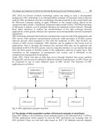
1.1 The configuration of wastewater treatment systems
The major sources of wastewater can be classified as municipal, industrial and agricultural.
Wastewater can be treated in wastewater treatment plants (WATP) or in decentralized
Waste Water - Evaluation and Management

182
wastewater treatment systems (DEWATS) (Jo & Mok, 2009). Wastewater can be described
using physical properties and by a list of chemical and biological constituents which should
be precisely specified (Muttamara, 1996). The physical properties of wastewater are
commonly listed as color, odor, turbidity, solids content and temperature. The wastewater
treatment and disposal commonly depends on water contamination with suspended solids,
biodegradable organics, pathogens, nutrients, refractory organics, dissolved inorganic solids
and heavy metals. The heavy metals are particularly present in industrial wastes. The
typical examples of refractory organics are surfactants, phenols and pesticides. While
phenols are present in industrial wastes, pesticides in agricultural wastes, surfactants are
common in households’ wastes. The surfactants (Abdel-Shafy et al., 1988) and oils tend to
resist conventional methods of wastewater treatment.
The properties of wastewater in the treatment process have to be monitored, particularly
before the effluent water is discharged to the environment. The commonly examined
parameters of wastewater before, during and after treatment in WATP are: pH, electric

conductivity (EC in µS), chemical oxygen demand (COD), biochemical oxygen demand
(BOD), total kjeldahl nitrogen (TKN mg/l), total organic carbon (TOC), total suspended
solids (TSS), and also bacteria presence (E. Coli- number/100ml) (Thomas et al., 1997). Users
of WATP run regular tests for those parameters.
DEWATS are intended for recycling domestic wastewater from individual households,
community plants and small industrial type systems producing effluent with similar
characteristics to domestic wastewater (Qadir et al., 2010). The objective of their operation is
efficient removal or conversion of the various types of pollutants that are present in
wastewater (Shirish et al., 2009). A typical DEWATS configuration is presented in Table 1.

Treatment Device Function
Settling tank
Septic tank
Primary
Anaerobic baffled reactor
Initial separation solids and liquid.
Solid matter or sewage disintegration
by bacteria.
Mechanical filter for example:
sand or membrane.
Secondary
Horizontal planted filter:
• filter media: pebbles with
top layer of sand,
• plant cover: Canna Indica
and Arundo Donax.
Filtration of wastewater to the
acceptable discharge standard.
UV electrically powered filter Reduction of bacteria and virus count.
Open collection tank

Finish
Open polishing tank
In the regions with high solarization the
collected water is naturally UV-filtered.
Table 1. Example of typical configuration of DEWATS
Domestic wastewater can be divided into grey and black wastewater. The grey wastewater
may be used directly for undersurface irrigation, when the irrigation does not cause
formation of ponds. It is recommended however that grey water should be treated before
use and that its contamination by surfactants should be tested. When the level of surfactants
in grey wastewater is high the discharge should be directed to sewage. The oil presented in
grey wastewater can block up the filters, so their condition also should be tested. The
Intelligent Photonic Sensors for Application in Decentralized Wastewater Systems

183
common way of treatment of grey and in some cases black wastewater is sedimentation
with microbiological disintegration in compact devices and mechanical filtration. Planted
vegetation is used sometimes for additional filtration. The UV light disintegration of
pathogens is also recommended as finishing treatment.
1.2 Sensors of parameters of liquids
There are many types of sensors that can be used for water and liquid monitoring, including
a wide range of fiber optic sensors with chemical or biological sensitive layers, and
electrochemical sensors that use fuel cells (Cusano et al., 2008). Under development are
sensor devices that could be used for wastewater monitoring: pH meters, conductivity
meters (EC), sensors for selected metal ion concentration, turbidity, liquid and sludge level
meters, flow meters, sensors of particle presence in flowing liquid and biosensors of aerobic
activated sludge organisms (Fazalul Rahiman & Abdul Rahim 2010) (Holtmann & Sell,
2002). The suspended solids concentrations and size distribution and particle weight can be
determined from turbidity measurements. The metal ion concentrations of dissolved oxygen
and carbon dioxide can be measured by using sensitive layers deposited on fiber tips or
inside of capillaries where they are optically monitored. The wastewater contamination with

toxic colony of micro organisms and BOD can be detected using fluorescence methods that
include adding a sensitive fluorescent liquid to the examined sample or by the
immobilization of a microbial layer on an amperometric oxygen electrode. The composition
of wastewater can be also monitored using near-infra-red (NIR) spectroscopy, but this
technique requires a laboratory setup and the set of reagents. Water contamination can be
also analyzed indirectly in the form of gas with the use of a chemical nose which is a matrix
sensor with integrated signal processing. There are sensors array systems intended for
monitoring volatile components of wastewater. In more advanced chemical noses the
wastewater sample is turned into vapor phase before the measurement is performed
(Bourgeois et al., 2003). In such systems the detector of the principal contaminating
component is used as the classifier of wastewater pollutants. The problem of
implementation of sensors in wastewater monitoring is mainly the cost of keeping the
sensor running or the time needed for examination and calibration.
1.3 The design objectives of DEWATS
Apart from technical aspects, the efficiency and the costs of the purification of wastewater,
which include the cost of wastewater examination, require serious consideration (Rulkens,
2008). The simple DEWATS configuration does not include sensors for discharge
monitoring, but as mentioned, the surfactants contamination and oil disintegration should
be tested. The operation of DEWATS should not require constant samples examination in a
laboratory. Therefore, DEWATS users need simple in use, low cost and fast sensing methods
for in-situ initial qualification of water treatment and discharge (Vanrolleghem & Lee, 2003).
Such methods would use sensors operating in a continuous mode without use of reagents,
and would feature simple or automatic head cleaning and regeneration. The sensors for
DEWATS have to be low cost in construction and operation and they have to enable
monitoring of surfactants presence and give a clear answer if the discharged water is
acceptable from environmental control point of view. Such requirements can be met by
physical methods of measurement using light or the electric current.
Waste Water - Evaluation and Management

184

2. Intelligent photonic sensors for wastewater treatment monitoring
In this work we present intelligent photonic sensors that can be used for monitoring of
wastewater treatment. These sensors work on the principle of optical intensity changes that
take place in dynamically forced measurement cycles. The sensors examine simultaneously
many liquid parameters which are processed in artificial neural networks (Borecki et al.,
2008a). The first type of sensors monitors signals from a drop forming during emerging and
after emergence of an optical fiber from the examined medium (Borecki, 2007). The second
type of sensors uses a fiber optical capillary in which the phase change from liquid to gas
and again to liquid is forced by local heating while the propagation of light across the
capillary where the liquid changes phase is monitored (Borecki et al., 2008b).
2.1 The examined liquids
To evaluate the proposed systems we used several liquids: still water, sparkling water, fresh
edible oil, spoiled edible oil and grey wastewater including in its composition commonly
present domestic discharge contaminants. We examined the still and sparkling waters
coming from this same source and producers. The sparkling water was saturated with
carbon dioxide. The detection of dissolved CO
2
is based on the measurements of differences
of the solubility of gases in water. Values of gas solubility in water are presented in Table 2.


Gas Solubility (ml/L)
Nitrogen 16.9
Oxygen 34.1
Methane CH
4
35
Carbon Dioxide CO
2
1019

Table 2. Examples of gas solubility in the water at 20°C
To simulate domestic grey wastewater with controllable composition we used water with
suspended solids (carbon powder), biodegradable organics (rapeseed oil, milk, fats),
nutrients (sugar, starch), and refractory organics (surfactants) and also dissolved inorganic
solids (some components of powder milk). We did not include in the composition heavy
metals and pathogens, but the pathogens can arise in the presence of milk, yogurt and
sugar, Table 3.


Type of contaminants Concentration of contaminant
Carbon powder 75 mg/l
Biodegradable surfactant 5ml/l
Rapeseed oil 10ml/l
Proteins with milk acid bacteria (Actimel) 1.25 ml/l
Proteins with fat (Powder milk 3.2% of fat) 1g/l
Starch (Flour) 1g/l
Sugar 1g/l
Table 3. Composition of the examined grey wastewater
The composition was treated for a few days in a still tank with a biological activator. We
used as activator a 1ml/l solution of 0.5 tablet which includes 4*108cfu of nonpathogenic
bacteria and enzymes that can disintegrate proteins, starch, oils, fats, papers and surfactants.
Intelligent Photonic Sensors for Application in Decentralized Wastewater Systems

185
After dissolving, the tablet works like a mixture of soda and vinegar. Our still tank was kept
at 26°C and had a volume of 5 liters and a height of 30cm. The sample for examination was
probed from the middle part of tank using a pipette. The changes in the liquid in 4 days of
probing in terms of pH and capillary action, which was measured in a glass capillary with a
diameter of 536μm, are presented in Table 4. The visualization of bacteria growth during the
treatment is presented in Fig. 1.



Treatment [day] pH Capillary action in [mm]
0 6.908 25.6
1 7.925 25.3
2 7.912 27.0
3 8.168 26.6

Table 4. pH and capillary action of grey wastewater in the function of treatment holding
time
The measured pH of the sample 1 day after preparation was about 8 and remained stable
during the following days, while initially the pH of the water was 7.0. The capillary action
remained stable at the average level of 26mm, while the capillary action of clear water was
about 39mm



0 days treatment 1 day treatment


2 days treatment 3 days treatment

Fig. 1. Visualization of bacteria growth as function of treatment holding time
The microscopic examination in the following days showed that our gray wastewater has
slightly increased number of bacteria. Therefore, we see that after 3 days of treatment our
gray wastewater which sediments in tank quite effectively, was not fresh drinkable water.
Waste Water - Evaluation and Management

186
2.2 Experimental setup

2.2.1 General description
We used two experimental setups, both with intelligent optoelectronic multi-parametric
signal detection (Borecki et al., 2008a). Both examined sensors used light intensity
measurements in forced measuring cycles and they used electrically controlled actuation to
generate time-dependant information (Borecki et al., 2010). In their construction we used to
the extent possible commercially available components.
The light source, and detection hardware were the same in both constructions. The heads
were optically connected using large core SMA optical connectors. As light source we used a
fiber coupled laser source S1FC635 from THORLABS that was coupled to the sensing head
with a multi-mode optical path-cord finished with FC connectors and FC to SMA mating
sleeves. The S1FC635 enabled light power stabilization and adjustments of power in the
range from 0.01mW to 2mW. We eliminated the effect of the ambient light by modulating
the probing light with 1kHz by connecting electrically a DG2021A function generator to the
modulation input of S1FC635. The scheme of the light source is presented in Fig. 2.


Fiber coupled laser source
S1FC635
Electrical socket BNC
Optical socket FC
Function generator
DG 2021A
Electrical socket BNC
FC/SMA
Pathcord FC
Fiber
to head
connection

Fig. 2. The light source used in experiments

In our experiments we used the optical signal from a S1FC635 LD at a level from 0.01 to
0.2mW. The signal was transmitted almost without losses to the head by a SMA socket. The
presented light power coupled into large core fibers could be also realized using properly
selected LED diodes powered from an electric driver which consisted of a laboratory power
supply that had precise output current settings and a transistor switch connected to the
generator.
The detection hardware consisted of an optoelectronic interface, a data acquisition system,
an electric actuation system and a PC with software, as shown on Fig. 3.

Optoelectronic
interface
Electrical output BNC
SMA Optical input socket
Data acquisition system
Personal Daq/3001
Data exange USB
Digital output Screw
Analog input S crew
PC with software:
- DASYLab 10 (data asquisition)
- Qnet (artificial neural network)
USB Data exange
Electric actuation system
Screw Digital input
Screw Electric power output
Optical fiber
from head
Electric connection
to actuation


Fig. 3. Scheme of the detection hardware
Intelligent Photonic Sensors for Application in Decentralized Wastewater Systems

187
The optoelectronic interface converted the intensity of amplitude modulated light into an
electric signal. First the light was converted to the electric signal by a photodiode that was
integrated in a trans-impedance circuit OP301. Then, all the components of the electric
spectrum that were not in the modulated band were filtered with the UAF42 circuit. Next,
the sensed changes of the modulated light intensity were demodulated with an AD536 true
RMS detector. The interface was sensitive for the changes of the modulated signal slower
that 5V/0.01s. The most expensive elements of the optoelectronic interface were the SMA
socket (about 16EUR distributor’s price) that was positioned mechanically directly above the
OP301 (50EUR).

The signal from the optoelectronic interface was fed to the data acquisition system that read
analog signals and converted them to the digital form proper for processing in the data
acquisition software. We used DASYLab software with two scripts. The first DASYLab
script was developed for data acquisition and the second was aimed for data classification.
The data were analyzed with 0.1second time base and were observed and converted to the
form required in the artificial neural network (ANN) Qnet microcontroller with embedded
software. We used ANN that was in the form of multilayer perceptron, because this
configuration showed its high usability in signal classification in sensors technique, (Borecki
& Korwin-Pawlowski, 2010).
2.2.2 Fiber optic setup for fiber drop analysis (FDA)
The first sensing setup consisted of a mini-lift holding an optical fiber optic with a bare tip
as a measuring head. This setup is presented in Fig. 4 and we used it for intelligent fiber
drop analysis.

Linear
guideway

Fiber holder
Step motor
and controler
Signal from
electric actuation system
Moving sample
shelf
2cm bare fiber tip
Sample in vessel
TOSLink
2*1 coupler
SMA
SMA
TOSLink fiber with
SMA / TOSLink
connectors
To optoelectronic
interface
From
light source
Polymer optical fiber
in coating (TOSLink)

Fig. 4. Scheme of mini-lift sensing setup used for fiber drop analysis
In this setup we used a linear guideway type MLA0373-5HK1SKK from Wobit with a length
of 50cm powered by a 10W step motor 57BYGH804. The guideway and optical fiber of the
head were mounted on the wall for stability. On the guideway we fixed a vessel with a
sample of a volume of 100ml. We controlled the movement of the liquid sample in the
directions up and down with a tolerance of 0.1mm by using a data acquisition system and
software. This construction provided a stable optical path that resulted in a more repeatable

signal than the configuration with a moving fiber and a fixed vessel. We configured the
Waste Water - Evaluation and Management

188
optical path using slightly modified TOSLink standard elements. We found that present
polymer optical fibers can have their coating stripped easily from the fiber without damage
being inflicted to the cladding or to the core. The sensing arm was one half of TOSLink
pathcord type T-T from Vitalco PRC cut in half with stripped coating tip on 2cm length. The
connections from light source and to the optoelectronic interface were made from HC302-
200 Clicktronic pathcord cut in a half with mounted SMA connectors on the cut tips.
We have also considered using pathcords from different producers and found them
working not as well with TOSLink coupler, but we found only one type of TOSLink coupler
available on the market. Inside the coupler there were four fibers with slightly smaller
diameter than ½ of the TOSLink fiber which we put together on our head arm and each two
fibers were connected with the input and output arms as is presented in Fig. 5. Therefore,
the coupler was in fact a divider and gave us the coefficient of light coupling from the
source to the detection lower than 25%. We also evaluated the SMA BFL48-600 pathcord
from Thorlab which had a core diameter 600μm, cladding diameter 630μm, coating diameter
1040μm and numerical aperture (NA): 0.48 ± 0.02 and a multimode FC pathcord with core
62.5mm for making the asymmetrical coupler presented in Fig. 5.

A) TOSLink B) Home-made asymmetrical
Connector
to head
Connector
to light
source
Connector
to optoel.
interface

Casing
4 fibers
BFL48-600 fiber
SMA connector
to optoel. interface
Direct path to head
φ
=0.6mm
FC connector
direct to
laser S1FC635
MM fiber62.5mm
1mm


Fig. 5. The two variants of couplers: A) – TOSLink, B) – Asymmetrical
The asymmetrical coupler had a coefficient of light coupling from the source to the detection
equal 43%, which was much higher than in the TOSLink construction, but the construction
with only TOSLink elements had still sufficient light power output and, moreover, the light
power balance in TOSLink did not decrease unacceptably when the LED light source was
tested. With the LED light source the asymmetrical coupler made from polymer fiber
presented in (Borecki, 2007) is recommended.
2.2.3 The setup for liquid-gas phase change measurements
The second sensing setup consisted of a head base, optical fibers, a miniature heater and a
disposable capillary. This setup is presented in Fig. 6 and we used it for intelligent liquid-
gas phase change capillary measurements.
Intelligent Photonic Sensors for Application in Decentralized Wastewater Systems

189
To electric

actuation system
To light source
V-grooves for
fibers
capillary
or
Capillary
base
Heater
Thermoelectric
temperature
controller
at the bottom
surface of plate
Aluminum
plate
Capillary optrode
with one end closed
Magnetic
tape
Optical
fiber

Optical
fiber
Cover
To opto-el. interface

Fig. 6. Scheme of capillary liquid-gas phase change sensing setup
In this setup we used capillaries TSP700850 from Polymicro Inc. and BFL48-600 optical

fibers with outer diameters of cladding similar. An important feature of the capillary probe
was that the top end of the capillary was blocked with the operator’s finger after the sample
was drawn and the bottom end contacted with liquid was blocked with modeling clay. This
prevented any sample spilling and ensured a safe transfer from the place of sample drawing
to the point of examination. The capillary had the length of 6cm and after introducing the
sampled liquid by capillary force to the length of about 20mm, modeling clay was inserted
to a length of a few millimeters to act as a stopper.
We used a SMA BFL48-600 fiber-tipped pathcord cut in a half. The stripped ends of the
fibers were mounted with mechanical clamps on the capillary base that was made from steel
with the tolerance of 2μm. The base was mounted on top of an aluminum plate. A
replaceable cover was put over the plate to prevent changes of heat transfer due to
uncontrolled air movement. On the bottom of the plate a thermoelectric temperature
controller was mounted to stabilize the temperature of the plate with an accuracy of 0.5°C.
The heater was made in thick film technology. The heating area was 1mm×3mm and the
heater could dissipate 10W in 60 second without degradation, with 6 minutes of
stabilization time required between temperature steps. The heater could generate a bubble
in the liquid filling the capillary above the middle or the edges of the heating area with the
bubble always moving towards the open end of capillary. Therefore, to avoid false
measurement results the observations were done above the edge of the heater closer to the
open tip of capillary.
2.3 Experimental results of fiber drop analysis (FDA)
The scheme with a mini-lift and a head with a bare POF fiber generated repeatable time-
domain signal waveforms. For example, during the examination of still water repeated 10
times it gave signals presented in Fig. 7. The signal can be analyzed considering two
Waste Water - Evaluation and Management

190
dynamic phases of the sensing head moving down (submerging) and up (emerging). When
the head during submerging crosses the liquid level the reflected signal decreases. The
signal drop depends on the indexes of refraction of the liquid and the fiber and on the

turbidity of the liquid. The signal decreases during first part of head emerging cycle. When
the head comes out of the liquid it takes with it a drop of the liquid. The signal behavior
next depends on the liquid’s parameters as: density, viscosity and surface tension related to
the fiber material which in this case should be not wetting. Probing of still water results in
formation of a drop that increases in volume and lasts for about 3 minutes when it comes
off. After that the signal returns to its initial level.


0.6
0.8
1
1.2
1.4
Time [s]
Signal [a.u.]
1
2
3
4
5
6
7
8
9
10
Still water sample No:
Submerging
Emerging
Emergence
Submersion

50 100 150 200 250 3000

Fig. 7. Signal collected in FDA for still water samples
In Fig. 8 is presented the signal collected from the solution of milk power in water at the
concentration of 500mg/l.

0 50 100 150 200 250 300
0.6
0.8
1
1.2
1.4
Time [s]
Signal [a.u.]
1
2
3
Still water TSS 500mg/l, sample No:

Fig. 8. Signals collected in FDA for samples of milk powder in still water at the
concentration of TSS = 500mg/l
Clearly, the signals presented in Fig. 7. and in Fig. 8. do not differ significantly. To simulate
closer the grey wastewater we added out-of-date edible refined rapeseed oil (without
chemical modifications) to the examined solution. We observed a 1mm thick coat of oil
forming on the water surface. The collected signals are presented in Fig. 9.
Intelligent Photonic Sensors for Application in Decentralized Wastewater Systems

191
0 50 100 150 200 250 300
0

0.5
1
1.5
2
2.5
3
3.5
4
Time [s]
Signal [a.u.]
1
2
3
4
5
6
7
9
Still water milk powder solution TSS 500mg/l
with 1mm oil coat on top surface, sample No:

Fig. 9. Signal collected in FDA for samples prepared of still water with milk powder in
concentration of TSS = 500mg/l and covered with 1mm out of date oil coat
The modification of the liquid sample with out of date oil introduces big differences
between the collected signals. The signals collected for liquid covered with 1mm thick coat
of fresh refined rapeseed oil are presented in Fig. 10.


0 50 100150200250300
0

1
2
3
4
5
6
Time [s]
Signal [a.u.]
1
2
3
4
5
6
7
8
9
Refined rapeseed oil, sample No:

Fig. 10. Signal collected in FDA for samples prepared of fresh refined rapeseed oil
The comparison of the characteristics from Fig. 9 and Fig. 10 leads us to the conclusion that
the signals from FDA for the samples of liquid with layer of fresh refined rapeseed oil are
repeatable, contrary to the signals collected from the layer of out-of-date oil on the surface of
water. We evaluated also the influence of a surfactant as water pollution agent. The
characteristics collected for a 5ml/l solution of biodegradable kitchen surfactant are
presented in Fig. 11.

Waste Water - Evaluation and Management

192

0 50 100 150 200 250 300
0
0.5
1
1.5
2
2.5
Time [s]
Signal [a.u]
Water with sufractant solution 5ml/l, sample No:
1
2
3
4
5
6
7
8
9

Fig. 11. Signal collected in FDA for water with biodegradable kitchen surfactant 5ml/l
solution
The last individual agent we examined that could be normally present in the wastewater
was carbon dioxide in the form of gas saturating bottled sparkling water. The following
samples were taken from the bottle in specified time in a period of about 6 minutes with the
time of opening the bottle was labeled 0min, as shown on Fig. 12.

0 50 100 150 200 250 300
0
0.5

1
1.5
2
2.5
3
Time [s]
Signal [a.u.]
0
6
12
19
25
33
40
46
51
58
Sparkling water, time from opening the bottle [min]:

Fig. 12. Signal collected in FDA for sparkling water
An observation can be made that in the presented method the water surfactant solution with
a concentration of 5ml/l and the sparkling water results in similar signals versus time
dependences. Similarly, washing objects is more efficient when using water with surfactant
or sparking water than still water.
Finally, we did tests with grey wastewater that was stored in a still tank for a few days. The
collected data are presented in Figs. 13-15.
Intelligent Photonic Sensors for Application in Decentralized Wastewater Systems

193


0 50 100 150 200 250 300
0
0.5
1
1.5
2
2.5
Time [s]
Signal [a.u.]
1
2
3 fiber head damage
4
5
6
7
8
9
10
11
Untreated grey wastewater, sample No:

Fig. 13. Signal collected in FDA for grey wastewater just after preparation
The data collected from raw grey wastewater just after preparation is presented in Fig. 13.
During that experiment we damaged the fiber head while cleaning it with a piece of tissue.
The damage was visible in the fiber cladding. The signal collected for next sample has lover
dynamics and increased level, which can be explained with changes in optical path
parameters due to fiber damage. The way to restore the head was simply to cut off the
damaged section, strip another fiber section and re-position the fiber tip. After this
procedure we collected the signals from the next samples. The signals collected for grey

wastewater that was treated in still tank for 1 day are presented in Fig. 14.


0 50 100 150 200 250 300
0
0.2
0.4
0.6
0.8
1
1.2
1.4
1.6
1.8
2
Time [s]
Signal [a.u]
Grey wastewater treated 1 day, sampe No
:
1
2
3
4
5
6
7
8
9
10


Fig. 14. Signal collected in FDA for grey wastewater that was treated in still tank for 1 day
The result of two days sample treatments is evident from comparison of data from Fig. 13 to
Fig. 15. Firstly, the examined wastewater just after preparation is not a homogeneous
mixture. This mixture stabilizes its parameters, but comparing Fig. 15, Fig. 7 and Fig. 11
gives us information that the presented treatment does not produce clear water which is in
accordance in biological examination shown on Fig. 1 and in Table 2. It is probable that the