[46] N. Wu, Y. Zhang, and K. Zhou. Detection, estimation, and accomodation of loss of
control effectiveness. Int. Journal of Adaptive Control and Signal Processing, 14:775–795,
2000.
[47] S. Wu, M. Grimble, and W. Wei. QFT based robust/fault tolerant flight control design
for a remote pilotless vehicle. In IEEE International Conference on Control Applications,
China, August 1999.
[48] S. Wu, M. Grimble, and W. Wei. QFT based robust/fault tolerant flight control
design for a remote pilotless vehicle. IEEE, Transactions on Control Systems Technology,
8(6):1010–1016, 2000.
[49] H. Yang, V. Cocquempot, and B. Jiang. Robust fault tolerant tracking control
with application to hybrid nonlinear systems. IET Control Theory and Applications,
3(2):211–224, 2009.
[50] X. Zhang, T. Parisini, and M. Polycarpou. Adaptive fault-tolerant control of nonlinear
uncertain systems: An information-based diagnostic approach. IEEE, Transactions on
Automatic Control, 49(8):1259–1274, 2004.
[51] Y. Zhang and J. Jiang. Design of integrated fault detection, diagnosis and reconfigurable
control systems. In IEEE, Conference on Decision and Control, pages 3587–3592, 1999.
[52] Y. Zhang and J. Jiang. Integrated design of reconfigurable fault-tolerant control systems.
Journal of Guidance, Control, and Dynamics, 24(1):133–136, 2000.
[53] Y. Zhang and J. Jiang. Bibliographical review on reconfigurable fault-tolerant control
systems. In Proceeding of the 5th IFAC symposium on fault detection, supervision and safety
for technical processes, pages 265–276, Washington DC, 2003.
[54] Y. Zhang and J. Jiang. Issues on integration of fault diagnosis and reconfigurable
control in active fault-tolerant control systems. In 6th IFAC Symposium on fault detection
supervision and safety of technical processes, pages 1513–1524, China, August 2006.
308
Robust Control, Theory and Applications
Anna Filasová and Dušan Krokavec
Technical University of Košice
Slovakia

1. Introduction
The complexity of control systems requires the fault tolerance schemes to provide control of
the faulty system. The fault tolerant systems are that one of the more fruitful applications with
potential significance for those domains in which control must proceed while the controlled
system is operative and testing opportunities are limited by given operational considerations.
The real problem is usually to fix the system with faults so that it can continue its mission
for some time with some limitations of functionality. These large problems are known as the
fault detection, identification and reconfiguration (FDIR) systems. The practical benefits of
the integrated approach to FDIR seem to be considerable, especially when knowledge of the
available fault isolations and the system reconfigurations is used to reduce the cost and to
increase the control reliability and utility. Reconfiguration can be viewed as the task to select
these elements whose reconfiguration is sufficient to do the acceptable behavior of the system.
If an FDIR system is designed properly, it will be able to deal with the specified faults and
maintain the system stability and acceptable level of performance in the presence of faults.
The essential aspect for the design offault-tolerant control requiresthe conception ofdiagnosis
procedures that can solve the fault detection and isolation problem. The fault detection is
understood as a problem of making a binary decision either that something has gone wrong
or that everything is in order. The procedure composes residual signal generation (signals that
contain information about the failures or defects) followed by their evaluation within decision
functions, and it is usually achieved designing a system which, by processing input/output
data, is able generating the residual signals, detect the presence of an incipient fault and isolate
it.
In principle, in order to achieve fault tolerance, some redundancy is necessary. So far direct
redundancy is realized by redundancy in multiple hardware channels, fault-tolerant control
involve functional redundancy. Functional (analytical) redundancy is usually achieved by
design of such subsystems, which functionality is derived from system model and can be
realized using algorithmic (software) redundancy. Thus, analytical redundancy most often
means the use of functional relations between system variables and residuals are derived
from implicit information in functional or analytical relationships, which exist between
measurements taken from the process, and a process model. In this sense a residual is

a fault indicator, based on a deviation between measurements and model-equation-based
computation and model based diagnosis use models to obtain residual signals that are as a
rule zero in the fault free case and non-zero otherwise.
Design Principles of Active Robust
Fault Tolerant Control Systems

14
A fault in the fault diagnosis systems can be detected and isolated when has to cause a
residual change and subsequent analyze of residuals have to provide information about faulty
component localization. From this point of view the fault decision information is capable
in a suitable format to specify possible control structure class to facilitate the appropriate
adaptation of the control feedback laws. Whereas diagnosis is the problem of identifying
elements whose abnormality is sufficient to explain an observed malfunction, reconfiguration
can be viewed as a problem of identifying elements whose in a new structure are sufficient to
restore acceptable behavior of the system.
1.1 Fault tolerant control
Main task to be tackled in achieving fault-tolerance is design a controller with suitable
reconfigurable structure to guarantee stability, satisfactory performance and plant operation
economy in nominal operational conditions, but also in some components malfunction.
Generally, fault-tolerant control is a strategy for reliable and highly efficient control law
design, and includes fault-tolerant system requirements analysis, analytical redundancy
design (fault isolation principles) and fault accommodation design (fault control requirements
and reconfigurable control strategy). The benefits result from this characterization give a
unified framework that should facilitate the development of an integrated theory of FDIR
and control (fault-tolerant control systems (FTCS)) to design systems having the ability to
accommodate component failures automatically.
FTCS can be classified into two types: passive and active. In passive FTCS, fix controllers are
used and designed in such way to be robust against a class of presumed faults. To ensure this a
closed-loop system remains insensitive to certain faults using constant controller parameters
and without use of on-line fault information. Because a passive FTCS has to maintain the

system stability under various component failures, from the performance viewpoint, the
designed controller has to be very conservative. From typical relationships between the
optimality and the robustness, it is very difficult for a passive FTCS to be optimal from the
performance point of view alone.
Active FTCS react to the system component failures actively by reconfiguring control actions
so that the stability and acceptable (possibly partially degraded, graceful) performance of
the entire system can be maintained. To achieve a successful control system reconfiguration,
this approach relies heavily on a real-time fault detection scheme for the most up-to-date
information about the status of the system and the operating conditions of its components.
To reschedule controller function a fixed structure is modified to account for uncontrollable
changes in the system and unanticipated faults. Even though, an active FTCS has the potential
to produce less conservative performance.
The critical issue facing any active FTCS is that there is only a limited amount of reaction
time available to perform fault detection and control system reconfiguration. Given the fact of
limited amount of time and information, it is highly desirable to design a FTCS that possesses
the guaranteed stability property as in a passive FTCS, but also with the performance
optimization attribute as in an active FTCS.
Selected useful publications, especially interesting books on this topic (Blanke et al.,2003),
(Chen and Patton,1999), (Chiang et al.,2001), (Ding,2008), (Ducard,2009), (Simani et al.,2003)
are presented in References.
310
Robust Control, Theory and Applications
1.2 Motivation
A number of problems that arise in state control can be reduced to a handful of
standard convex and quasi-convex problems that involve matrix inequalities. It is
known that the optimal solution can be computed by using interior point methods
(Nesterov and Nemirovsky,1994) which converge in polynomial time with respect to the
problem size and efficient interior point algorithms have recently been developed for and
further development of algorithms for these standard problems is an area of active research.
For this approach, the stability conditions may be expressed in terms of linear matrix

inequalities (LMI), which have a notable practical interest due to the existence of powerful
numerical solvers. Some progres review in this field can be found e.g. in (Boyd et al.,1994),
(Herrmann et al.,2007), (Skelton et al.,1998), and the references therein.
In contradiction to the standard pole placement methods application in active FTCS design
there don’t exist so much structures to solve this problem using LMI approach (e.g.
see (Chen et al.,1999), (Filasova and Krokavec,2009), (Liao et al.,2002), (Noura et al.,2009)). To
generalize properties of non-expansive systems formulated as H
∞
problems in the bounded
real lemma (BRL) form, the main motivation of this chapter is to present reformulated design
method for virtual sensor control design in FTCS structures, as well as the state estimator
based active control structures for single actuator faults in the continuous-time linear MIMO
systems. To start work with this formalism structure residual generators are designed at first
to demonstrate the application suitability of the unified algebraic approach in these design
tasks. LMI based design conditions are outlined generally to posse the sufficient conditions
for a solution. The used structure is motivated by the standard ones (Dong et al.,2009), and in
this presented form enables to design systems with the reconfigurable controller structures.
2. Problem description
Through this chapter the task is concerned with the computation of reconfigurable feedback
u
(t), which control the observable and controllable faulty linear dynamic system given by the
set of equations
˙q
(t)=Aq(t)+B
u
u(t)+B
f
f(t) (1)
y
(t)=Cq(t)+D

u
u(t)+D
f
f(t) (2)
where q
(t) ∈ IR
n
, u(t) ∈ IR
r
, y(t) ∈ IR
m
,andf(t) ∈ IR
l
are vectors of the state, input,
output and fault variables, respectively, matrices A
∈ IR
n×n
, B
u
∈ IR
n×r
, C ∈ IR
m×n
,
D
u
∈ IR
m×r
, B
f

∈ IR
n×l
, D
f
∈ IR
m×l
are real matrices. Problem of the interest is to design
the asymptotically stable closed-loop systems with the linear memoryless state feedback
controllers of the form
u
(t)=−K
o
y
e
(t) (3)
u
(t)=−Kq
e
(t) −Lf
e
(t) (4)
respectively. Here K
o
∈ IR
r×m
is the output controller gain matrix, K ∈ IR
r×n
is the nominal
state controller gain matrix, L
∈ IR

r×l
is the compensate controller gain matrix, y
e
(t) is by
virtual sensor estimated output of the system, q
e
(t) ∈ IR
n
is the system state estimate vector,
and f
e
(t) ∈ IR
l
is the fault estimate vector. Active compensate method can be applied for such
systems, where

B
f
D
f

=

B
u
D
u

L (5)
311

Design Principles of Active Robust Fault Tolerant Control Systems
and the additive term B
f
f(t) is compensated by the term
−B
f
f
e
(t)=−B
u
Lf
e
(t) (6)
which implies (4). The estimators are then given by the set of the state equations
˙q
e
(t)=Aq
e
(t)+B
u
u(t)+B
f
f
e
(t)+J(y(t) −y
e
(t)) (7)
˙
f
e

(t)=Mf
e
(t)+N(y(t ) −y
e
(t)) (8)
y
e
(t)=Cq
e
(t)+D
u
u(t)+D
f
f
e
(t) (9)
where J
∈ IR
n×m
is the state estimator gain matrix, and M ∈ IR
l×l
, N ∈ IR
l×m
are the system
and input matrices of the fault estimator, respectively or by the set of equation
˙q
fe
(t)=Aq
fe
(t)+B

u
u
f
(t)+J(y
f
(t) − D
u
u
f
(t) − C
f
q
fe
(t)) (10)
y
e
(t)=E(y
f
(t)+(C − EC
f
)q
fe
(t) (11)
where E
∈ IR
m×m
is a switching matrix, generally used in such a way that E = 0,orE = I
m
.
3. Basic preliminaries

Definition 1 (Null space) Let E, E ∈ IR
h×h
,rank(E)=k < h be a rank deficient matrix. Then the
null space
N
E
of E is the orthogonal complement of the row space of E.
Proposition 1 (Orthogonal complement) Let E, E
∈ IR
h×h
,rank(E)=k < h be a rank deficient
matrix. Then an orthogonal complement E
⊥
of E is
E
⊥
= E
◦
U
T
2
(12)
where U
T
2
is the null space of E and E
◦
is an arbitrary matrix of appropriate dimension.
Proof. The singular value decomposition (SVD) of E, E
∈ IR

h×h
,rank(E)=k < h gives
U
T
EV =

U
T
1
U
T
2

E

V
1
V
2

=

Σ
1
0
12
0
21
0
22


(13)
where U
T
∈ IR
h×h
is the orthogonal matrix of the left singular vectors, V ∈ IR
h×h
is the
orthogonal matrix of the right singular vectors of E and Σ
1
∈ IR
k×k
is the diagonal positive
definite matrix of the form
Σ
1
= diag

σ
1
···σ
k

, σ
1
≥···≥σ
k
> 0 (14)
which diagonal elements are the singular values of E. Using orthogonal properties of U and

V,i.e.U
T
U = I
h
,aswellasV
T
V = I
h
,and

U
T
1
U
T
2


U
1
U
2

=

I
1
0
0I
2


, U
T
2
U
1
= 0 (15)
respectively, where I
h
∈ IR
h×h
is the identity matrix, then E can be written as
E
= UΣV
T
=

U
1
U
2


Σ
1
0
12
0
21
0

22


V
T
1
V
T
2

=

U
1
U
2


S
1
0
2

= U
1
S
1
(16)
312
Robust Control, Theory and Applications

where S
1
= Σ
1
V
T
1
. Thus, (15) and (16) implies
U
T
2
E = U
T
2

U
1
U
2


S
1
0
2

= 0 (17)
It is evident that for an arbitrary matrix E
◦
is

E
◦
U
T
2
E = E
⊥
E = 0 (18)
E
⊥
= E
◦
U
T
2
(19)
respectively, which implies (12). This concludes the proof.
Proposition 2. (Schur Complement) Let Q > 0, R > 0, S are real matrices of appropriate
dimensions, then the next inequalities are equivalent

QS
S
T
−R

< 0 ⇔

Q
+ SR
−1

S
T
0
0
−R

< 0 ⇔ Q + SR
−1
S
T
< 0, R > 0 (20)
Proof. Let the linear matrix inequality takes form

QS
S
T
−R

< 0 (21)
then using Gauss elimination principle it yields

ISR
−1
0I

QS
S
T
−R


I0
R
−1
S
T
I

=

Q
+ SR
−1
S
T
0
0
−R

(22)
Since
det

ISR
−1
0I

= 1 (23)
and it is evident that this transform doesn’t change negativity of (21), and so (22) implies (20).
This concludes the proof.
Note that in the next the matrix notations E, Q, R, S, U,andV be used in another context, too.

Proposition 3 (Bounded real lemma) For given γ
∈ IR and the linear system (1), (2) with f(t)=0
if there exists symmetric positive definite matrix P
> 0 such that
⎡
⎣
A
T
P + PA PB
u
C
T
∗−γ
2
I
r
D
T
u
∗∗−I
m
⎤
⎦
< 0 (24)
where I
r
∈ IR
r×r
, I
m

∈ IR
m×m
are the identity matrices, respectively then given system is
asymptotically stable.
Hereafter,
∗ denotes the symmetric item in a symmetric matrix.
Proof. Defining Lyapunov function as follows
v
(q(t)) = q
T
(t)Pq(t)+

t
0

y
T
(r)y(r) −γ
2
u
T
(r)u(r)

dr
> 0 (25)
where P
= P
T
> 0, P ∈ IR
n×n

, γ ∈ IR, and evaluating the derivative of v( q(t)) with respect to
t then it yields
˙
v
(q(t)) = ˙q
T
(t)Pq(t)+q
T
(t)P ˙q(t)+y
T
(t)y(t) −γ
2
u
T
(t)u(t) < 0
(26)
313
Design Principles of Active Robust Fault Tolerant Control Systems
Thus, substituting (1), (2) with f(t)=0 it can be written
˙
v
(q(t)) = (Aq(t)+B
u
u(t))
T
Pq(t)+q
T
(t)P(Aq(t)+B
u
u(t))+

+(
Cq(t)+D
u
u(t))
T
(Cq(t)+D
u
u(t)) −γ
2
u
T
(t)u(t) < 0
(27)
and with notation
q
T
c
(t)=

q
T
(t) u
T
(t)

(28)
it is obtained
˙
v
(q(t)) = q

T
c
(t)P
c
q
c
(t) < 0 (29)
where
P
c
=

A
T
P + PA PB
u
∗−γ
2
I
r

+

C
T
CC
T
D
u
∗ D

T
u
D
u

< 0 (30)
Since

C
T
CC
T
D
u
∗ D
T
u
D
u

=

C
T
D
T
u


CD

u

≥ 0 (31)
Schur complement property implies
⎡
⎣
00 C
T
∗ 0D
T
u
∗∗−I
m
⎤
⎦
≥ 0 (32)
then using (32) the LMI (30) can now be written compactly as (24). This concludes the proof.
Remark 1 (Lyapunov inequality) Considering Lyapunov function of the form
v
(q(t)) = q
T
(t)Pq(t) > 0 (33)
where P
= P
T
> 0, P ∈ IR
n×n
, and the control law
u
(t)=−K

o

y
(t) −D
u
u(t)

= −K
o
Cq(t) (34)
where K
o
∈ IR
r×m
is a gain matrix. Because in this case (27) gives
˙
v
(q(t)) = (Aq(t)+B
u
u(t))
T
Pq(t)+q
T
(t)P(Aq(t)+B
u
u(t)) < 0
(35)
then inserting (34) into (35) it can be obtained
˙
v

(q(t)) = q
T
(t)P
cb
q(t) < 0 (36)
where
P
cb
= A
T
P + PA −PB
u
K
o
C −(PB
u
K
o
C)
T
< 0 (37)
Especially, if all system state variables are measurable the control policy can be defined as
follows
u
(t)=−Kq(t) (38)
and (37) can be written as
A
T
P + PA − PB
u

K −(PB
u
K)
T
< 0 (39)
Note that in a real physical dynamic plant model usually D
u
= 0.
314
Robust Control, Theory and Applications
Proposition 4 Let for given real matrices F, G and Θ = Θ
T
> 0 of appropriate dimension a matrix
Λ has to satisfy the inequality
FΛ G
T
+ GΛ
T
F
T
−Θ < 0 (40)
then any solution of Λ can be generated using a solution of inequality

−FHF
T
−Θ FH + GΛ
T
∗−H

< 0 (41)

where H
= H
T
> 0 is a free design parameter.
Proof. If (40) yields then there exists a matrix H
−1
= H
−T
> 0suchthat
FΛ G
T
+ GΛ
T
F
T
−Θ + GΛ
T
H
−1
ΛG
T
< 0 (42)
Completing the square in (42) it can be obtained
(FH + GΛ
T
)H
−1
(FH + GΛ
T
)

T
−FHF
T
−Θ < 0 (43)
and using Schur complement (43) implies (41).
4. Fault isolation
4.1 Structured residual generators of sensor faults
4.1.1 Set of the state estimators
To design structured residual generators of sensor faults based on the state estimators, all
actuators are assumed to be fault-free and each estimator is driven by all system inputs and
all but one system outputs. In that sense it is possible according with given nominal fault-free
system model (1), (2) to define the set of structured estimators for k
= 1,2, ,m as follows
˙q
ke
(t)=A
ke
q
ke
(t)+B
uke
u(t)+J
sk
T
sk

y
(t) −D
u
u(t)


(44)
y
ke
(t)=Cq
ke
(t)+D
u
u(t) (45)
where A
ke
∈ IR
n×n
, B
uke
∈ IR
n×r
, J
sk
∈ IR
n×(m−1)
,andT
sk
∈ IR
(m−1)×m
takes the next form
T
sk
= I
mk

=
⎡
⎢
⎢
⎢
⎢
⎢
⎢
⎢
⎢
⎢
⎣
10
···00000··· 00
.
.
.
.
.
.
00
···01000··· 00
00
···00010··· 00
.
.
.
.
.
.

00
···00000··· 01
⎤
⎥
⎥
⎥
⎥
⎥
⎥
⎥
⎥
⎥
⎦
(46)
Note that T
sk
can be obtained by deleting the k-th row in identity matrix I
m
.
Since the state estimate error is defined as e
k
(t)=q(t) −q
ke
(t) then
˙e
k
(t)=Aq(t)+B
u
u(t) −A
ke

q
ke
(t) − B
uke
u(t) −J
sk
T
sk

y
(t) −D
u
u(t)

=
=(
A −A
ke
−J
sk
T
sk
C)q(t)+(B
u
−B
uke
)u(t)+A
ke
e
k

(t)
(47)
To obtain the state estimate error autonomous it can be set
A
ke
= A −J
sk
T
sk
C, B
uke
= B
u
(48)
315
Design Principles of Active Robust Fault Tolerant Control Systems
It is obvious that (48) implies
˙e
k
(t)=A
ke
e
k
(t)=(A −J
sk
T
sk
C)e
k
(t) (49)

(44) can be rewritten as
˙q
ke
(t)=(A −J
sk
T
sk
C)q
ke
(t)+B
u
u(t)+J
sk
T
sk

y
(t) −D
u
u(t)

=
=
Aq
ke
(t)+B
u
u(t)+J
sk
T

sk

y
(t) −(Cq
ke
(t)+D
u
u(t))

(50)
and (44), (45) can be rewritten equivalently as
˙q
ke
(t)=Aq
ke
(t)+B
u
u(t)+J
sk
T
sk

y
(t) −y
ke
(t)

(51)
y
ke

(t)=Cq
ke
(t)+D
u
u(t) (52)
Theorem 1 The k-th state-space estimator (52), (53) is stable if there exist a positive definite symmetric
matrix P
sk
> 0, P
sk
∈ IR
n×n
and a matrix Z
sk
∈ IR
n×(m−1)
such that
P
sk
= P
T
sk
> 0 (53)
A
T
P
sk
+ P
sk
A −Z

sk
T
sk
C −C
T
T
T
sk
Z
T
sk
< 0 (54)
Then J
sk
can be computed as
J
sk
= P
−1
sk
Z
sk
(55)
Proof. Since the estimate error is autonomous Lyapunov function of the form
v
(e
k
(t)) = e
T
k

(t)P
sk
e
k
(t) > 0 (56)
where P
sk
= P
T
sk
> 0, P
sk
∈ IR
n×n
can be considered. Thus,
˙
v
(e
k
(t)) = e
T
k
(t)(A −J
sk
T
sk
C)
T
P
sk

e
k
(t)+e
T
k
(t)P
sk
(A −J
sk
T
sk
C)e
k
(t) < 0
(57)
˙
v
(e
k
(t)) = e
T
k
(t)P
skc
e
k
(t) < 0 (58)
respectively, where
P
skc

= A
T
P
sk
+ P
sk
A −P
sk
J
sk
T
sk
C −(P
sk
J
sk
T
sk
C)
T
< 0 (59)
Using notation P
sk
J
sk
= Z
sk
(59) implies (54). This concludes the proof.
4.1.2 Set of the residual generators
Exploiting the model-based properties of state estimators the set of residual generators can be

considered as
r
sk
(t)=X
sk
q
ke
(t)+Y
sk
(y(t) −D
u
u(t)), k = 1, 2, . . . , m (60)
Subsequently
r
sk
(t)=X
sk

q
(t) −e
k
(t)

+ Y
sk
Cq(t)=(X
sk
+ Y
sk
C)q(t) −X

sk
e
k
(t) (61)
316
Robust Control, Theory and Applications
0 5 10 15 20 25
0
1
2
3
4
5
6
7
8
y(t)
t[s]


y
1
(t)
y
2
(t)
0 5 10 15 20 25
0
1
2

3
4
5
6
7
8
y(t)
t[s]


y
1
(t)
y
2
(t)
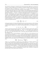
Fig. 1. Measurable outputs for single sensor faults
To eliminate influences of the state variable vector it is necessary in (61) to consider
X
sk
+ Y
sk
C = 0 (62)
Choosing X
sk
= −T
sk
C (62) implies
X
sk

= −T
sk
C, Y
sk
= T
sk
(63)
Thus, the set of residuals (60) takes the form
r
sk
(t)=T
sk

y
(t) −D
u
u(t) −Cq
ke
(t)

, k
= 1, 2, . . . , m (64)
When all actuators are fault-free and a fault occurs in the l -th sensor the residuals will satisfy
the isolation logic
r
sk
(t)≤h
sk
, k = l, r
sk

(t) > h
sk
, k = l (65)
This residual set can only isolate a single sensor fault at the same time. The principle can be
generalized based on a regrouping of faults in such way that each residual will be designed
to be sensitive to one group of sensor faults and insensitive to others.
Illustrative example
To demonstrate algorithm properties it was assumed that the system is given by (1), (2) where
the nominal system parameters are given as
A
=
⎡
⎣
010
001
−5 −9 −5
⎤
⎦
, B
u
=
⎡
⎣
13
21
15
⎤
⎦
, C
=


121
110

, D
u
=

00
00

and it is obvious that
T
s1
= I
21
=

01

, T
s2
= I
22
=

10

, T
s1

C =

110

, T
s2
C =

121

Solving (53), (54) with respect to the LMI matrix variables P
sk
,andZ
sk
using
Self-Dual-Minimization (SeDuMi) package for Matlab, the estimator gain matrix design
problem was feasible with the results
P
s1
=
⎡
⎣
0.8258
−0.0656 0.0032
−0.0656 0.8541 0.0563
0.0032 0.0563 0.2199
⎤
⎦
, Z
s1

=
⎡
⎣
0.6343
0.2242
−0.8595
⎤
⎦
, J
s1
=
⎡
⎣
0.8312
0.5950
−4.0738
⎤
⎦
317
Design Principles of Active Robust Fault Tolerant Control Systems
0 5 10 15 20 25
−20
−15
−10
−5
0
5
r
s1
(t)

t[s]


r
1
(t)
r
2
(t)
0 5 10 15 20 25
−40
−35
−30
−25
−20
−15
−10
−5
0
5
r
s2
(t)
t[s]


r
1
(t)
r

2
(t)
Fig. 2. Residuals for the 1st sensor fault
0 5 10 15 20 25
−20
−18
−16
−14
−12
−10
−8
−6
−4
−2
0
r
s1
(t)
t[s]


r
1
(t)
r
2
(t)
0 5 10 15 20 25
−40
−35

−30
−25
−20
−15
−10
−5
0
5
r
s2
(t)
t[s]


r
1
(t)
r
2
(t)
Fig. 3. Residuals for the 2nd sensor fault
P
s2
=
⎡
⎣
0.8258
−0.0656 0.0032
−0.0656 0.8541 0.0563
0.0032 0.0563 0.2199

⎤
⎦
, Z
s2
=
⎡
⎣
0.0335
0.6344
−0.9214
⎤
⎦
, J
s2
=
⎡
⎣
0.1412
1.0479
−4.4614
⎤
⎦
respectively. It is easily verified that the system matrices of state estimators are stable with the
eigenvalue spectra
ρ
(A −J
s1
T
s1
C)={−1.0000 −2.3459 −3.0804}

ρ(A −J
s2
T
s2
C)={−1.5130 −1.0000 −0.2626}
respectively, and the set of residuals takes the form
r
s1
(t)=

01


y
(t) −

121
110

q
ke
(t)

r
s2
(t)=

10



y
(t) −

121
110

q
ke
(t)

Fig. 1-3 plot the residuals variable trajectories over the duration of the system run. The results
show that one residual profile remain about the same through the entire run while the second
shows step changes, which can be used in the fault isolation stage.
318
Robust Control, Theory and Applications
4.2 Structured residual generators of actuator faults
4.2.1 Set of the state estimators
To design structured residual generators of actuator faults based on the state estimators, all
sensors are assumed to be fault-free and each estimator is driven by all system outputs and
all but one system inputs. To obtain this a congruence transform matrix T
ak
∈ IR
n×n
, k =
1, 2, . . . , r be introduced, and so it is natural to write
T
ak
˙q(t)=T
ak
Aq(t )+T

ak
B
u
u(t) (66)
˙q
k
(t)=A
k
q(t)+B
uk
u(t) (67)
respectively, where
A
k
= T
ak
A, B
uk
= T
ak
B
u
(68)
as well as
y
k
(t)=CT
ak
q(t)=Cq
k

(t) (69)
The set of state estimators associated with (67), (69) for k
= 1, 2, . . . ,r canbedefinedinthe
next form
˙q
ke
(t)=A
k
q
ke
(t)+B
uke
u(t)+L
k
y(t) −J
k
y
ke
(t) (70)
y
ke
(t)=Cq
ke
(t) (71)
A
ke
∈ IR
n×n
, B
uke

∈ IR
n×r
, J
k
, L
k
∈ IR
n×m
. Denoting the estimate error as e
k
(t)=q
k
(t) −q
ke
(t)
the next differential equations can be written
˙e
k
(t)= ˙q
k
(t) − ˙q
ke
(t)=
=
A
k
q(t)+B
uk
u(t) −A
k

q
ke
(t) −B
uke
u(t) −L
k
y(t)+J
k
y
ke
(t)=
=
A
k
q(t)+B
uk
u(t) −A
k

q
k
(t) − e
k
(t)

−B
uke
u(t)−
−
L

k
Cq(t)+J
k
C

q
k
(t) −e
k
(t)

=
=(
A
k
−A
k
T
ak
+ J
k
CT
ak
−L
k
C)q(t)+(B
uk
−B
uke
)u(t)+(A

k
−J
k
C)e
k
(t)
(72)
˙e
k
(t)=(T
ak
A −A
ke
T
ak
−L
k
C)q(t)+(B
uk
−B
uke
)u(t)+A
ke
e
k
(t) (73)
respectively, where
A
ke
= A

k
−J
k
C = T
ak
A −J
k
C, k = 1, 2, . . . , r (74)
are elements of the set of estimators system matrices. It is evident, to make estimate error
autonomous that it have to be satisfied
L
k
C = T
ak
A −A
ke
T
ak
, B
uke
= B
uk
= T
ak
B
u
(75)
Using (75) the equation (73) can be rewritten as
˙e
k

(t)=A
ke
e
k
(t)=(A
k
−J
k
C)e
k
(t)=(T
ak
A −J
k
C)e
k
(t) (76)
and the state equation of estimators are then
˙q
ke
(t)=(T
ak
A −J
k
C)q
ke
(t)+B
uk
u(t)+L
k

y(t) −J
k
y
ke
(t) (77)
y
ke
(t)=Cq
ke
(t) (78)
319
Design Principles of Active Robust Fault Tolerant Control Systems
4.2.2 Congruence transform matrices
Generally, the fault-free system equations (1), (2) can be rewritten as
˙q
(t)=Aq(t)+b
uk
u
k
(t)+
r
∑
h=1,h=k
b
uh
u
h
(t) (79)
˙y
(t)=C ˙q(t)+D

u
˙u(t)=CAq(t)+Cb
uk
u
k
(t)+D
u
˙u(t)+
r
∑
h=1,h=k
Cb
uh
u
h
(t) (80)
Cb
uk
u
k
(t)= ˙y(t ) −CAq(t) −D
u
˙u(t) −
r
∑
h=1,h=k
Cb
uh
u
h

(t) (81)
respectively. Thus, using matrix pseudoinverse it yields
u
k
(t) ˙=(Cb
uk
)
1

˙y
(t) − CAq(t) −D
u
˙u(t) −
r
∑
h=1,h=k
Cb
uh
u
h
(t)

(82)
and substituting (81)
b
uk
u
k
(t) ˙= b
uk

(Cb
uk
)
1
Cb
uk
u
k
(t) (83)

I
n
−b
uk
(Cb
uk
)
1
C

b
uk
u
k
(t) ˙= 0 (84)
respectively. It is evident that if
T
ak
= I
n

−b
uk
(Cb
uk
)
1
C , k = 1, 2, . . . , r (85)
influence of u
k
(t) in (77) be suppressed (the k-th column in B
uk
= T
ak
B
u
is the null column,
approximatively).
4.2.3 Estimator stability
Theorem 2 The k-th state-space estimator (77), (78) is stable if there exist a positive definite symmetric
matrix P
ak
> 0, P
ak
∈ IR
n×n
and a matrix Z
ak
∈ IR
n×m
such that

P
ak
= P
T
ak
> 0 (86)
A
T
T
ak
P
ak
+ P
ak
T
ak
A −Z
ak
C −C
T
Z
T
ak
< 0 (87)
Then J
k
can be computed as
J
k
= P

−1
ak
Z
ak
(88)
Proof. Since the estimate error is autonomous Lyapunov function of the form
v
(e
k
(t)) = e
T
k
(t)P
ak
e
k
(t) > 0 (89)
where P
ak
= P
T
ak
> 0, P
ak
∈ IR
n×n
can be considered. Thus,
˙
v
(e

k
(t)) = e
T
k
(t)(T
ak
A −J
k
C)
T
P
ak
e
k
(t)+e
T
k
(t)P
ak
(T
ak
A −J
k
C)e
k
(t) < 0
(90)
˙
v
(e

k
(t)) = e
T
k
(t)P
akc
e
k
(t) < 0 (91)
respectively, where
P
akc
= A
T
T
T
ak
P
ak
+ P
ak
T
ak
A −P
ak
J
k
C −(P
ak
J

k
C)
T
< 0 (92)
Using notation P
ak
J
k
= Z
ak
(92) implies (87). This concludes the proof.
320
Robust Control, Theory and Applications
4.2.4 Estimator gain matrices
Knowing J
k
, k = 1, 2, . . . , r elements of this set can be inserted into (75). Thus
L
k
C = A
k
−A
ke
T
ak
= A
k
−

A

k
−J
k
C

I −b
uk
(Cb
uk
)
1
C

=
=

J
k
+

A
k
−J
k
C

b
uk
(Cb
uk

)
1

C
=

J
k
+ A
ke
b
uk
(Cb
uk
)
1

C
(93)
and
L
k
= J
k
+ A
ke
b
uk
(Cb
uk

)
1
, k = 1,2, ,r (94)
4.2.5 Set of the residual generators
Exploiting the model-based properties of state estimators the set of residual generators can be
considered as
r
ak
(t)=X
ak
q
ke
(t)+Y
ak
(y(t) −D
u
u(t)), k = 1, 2, . . . , m (95)
Subsequently
r
ak
(t)=X
ak

T
ak
q(t) −e
k
(t)

+ Y

ak
Cq(t)=(X
ak
T
ak
+ Y
ak
C)q(t) −X
ak
e
k
(t) (96)
To eliminate influences of the state variable vector it is necessary to consider
X
ak
T
ak
+ Y
ak
C = 0 (97)
X
ak

I
n
−b
uk
(Cb
uk
)

1
C

+ Y
ak
C = 0 (98)
respectively. Choosing X
ak
= −C (98) gives
−

C
−Cb
uk
(Cb
uk
)
1
C

+ Y
ak
C = −(I
m
−Cb
uk
(Cb
uk
)
1

)C + Y
ak
C = 0 (99)
i.e.
Y
ak
= I
m
−Cb
uk
(Cb
uk
)
1
(100)
Thus, the set of residuals (95) takes the form
r
ak
(t)=(I
m
−Cb
uk
(Cb
uk
)
1
)y(t) −Cq
ke
(t) (101)
When all sensors are fault-free and a fault occurs in the l-th actuator the residuals will satisfy

the isolation logic
r
sk
(t)≤h
sk
, k = l, r
sk
(t) > h
sk
, k = l (102)
This residual set can only isolate a single actuator fault at the same time. The principle can be
generalized based on a regrouping of faults in such way that each residual will be designed
to be sensitive to one group of actuator faults and insensitive to others.
321
Design Principles of Active Robust Fault Tolerant Control Systems
0 5 10 15 20
−2
0
2
4
6
8
10
12
14
16
y(t)
t[s]



y
1
(t)
y
2
(t)
0 5 10 15 20
−4
−2
0
2
4
6
8
10
12
14
16
y(t)
t[s]


y
1
(t)
y
2
(t)
Fig. 4. System outputs for single actuator faults
0 5 10 15 20

−40
−35
−30
−25
−20
−15
−10
−5
0
5
r
a1
(t)
t[s]


r
1
(t)
r
2
(t)
0 5 10 15 20
−50
−40
−30
−20
−10
0
10

r
a2
(t)
t[s]


r
1
(t)
r
2
(t)
Fig. 5. Residuals for the 1st actuator fault
Illustrative example
Using the same system parameters as that given in the example in Subsection 4.1.2, the next
design parameters be computed
b
u1
=
⎡
⎣
1
2
1
⎤
⎦
,
(Cb
u1
)

1
=

0.1333 0.0667

, T
a1
=
⎡
⎣
0.8000
−0.3333 −0.1333
−0.4000 0.3333 −0.2667
−0.2000 −0.3333 0.8667
⎤
⎦
b
u2
=
⎡
⎣
3
1
5
⎤
⎦
,
(Cb
u2
)

1
=

0.0862 0.0345

, T
a2
=
⎡
⎣
0.6379
−0.6207 −0.2586
−0.1207 0.7931 −0.0862
−0.6034 −1.0345 0.5690
⎤
⎦
A
1
=
⎡
⎣
0.6667 2.0000 0.3333
1.3333 2.0000 1.6667
−4.3333 −8.0000 −4.6667
⎤
⎦
, A
2
=
⎡

⎣
1.2931 2.9655 0.6724
0.4310 0.6552 1.2241
−2.8448 −5.7241 −3.8793
⎤
⎦
Y
a1
=

0.2
−0.4
−0.4 0.8

, Y
a2
=

0.1379
−0.3448
−0.3448 0.8621

Solving (86), (87) with respect to the LMI matrix variables P
ak
,andZ
ak
using
322
Robust Control, Theory and Applications
0 5 10 15 20

−40
−35
−30
−25
−20
−15
−10
−5
0
5
r
a1
(t)
t[s]


r
1
(t)
r
2
(t)
0 5 10 15 20
−50
−40
−30
−20
−10
0
10

r
a2
(t)
t[s]


r
1
(t)
r
2
(t)
Fig. 6. Residuals for the 2nd actuator fault
Self-Dual-Minimization (SeDuMi) package for Matlab, the estimator gain matrix design
problem was feasible with the results
P
a1
=
⎡
⎣
0.7555
−0.0993 0.0619
−0.0993 0.7464 0.1223
0.0619 0.1223 0.3920
⎤
⎦
Z
a1
=
⎡

⎣
0.0257 0.7321
0.4346 0.2392
−0.7413 −0.7469
⎤
⎦
, J
1
=
⎡
⎣
0.3504 1.2802
0.9987 0.8810
−2.2579 −2.3825
⎤
⎦
, L
1
=
⎡
⎣
0.2247 1.2173
0.7807 0.7720
−2.8319 −2.6695
⎤
⎦
P
a2
=
⎡

⎣
0.6768
−0.0702 0.0853
−0.0702 0.7617 0.0685
0.0853 0.0685 0.4637
⎤
⎦
Z
a2
=
⎡
⎣
0.2127 0.9808
0.3382 0.0349
−0.6686 −0.4957
⎤
⎦
, J
2
=
⎡
⎣
0.5888 1.6625
0.6462 0.3270
−1.6457 −1.4233
⎤
⎦
, L
2
=

⎡
⎣
0.3878 1.5821
0.6720 0.3373
−2.6375 −1.8200
⎤
⎦
respectively. It is easily verified that the system matrices of state estimators are stable with the
eigenvalue spectra
ρ
(T
a1
A −J
1
C)={−1.0000 −1.6256 ±0.3775 i}
ρ(T
a2
A −J
2
C)={−1.0000 −1.5780 ±0.4521 i}
respectively, and the set of residuals takes the form
r
a1
(t)=

0.2
−0.4
−0.4 0.8

y

(t) −

121
110

q
1e
(t)
r
a2
(t)=

0.1379
−0.3448
−0.3448 0.8621

y
(t) −

121
110

q
2e
(t)
Fig. 4-6 plot the residuals variable trajectories over the duration of the system run. The results
show that both residual profile show changes through the entire run, therefore a fault isolation
has to be more sophisticated.
323
Design Principles of Active Robust Fault Tolerant Control Systems

5. Control with virtual sensors
5.1 Stability of the system
Considering a sensor fault then (1), (2) can be written as
˙q
f
(t)=Aq
f
(t)+B
u
u
f
(t) (103)
y
f
(t)=C
f
q
f
(t)+D
u
u
f
(t) (104)
where q
f
(t) ∈ IR
n
, u
f
(t) ∈ IR

r
are vectors of the state, and input variables of the faulty
system, respectively, C
f
∈ IR
m×n
is the output matrix of the system with a sensor fault, and
y
f
(t) ∈ IR
m
is a faulty measurement vector. This interpretation means that one row of C
f
is
null row.
Problem of the interest is to design a stable closed-loop system with the output controller
u
f
(t)=−K
o
y
e
(t) (105)
where
y
e
(t)=Ey
f
(t)+(C − EC
f

)q
fe
(t) (106)
K
o
∈ IR
r×m
is the controller gain matrix, and E ∈ IR
m×m
is a switching matrix, generally used
in such a way that E
= 0,orE = I
m
.IfE = 0 full state vector estimation is used for control,
if E
= I
m
the outputs of the fault-free sensors are combined with the estimated state variables
to substitute a missing output of the faulty sensor.
Generally, the controller input is generated by the virtual sensor realized in the structure
˙q
fe
(t)=Aq
fe
(t)+B
u
u
f
(t)+J(y
f

(t) − D
u
u
f
(t) − C
f
q
fe
(t)) (107)
The main idea is, instead of adapting the controller to the faulty system virtually adapt the
faulty system to the nominal controller.
Theorem 3 Control of the faulty system with virtual sensor defined by (103) – (107) is stable in the
sense of bounded real lemma if there exist positive definite symmetric matrices Q, R
∈ IR
n×n
,and
matrices K
o
∈ IR
r×m
, J ∈ IR
n×m
such that
⎡
⎢
⎢
⎢
⎣
Φ
1

QB
u
K
o
(C −EC
f
) −QB
u
K
o
E

C
f
−D
u
K
o
(C −EC
f
)

T
∗ Φ
2
0

D
u
K

o
(C −EC
f
)

T
∗∗ −γ
2
I
r
−

D
u
K
o
E

T
∗∗ ∗ −I
m
⎤
⎥
⎥
⎥
⎦
< 0 (108)
where
Φ
1

= Q

A −B
u
K
o
(C −EC
f
)

+

A
−B
u
K
o
(C −EC
f
)

T
Q (109)
Φ
2
= R

A −JC
f


+

A
−JC
f

T
R (110)
Proof. Assembling (103), (104), and (107) gives

˙q
f
(t)
˙q
fe
(t)

=

A0
JC
f
A −JC
f

q
f
(t)
q
fe

(t)

+

B
u
B
u

u
f
(t) (111)
y
f
(t)=C
f
q
f
(t)+D
u
u
f
(t) (112)
324
Robust Control, Theory and Applications
Thus, defining the estimation error vector
e
qf
(t)=q
f

(t) −q
fe
(t) (113)
as well as the congruence transform matrix
T
= T
−1
=

I0
I
−I

(114)
and then multiplying left-hand side of (111) by (114) results in
T

˙q
f
(t)
˙q
fe
(t)

= T

A0
JC
f
A −JC

f

T
−1
T

q
f
(t)
q
fe
(t)

+ T

B
u
B
u

u
f
(t) (115)

˙q
f
(t)
˙e
qf
(t)


=

A0
0A
−JC
f

q
f
(t)
e
qf
(t)

+

B
u
0

u
f
(t) (116)
respectively. Subsequently, inserting (105), (106) into (116), (112) gives

˙q
f
(t)
˙e

qf
(t)

=

A
−B
u
K
o
(C−EC
f
) B
u
K
o
(C−EC
f
)
0A−JC
f

q
f
(t)
e
qf
(t)

+


−B
u
K
o
E
0

y
e
(t) (117)
together with
y
f
(t)=

C
f
−D
u
K
o
(C−EC
f
) D
u
K
o
(C−EC
f

)


q
f
(t)
e
qf
(t)

−D
u
K
o
Ey
e
(t) (118)
and it is evident, that the separation principle yields.
Denoting
q
T
ε
(t)=

q
T
f
(t) e
T
qf

(t)

, w
ε
(t)=y
e
(t) (119)
A
ε
=

A
−B
u
K
o
(C −EC
f
) B
u
K
o
(C − EC
f
)
0A−JC
f

, B
ε

=

−B
u
K
o
E
0

(120)
C
ε
=

C
f
−D
u
K
o
(C −EC
f
) D
u
K
o
(C − EC
f
)


, D
ε
= −D
u
K
o
E (121)
To accept the separation principle a block diagonal symmetric matrix P
ε
> 0 is chosen, i.e.
P
ε
= diag

QR

(122)
where Q
= Q
T
> 0, R = R
T
> 0, Q, R ∈ IR
n×n
Thus, with (109), (110) it yields
P
ε
A
ε
+ A

T
ε
P
ε
=

Φ
1
QB
u
K
o
(C −EC
f
)
∗
Φ
2

, P
ε
B
ε
=

−QB
u
K
o
E

0

(123)
and inserting (121), (123), into (24) gives (108). This concludes the proof.
It is evident that there are the cross parameter interactions in the structure of (108). Since the
separation principle pre-determines the estimator structure (error vectors are independent on
the state as well as on the input variables), the controller, as well as estimator have to be
designed independent.
325
Design Principles of Active Robust Fault Tolerant Control Systems
5.2 Output feedback controller design
Theorem 4 (Unified algebraic approach) A system (103), (104) with control law (105) is stable if
there exist positive definite symmetric matrices P
> 0, Π = P
−1
> 0 such that

B
⊥
u
(AΠ + ΠA
T
)B
⊥T
u
B
⊥
u
ΠC
T

fi
∗−I
m

< 0, i = 0, 1,2, . , m (124)
⎡
⎢
⎣
C
•T⊥
fi

PA
+ A
T
P0
∗−γ
2
I
r

C
•T⊥T
fi
C
•T⊥
fi

C
T

fi
0

∗−I
m
⎤
⎥
⎦
< 0 i = 1, 2, . . . , m, E = I
m
(125)

C
T⊥
(PA + A
T
P)C
T⊥T
C
T⊥
C
T
fi
∗−I
m

< 0 i = 0, 1,2, . . . m, E = 0 (126)
where
C
•T⊥

fi
=

(C−EC
fi
)
T
E

⊥
(127)
and B
⊥
u
is the orthogonal complement to B
u
. Then the control law gain matrix K
o
exists if for obtained
P there exist a symmetric matrices H
> 0 such that

−FHF
T
−Θ
i
FH + G
i
K
T

o
∗−H

< 0 (128)
where i
= 0, 1,2, . . . , m, and
Θ
i
= −
⎡
⎣
PA
+ A
T
P0 C
T
fi
∗−γ
2
I
r
0
∗∗−I
m
⎤
⎦
< 0, F = −
⎡
⎣
PB

u
0
0
⎤
⎦
, G
=
⎡
⎣
(C−EC
fi
)
T
E
0
⎤
⎦
(129)
Proof. Considering e
q
(t)=0 then inserting Q = P (108) implies
⎡
⎢
⎣
Φ
1
−PB
u
K
o

E

C
f
−D
u
K
o
(C − EC
f
)

T
∗−γ
2
I
r
−

D
u
K
o
E

T
∗∗ −I
m
⎤
⎥

⎦
< 0 (130)
where
Φ
1
= P

A −B
u
K
o
(C −EC
f
)

+

A
−B
u
K
o
(C −EC
f
)

T
P (131)
For the simplicity it is considered in the next that D
u

= 0 (in real physical systems this
condition is satisfied) and subsequently (130), (131) can now be rewritten as
⎡
⎣
PA
+ A
T
P0 C
T
f
∗−γ
2
I
r
0
∗∗−I
m
⎤
⎦
−
−
⎡
⎣
PB
u
0
0
⎤
⎦
K

o

C
−EC
f
E0

−
⎡
⎣
(C−EC
f
)
T
E
0
⎤
⎦
K
T
o

B
T
u
P00

< 0
(132)
326

Robust Control, Theory and Applications
Defining the congruence transform matrix
T
v
= diag

P
−1
I
r
I
m

(133)
then pre-multiplying left-hand side and right-hand side of (132) by (133) gives
⎡
⎣
AP
−1
+ P
−1
A
T
0P
−1
C
T
f
∗−γ
2

I
r
0
∗∗−I
m
⎤
⎦
−
−
⎡
⎣
B
u
0
0
⎤
⎦
K
o

(C−EC
f
)P
−1
E0

−
⎡
⎣
P

−1
(C−EC
f
)
T
E
0
⎤
⎦
K
T
o

B
T
u
00

< 0
(134)
Since it yields
B
◦⊥
u
=
⎡
⎣
B
u
0

0
⎤
⎦
⊥
=
⎡
⎣
B
⊥
u
00
0I
r
0
00I
m
⎤
⎦
(135)
pre-multiplying left hand side of (134) by (135) as well as right-hand side of (134) by
transposition of (135) leads to inequalities
⎡
⎣
B
⊥
u
(AP
−1
+ P
−1

A
T
)B
⊥T
u
0B
⊥
u
P
−1
C
T
f
∗−γ
2
I
r
0
∗∗−I
m
⎤
⎦
< 0 (136)

B
⊥
u
(AP
−1
+ P

−1
A
T
)B
⊥T
u
B
⊥
u
P
−1
C
T
f
∗−I
m

< 0 (137)
respectively. Considering all possible structures C
fi
, i = 1,2, . . . , m associated with simple
sensor faults, as well as fault-free regime associated with the nominal matrix C
= C
f0
,then
using the substitution P
−1
= Π the inequality (136) implies (124).
Analogously, using orthogonal complement
C

◦T⊥
f
=
⎡
⎣
(C−EC
f
)
T
E
0
⎤
⎦
⊥
=
⎡
⎢
⎣

(C−EC
f
)
T
E

⊥
0
0I
m
⎤

⎥
⎦
=

C
•T⊥
f
0
∗ I
m

(138)
and pre-multiplying left-hand side of (132) by (138) and its right-hand side by transposition
of (138) results in
⎡
⎢
⎣
C
•T⊥
f

PA
+ A
T
P0
∗−γ
2
I
r


C
•T⊥T
f
C
•T⊥
f

C
T
f
0

∗−I
m
⎤
⎥
⎦
< 0 (139)
Considering all possible structures C
fi
, i = 1, 2, . . . , m (139) implies (125).
Inequality (125) takes a simpler form if E
= 0. Thus, now
C
◦T⊥
f
=
⎡
⎣
C

T
0
0
⎤
⎦
⊥
=
⎡
⎣
C
T⊥
00
0I
r
0
00I
m
⎤
⎦
(140)
327
Design Principles of Active Robust Fault Tolerant Control Systems
and pre-multiplying left-hand sides of (132) by (140) and its right-hand side by transposition
of (140) results in
⎡
⎣
C
T⊥
(PA + A
T

P)C
T⊥T
0C
T⊥
C
T
f
∗−γ
2
I
r
0
∗∗−I
m
⎤
⎦
< 0 (141)
which implies (126). This concludes the proof.
Solving LMI problem (124), (125), (126) with respect to LMI variable P,thenitispossibleto
construct (128), and subsequently to solve (127) defining the feedback control gain K
o
,andH
as LMI variables.
Note, (124), (125), (126) have to be solved iteratively to obtain any approximation P
−1
= Π.
This implies that these inequalities together define only the sufficient condition of a solution,
and so one from
(P, Π
−1

) can be used in design independently while verifying solution
using the latter. Since of an approximative solution the matrix Θ defined in (129) need not
be negative definite, and so it is necessary to introduce into (128) a negative definite matrix
Θ
◦
fi
as follows
Θ
◦
fi
= Θ
fi
−Δ < 0 (142)
where Δ
> 0.
If (124), (125), (126) is infeasible the principle can be modified based on inequalities regrouping
e.g. in such way that solving (124), (125), and (124), (126) separatively and obtaining two
virtual sensor structures (one for E
= 0 and other for E = I
m
). It is evident that virtual sensor
switching be more sophisticated in this case.
5.3 Virtual sensor design
Theorem 5 Virtual sensor (107) associated with the system (103), (104) is stable if there exist symmetric
positive definite matrix R
∈ IR
n×n
,andamatrixZ ∈ IR
n×m
,suchthat

R
= R
T
> 0 (143)
RA
+ A
T
R −ZC
fi
+ C
T
fi
Z
T
< 0, i = 0, 1,2, . , m (144)
The virtual sensor matrix parameter is then given as
J
= R
−1
Z (145)
Proof. Supposing that q
(t)=0 and D
u
= 0 then (108), (110) is reduced as follows
⎡
⎣
Φ
2
00
∗−γ

2
I
r
0
∗∗−I
m
⎤
⎦
< 0 (146)
R

A
−JC
f

+

A
−JC
f

T
R < 0 (147)
respectively. Thus, with the notation
Z
= RJ (148)
(147) implies (144). This concludes the proof.
328
Robust Control, Theory and Applications
Illustrative example

Using for E = 0 the same system parameters as that given in the example in Subsection 4.1.2,
then the next design parameters were computed
B
⊥
u
=

−0.8581 0.1907 0.4767

, C
T⊥
=

0.5774
−0.5774 0.5774

C
f0
=

121
110

, C
f1
=

000
110


, C
f2
=

121
000

Solving (124) and the set of polytopic inequalities (126) with respect to P, Π using the SeDuMi
package the problem was feasible and the matrices
P
=
⎡
⎣
0.6836 0.0569
−0.0569
0.0569 0.6836 0.0569
−0.0569 0.0569 0.6836
⎤
⎦
as well as H
= 0.1I
2
was used to construct the next ones
Θ
0
=
⎡
⎢
⎢
⎢

⎢
⎢
⎢
⎢
⎢
⎣
0.5688 0.9111
−3.0769 1 1
0.9111
−0.9100 −5.8103 2 1
−3.0769 −5.8103 −6.7225 1 0
−0.1
−0.1
1.0000 2.0000 1.0000
−1
1.0000 1.0000 0
−1
⎤
⎥
⎥
⎥
⎥
⎥
⎥
⎥
⎥
⎦
, Θ
1
, Θ

2
F
T
= −

0.7405 1.4810 0.7405 0 0 0 0
1.8234 1.1386 3.3044 0 0 0 0

, G
T
=

1210000
1100000

To obtain negativity of Θ
◦
fi
the matrix Δ = 4.94I
7
was introduced. Solving the set of polytopic
inequalities (128) with respect to K
o
the problem was also feasible and it gave the result
K
o
=

−0.0734 −0.0008
−0.1292 0.1307


which secure robustness of control stability with respect to all structures of output matrices
C
fi
, i = 0, 1,2. In this sense
ρ
(A −B
u
K
o
C)=

−1.0000 −1.3941 ±2.3919 i

ρ
(A − B
u
K
o
C
f1
)=

−1.0000 −2.2603 ±1.6601 i

ρ
(A − B
u
K
o

C
f2
)=

−1.0000 −1.1337 ±1.8591 i

Solving the set of polytopic inequalities (144) with respect to R, Z the feasible solution was
R
=
⎡
⎣
0.7188 0.0010 0.0016
0.0010 0.7212 0.0448
0.0016 0.0448 0.1299
⎤
⎦
, Z
=
⎡
⎣
−0.0006 0.4457
0.0117 0.0701
−0.0629 −0.5894
⎤
⎦
Thus, the virtual sensor gain matrix J was computed as
J
=
⎡
⎣

0.0002 0.6296
0.0473 0.3868
−0.5003 −4.6799
⎤
⎦
329
Design Principles of Active Robust Fault Tolerant Control Systems
0 5 10 15 20 25 30 35 40
−2
−1.5
−1
−0.5
0
0.5
1
y(t)
t[s]


y
1
(t)
y
2
(t))
0 5 10 15 20 25 30 35 40
−2.5
−2
−1.5
−1

−0.5
0
0.5
y
e
(t)
t[s]


y
e1
(t)
y
e2
(t))
Fig. 7. System output and its estimation
which secure robustness of virtual sensor stability with respect to all structures of output
matrices C
fi
, i = 0,1, 2. In this sense
ρ
(A − JC)=
⎡
⎣
−1.0000
−1.1656
−3.4455
⎤
⎦
, ρ

(A − JC
f1
)=
⎡
⎣
−1.0000
−1.2760
−3.7405
⎤
⎦
ρ
(A − B
u
K
o
C
f2
)=
⎡
⎣
−1.0000
−1.1337 + 1.8591 i
−1.1337 −1.8591 i
⎤
⎦
As was mentioned above the simulation results were obtained by solving the semi-definite
programming problem under Matlab with SeDuMi package 1.2, where the initial conditions
were set to
q
(0)=


0.2 0.2 0.2

T
, q
e
(0)=

000

T
respectively, and the control law in forced mode was
u
f
(t)=−K
o
y
e
(t)+w(t), w(t)=

−0.2 −0.2

T
Fig. 7 shows the trajectory of the system outputs and the trajectory of the estimate system
outputs using virtual sensor structure. It can be seen there a reaction time available to perform
fault detection and isolation in the trajectory of the estimate system outputs, as well as a
reaction time of control system reconfiguration in the system output trajectory. The results
confirm that the true signals and their estimation always reside between limits given by static
system error of the closed-loop structure.
6. Active control structures with a single actuator fault

6.1 Stability of the system
Theorem 6 Fault tolerant control system defined by (1) – (9) is stable in the sense of bounded real
lemma if there exist positive definite symmetric matrices Q, R
∈ IR
n×n
, S ∈ IR
l×l
,andmatrices
330
Robust Control, Theory and Applications
K ∈ IR
r×n
, L ∈ IR
r×l
, J ∈ IR
n×m
, M ∈ IR
l×l
, N ∈ IR
l×m
such that
⎡
⎢
⎢
⎢
⎢
⎢
⎢
⎣
Φ

11
QB
u
KQB
u
L00(C −D
u
K)
T
∗ Φ
22
R(B
f
−JD
f
) −(SNC)
T
00(D
u
K)
T
∗∗ Φ
33
−SM S (D
u
L)
T
∗∗ ∗ −γ
2
I

l
00
∗∗ ∗ ∗−γ
2
I
l
0
∗∗ ∗ ∗ ∗ −I
m
⎤
⎥
⎥
⎥
⎥
⎥
⎥
⎦
< 0 (149)
where
Φ
11
= Q(A −B
u
K)+(A − B
u
K)
T
Q, Φ
22
= R(A − JC)+(A −JC)

T
R (150)
Φ
33
= S(M −ND
f
)+(M − ND
f
)
T
S (151)
Proof. Considering equality
˙
f
(t)=
˙
f
(t) and assembling this equality with (1) – (4), and with
(7) – (9) gives the result
⎡
⎢
⎢
⎣
˙q
(t)
˙q
e
(t)
˙
f

(t)
˙
f
e
(t)
⎤
⎥
⎥
⎦
=
⎡
⎢
⎢
⎣
A
−B
u
KB
f
−B
u
L
JC A
−B
u
K −JC JD
f
B
f
−JD

f
−B
u
L
00 0 0
NC
−NC ND
f
M −ND
f
⎤
⎥
⎥
⎦
⎡
⎢
⎢
⎣
q
(t)
q
e
(t)
f(t)
f
e
(t)
⎤
⎥
⎥

⎦
+
⎡
⎢
⎢
⎣
0
0
˙
f
(t)
0
⎤
⎥
⎥
⎦
(152)
y
=

C
−D
u
KD
f
−D
u
L

⎡

⎢
⎢
⎣
q
(t)
q
e
(t)
f(t)
f
e
(t)
⎤
⎥
⎥
⎦
(153)
which can be written in a compact form as
˙q
α
(t)=A
α
q
α
(t)+f
α
(t) (154)
y
= C
α

q
α
(t) (155)
where
q
T
α
(t)=

q
T
(t) q
T
e
(t) f
T
(t) f
T
e
(t)

, f
T
α
(t)=

0
T
0
T

˙
f
T
(t) 0
T

(156)
A
α
=
⎡
⎢
⎢
⎣
A
−B
u
KB
f
−B
u
L
JC A
−B
u
K −JC JD
f
B
f
−JD

f
−B
u
L
00 0 0
NC
−NC ND
f
M −ND
f
⎤
⎥
⎥
⎦
(157)
C
α
=

C
−D
u
KD
f
−D
u
L

(158)
Using notations

e
q
(t)=q(t) −q
e
(t), e
f
(t)=f(t) −f
e
(t) (159)
where e
q
(t) is the error between the actual state and the estimated state, and e
f
(t) is the error
between the actual fault and the estimated fault, respectively then it is possible to define the
state transformation
q
β
(t)=Tq
α
(t)=
⎡
⎢
⎢
⎣
q
(t)
e
q
(t)

f(t)
e
f
(t)
⎤
⎥
⎥
⎦
, f
β
(t)=Tf
α
(t)=
⎡
⎢
⎢
⎣
0
0
˙
f
(t)
˙
f(t)
⎤
⎥
⎥
⎦
, T
= T

−1
=
⎡
⎢
⎢
⎣
I000
I
−I0 0
00I0
00I
−I
⎤
⎥
⎥
⎦
(160)
331
Design Principles of Active Robust Fault Tolerant Control Systems