Multi-Loop PID Control Design by Data-Driven Loop-Shaping Method 153
4. Data generation and design procedure
4.1 Data generation by filtering
Since the multi-loop PID controller contains many variables to be determined, many linear
constraints are necessary for the determination. Since one linear constraint (27) is derived
from one input-output response e
(t), y(t), t ∈ [0, T], many input output responses would be
necessary.
In order to obtain the plant response e
(t) and y(t), we may give the test input to w(t) of the
system (1)-(3) at the steady state, or to the reference r
(t) of the system described by
y
= Pe (40)
e
= K(r − y). (41)
Since the plant is m-input and m-output, m sets of responses e
(t) and y(t) may be necessary at
least. Therefore, we give a test input for the j th input
[w]
j
or [r]
j
and measure the input-output
response
{e(t), y(t)}, which are denoted by e
j
, y
j
. By iterating this experiment m times, m sets
of data e

j
, y
j
, j = 1,2, . . . , m are obtained.
Next, we will generate many fictitious data e
ij
(t), y
ij
(t), i = 1, 2, . . ., n
F
, j = 1,2, . . . , m by
e
ij
(t) = F
i
(s)e
j
(t) (42)
y
ij
(t) = F
i
(s)y
j
(t), t ∈ [0, T] (43)
where the filter F
i
(s) is a stable transfer function. Note that the notation F
i
(s)e

j
(t) means that
F
i
(s) filters each element of the m-dimensional vector e
j
(t).
From the assumptions that P is linear time-invariant and that the system is in the steady state
at t
= 0,
y
ij
(t) = P(s)e
ij
(t) (44)
is satisfied. Namely, the data e
ij
(t), y
ij
(t) can be considered as the input-output response of
the plant.
Remark 1 Even if the condition that P is linear time-invariant is not assumed, the above loop
shaping problem can be interpreted for a nonlinear plant as a problem with the weighted L
2
gain criterion given by
F
i
(s)e
2
< γ

1
F
i
(s)w
2
, i = 1, 2,. . . , n
F
. (45)
Namely, if a controller is falsified by the condition (17) for the filtered responses of a nonlinear
plant, we can say that the controller is falsified by the criterion (45).
Remark 2 From the previous discussions, the L
2
gain constraint (17) is evaluated for the fic-
titious disturbances w
(t) given by (20), i.e. w(t) = e(t) + Ky(t) for the data e(t) = e
ij
(t),
y
(t) = y
ij
(t), i = 1, 2, . . . , n
F
, j = 1, 2, . . . , m and the number of disturbances is N = n
F
m.
4.2 Filter selection
We use the next bandpass filters F
i
(s) for the sample frequencies ω
i

, i = 1, 2, ··· , n
F
.
F
i
(s) =
ˆ
ψ
(s/ω
i
) (46)
ˆ
ψ
(s) =

s
(s + α)
2
+ 1

4
(47)
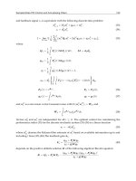
The gain plot of
ˆ
ψ(s) is shown in Fig. 3. Since the peak gain is taken at ω = ω
i
(1 + α
2
)
0.5

, this
filter can be used for extracting this frequency component.
Let us consider the filtering from the viewpoint of the wavelet transform (Addison (2002)).
In the last decade, wavelet transform has become popular as a time-frequency analysis tool.
Wavelet transform is useful to get important information regarding the frequency properties
lies locally in the time-domain from the non-stationary signals e, y .
If we denote the impulse response of F
i
(s) =
ˆ
ψ
(s/ω
i
) as L
−1
{F
i
(s)} = ω
i
ψ(ω
i
t) , then the
correspondence
a
↔
1
ω
i
, b ↔ t, −φ(−t) ↔ ψ(t). (48)
is satisfied between the filtering;

y
i
(t) = F
i
(s)y(t) (49)
= ω
i

t
0
ψ(ω
i
(t − τ))y(τ)dτ. (50)
and the integral wavelet transform;

W
φ
y

(b, a) = |a|
−1

∞
−∞
φ

τ
−b
a


y
(τ)dτ. (51)
The impulse response ψ
(t) of
ˆ
ψ(s) with α = 0.5 is shown in Fig. 4, and the graph of −φ
db10
(−t)
is shown in Fig. 5 for the Daubechies wavelet "db10"φ
db10
(t). From the uncertainty principle in
the wavelet analysis, there is a trade-off between the time window and the frequency window.
The time-frequency window can be tuned by the parameter α. α
= 0.5 is the value with which
ψ
(t) can be close to −φ
db10
(−t).
By the way, since F
i
(s) has four zeros at s = 0, F
i
(s)e(t) = 0 for e(t) = a
0
+ a
1
t + a
2
t
2

+ a
3
t
3
.
Namely, the output becomes zero for this class of smooth inputs. For step or ramp inputs,
their time-derivatives have discontinuity and so we have nonzero outputs. For the response
e
(t), y(t) shown in Fig. 6, the responses filtered by F
i
(s) are shown in Fig. 7.
4.3 Design procedure
Step 1 Measure the input output responses e
j
(t), y
j
(t), t ∈ [0, T], j = 1, 2, . . . , m by exciting
the system at the steady state. If the response has bias, eliminate it.
Step 2 Set ω
i
, i = 1, 2, . . . , n
F
as logarithmically equally spaced n
F
points in the important
frequency range for control. Generate the fictitious responses
e
ij
(t), y
ij

(t), t ∈ [0, T], i = 1, 2, . . . , n
F
. (52)
from e
j
(t), y
j
(t), t ∈ [0, T], j = 1, 2,. . . , m by (42) and (43). Set the value of γ
1
. Set the
value of γ
2
if necessary.
Step 3 Give a stabilizing PID gain
ˆ
K
a
that satisfies (17) and (18) for γ
1
and γ
2
. Then, com-
pute the constraints on the PID gains for the n
F
set of responses e
ij
(t), y
ij
(t) following
Theorems 1, 2, 3.

Step 4 If (17) is only considered as the constraints, solve a linear programming problem of
maximizing J subject to (13) and the linear constrains on the PID gains. Otherwise, if
both (17) and (18) are considered, solve an LMI problem of maximizing J defined by
(13) and the linear constrains on the PID gains.
PID Control, Implementation and Tuning154
10
−1
10
0
10
1
0
0.2
0.4
0.6
0.8
1
frequency w [rad/s]
gain |psihat(jw)|
Fig. 3. Gain plot of
ˆ
ψ(jω)
0 10 20 30 40 50
−0.2
−0.1
0
0.1
0.2
0.3
t

psi(t)
Fig. 4. Impulse response ψ(t) for σ = 0.5
0 5 10 15 20
−1
−0.5
0
0.5
1
1.5
tau
−psi(−tau)
Fig. 5. Mother wavelet db10 y = −φ
db10
(−τ)
0 20 40 60 80 100 120
−0.05
0
0.05
0.1
0.15
0.2
0.25
0.3
time
e and y
y(t)
e(t)
y(t)
e(t)
Fig. 6. e(t) and y(t)

0 20 40 60 80 100 120
−0.08
−0.06
−0.04
−0.02
0
0.02
0.04
0.06
0.08
time
Filtered y and e
ef(t)
yf(t)
Fig. 7. e
f
(t) = F
i
(s)e(t), y
f
(t) = F
i
(s)y(t)
Step 5 Implement the PID controller.
If the plant is stable, a low gain P or PD controller is usually a stabilizing PID gain
ˆ
K
a
that
satisfies (17) and (18) in Step 3. However, if the plant is marginally stable or unstable, it may

be not so easy to find such a stabilizing gain.
5. A numerical examples for a plant with time-delay
Let us consider the feedback system described by (40)(41), where the plant transfer function
is given by
P
(s) =

12.8
1
+16.7s
e
−s
18.9
1
+21s
e
−3s
6.6
1
+10.9s
e
−7s
19.4
1
+14.4s
e
−3s

. (53)
This transfer function is obtained from that of the Wood and Berry’s binary distillation column

process (Wood & Berry (1973)) by changing the sign of the
(1, 2 ) and (2, 2) elements so that
the plant may be stabilized by positive K
I
(1) and K
I
(2). Therefore, a solution for the Wood
and Berry’s binary distillation column process can be obtained by changing the sign of the
second PI controller designed by our method.
First, we will get the plant responses with a stabilizing controller K
(s) = 0.1I
2
. Measurement
noises with zero mean values and variances 0.0001 are given at the output y
1
and y
2
in the
closed-loop operation, respectively. Fig. 8 shows the response e
(t) and y(t) for the reference
input r
1
(t) = 1, r
2
(t) = 0, and Fig. 9 for r
1
(t) = 0, r
2
(t) = 1.
0 20 40 60 80 100

−0.2
0
0.2
0.4
0.6
time
y1, y2, e1,e2
Step response for r1=1
y1
y2
e1
e2
Fig. 8. Inputs and outputs of the plant for
r
1
(t) = 1 with K = 0.1I
2
0 20 40 60 80 100
−0.2
0
0.2
0.4
0.6
0.8
time
y1,y2,e1,e2
Step response for r2=1
e1
e2
y1

y2
Fig. 9. Inputs and outputs of the plant for
r
2
(t) = 1 with K = 0.1I
2
Now, design a diagonal PI controller using these step response data. We will only consider the
main constraint (17), and hence a solution can be obtained by applying linear programming.
We set γ
1
= 1.5 and ω
i
, i = 1,2, . . . ,40 logarithmically equally spaced frequencies between
0.1
[rad/s] and 10[rad/s], and give the bandpass filters by (46). The derivative and integral
calculations in the continuous time are executed approximately in the discrete time, where
the sampling interval is ∆T
= 0.05[s]. A solution that maximizes J = [K
I
]
11
+ [K
I
]
22
is given
by
K
(s) =


0.279
+
0.0368
s
0
0 0.0698
+
0.00834
s

. (54)
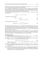
Fig. 10 shows the singular value plots of S
I
(s) and T
I
(s). In this figure, the horizontal line
shows the bound γ
1
= 1.5. Note that since the condition (17) is a necessary condition for
Multi-Loop PID Control Design by Data-Driven Loop-Shaping Method 155
10
−1
10
0
10
1
0
0.2
0.4
0.6

0.8
1
frequency w [rad/s]
gain |psihat(jw)|
Fig. 3. Gain plot of
ˆ
ψ(jω)
0 10 20 30 40 50
−0.2
−0.1
0
0.1
0.2
0.3
t
psi(t)
Fig. 4. Impulse response ψ(t) for σ = 0.5
0 5 10 15 20
−1
−0.5
0
0.5
1
1.5
tau
−psi(−tau)
Fig. 5. Mother wavelet db10 y = −φ
db10
(−τ)
0 20 40 60 80 100 120

−0.05
0
0.05
0.1
0.15
0.2
0.25
0.3
time
e and y
y(t)
e(t)
y(t)
e(t)
Fig. 6. e(t) and y(t)
0 20 40 60 80 100 120
−0.08
−0.06
−0.04
−0.02
0
0.02
0.04
0.06
0.08
time
Filtered y and e
ef(t)
yf(t)
Fig. 7. e

f
(t) = F
i
(s)e(t), y
f
(t) = F
i
(s)y(t)
Step 5 Implement the PID controller.
If the plant is stable, a low gain P or PD controller is usually a stabilizing PID gain
ˆ
K
a
that
satisfies (17) and (18) in Step 3. However, if the plant is marginally stable or unstable, it may
be not so easy to find such a stabilizing gain.
5. A numerical examples for a plant with time-delay
Let us consider the feedback system described by (40)(41), where the plant transfer function
is given by
P
(s) =

12.8
1+16.7s
e
−s
18.9
1+21s
e
−3s

6.6
1+10.9s
e
−7s
19.4
1+14.4s
e
−3s

. (53)
This transfer function is obtained from that of the Wood and Berry’s binary distillation column
process (Wood & Berry (1973)) by changing the sign of the
(1, 2 ) and (2, 2) elements so that
the plant may be stabilized by positive K
I
(1) and K
I
(2). Therefore, a solution for the Wood
and Berry’s binary distillation column process can be obtained by changing the sign of the
second PI controller designed by our method.
First, we will get the plant responses with a stabilizing controller K
(s) = 0.1I
2
. Measurement
noises with zero mean values and variances 0.0001 are given at the output y
1
and y
2
in the
closed-loop operation, respectively. Fig. 8 shows the response e

(t) and y(t) for the reference
input r
1
(t) = 1, r
2
(t) = 0, and Fig. 9 for r
1
(t) = 0, r
2
(t) = 1.
0 20 40 60 80 100
−0.2
0
0.2
0.4
0.6
time
y1, y2, e1,e2
Step response for r1=1
y1
y2
e1
e2
Fig. 8. Inputs and outputs of the plant for
r
1
(t) = 1 with K = 0.1I
2
0 20 40 60 80 100
−0.2

0
0.2
0.4
0.6
0.8
time
y1,y2,e1,e2
Step response for r2=1
e1
e2
y1
y2
Fig. 9. Inputs and outputs of the plant for
r
2
(t) = 1 with K = 0.1I
2
Now, design a diagonal PI controller using these step response data. We will only consider the
main constraint (17), and hence a solution can be obtained by applying linear programming.
We set γ
1
= 1.5 and ω
i
, i = 1,2, . . . ,40 logarithmically equally spaced frequencies between
0.1
[rad/s] and 10[rad/s], and give the bandpass filters by (46). The derivative and integral
calculations in the continuous time are executed approximately in the discrete time, where
the sampling interval is ∆T
= 0.05[s]. A solution that maximizes J = [K
I

]
11
+ [K
I
]
22
is given
by
K
(s) =

0.279
+
0.0368
s
0
0 0.0698
+
0.00834
s

. (54)
Fig. 10 shows the singular value plots of S
I
(s) and T
I
(s). In this figure, the horizontal line
shows the bound γ
1
= 1.5. Note that since the condition (17) is a necessary condition for

PID Control, Implementation and Tuning156
the L
2
gain constraint (9), the maximum singular value tends to become larger than γ
1
. Fig.
11 shows the step response y
(t) for the reference input r
1
(t) = 1, r
2
(t) = 0, and Fig. 12 for
r
1
(t) = 0, r
2
(t) = 1.
10
−3
10
−2
10
−1
10
0
10
1
10
−3
10

−2
10
−1
10
0
10
1
frequency[rad/s]
sigma(S), sigma(T)
Sigma plots
T
S
gam=1.5
Fig. 10. Singular value plots of S
I
and T
I
with PI control
0 20 40 60 80 100
−0.5
0
0.5
1
1.5
time
y1, y2
Step response for r1=1
y1
y2
Fig. 11. Output response of the plant for

r
1
(t) = 1 with PI control
0 20 40 60 80 100
−0.5
0
0.5
1
1.5
time
y1,y2
Step response for r2=1
y1
y2
Fig. 12. Output response of the plant for r
2
(t) =
1 with PI control
Next, design a diagonal PID controller with a first order lowpass filter of the next form using
the above plant responses. Note that our method can be directly applied to this design prob-
lem by considering the plant as P
(s)/(0.1s + 1). This filter is used for the attenuation of the
loop gain at high frequencies.
K
(s) =
1
0.1s + 1

K
P

+ K
I
1
s
+ K
D
s

(55)
Then, we obtain the next controller.
K
(s) =


0.383s+0.0798s+0.477s
2
(0.1s+1) s
0
0
0.118s+0.0246+0.247s
2
(0.1s+1) s


.
Fig. 13 shows the singular value plots, and Fig. 14 and Fig. 15 show the responses of the
closed-loop system for the reference inputs.
10
−2
10

−1
10
0
10
1
10
2
10
−3
10
−2
10
−1
10
0
10
1
frequency[rad/s]
sigma(S), sigma(T)
Sigma plots
S
T
gam=1.5
Fig. 13. Singular value plots of S
I
and T
I
with PID control
0 20 40 60 80 100
−0.5

0
0.5
1
1.5
time
y1, y2
Step response for r1=1
y1
y2
Fig. 14. Output response of the plant for
r
1
(t) = 1 with PID control
0 20 40 60 80 100
−0.5
0
0.5
1
1.5
time
y1,y2
Step response for r2=1
y1
y2
Fig. 15. Output response of the plant
for r
2
(t) = 1 with PID control
6. Experiment using a two-rotor hovering system
We will design a multi-loop PID controller for a two-rotor hovering system. The general view

of our experimental apparatus is shown in Fig.16. The arm AB can rotate around the center
O freely, and y
1
and y
2
are the yaw and the roll angles, respectively. The airframe CD can
also rotate freely on the axis AB, and θ is the pitch angle. Thus, this system has three degrees
of freedom. The rotors are driven separately by two DC motors. The rotary encoders are
mounted on the joint O to measure the angles y
1
and y
2
[rad], respectively. The encoder for θ
is mounted on the position A. The actuator part is illustrated in Fig. 17. The control inputs u
1
and u
2
are the thrust and the rolling moment, and
˜
f
1
and
˜
f
2
are the lift forces of the two rotors,
respectively. In our previous study , we designed a nonlinear controller for a mathematical
model (Saeki & Sakaue (2001)). Those who are interested in the plant property, please see the
reference.
The feedback control system is illustrated in Fig. 18. PID controller K will be designed to track

the references r
1
, r
2
[rad]. We use a PD controller 0.4 + 0.2s/ (1 + 0.01s) in order to control θ,
and this gain is determined by trail and error. Then, we treat the plant as a two-input two-
output system. The element denoted by K
uv
is a constant matrix that transforms the control
inputs u to the input voltages u
v
to the motors. The input voltages are limited to be less than
±5[V]. We consider the subsystem shown by the dotted line as the plant P to be controlled.
Multi-Loop PID Control Design by Data-Driven Loop-Shaping Method 157
the L
2
gain constraint (9), the maximum singular value tends to become larger than γ
1
. Fig.
11 shows the step response y
(t) for the reference input r
1
(t) = 1, r
2
(t) = 0, and Fig. 12 for
r
1
(t) = 0, r
2
(t) = 1.

10
−3
10
−2
10
−1
10
0
10
1
10
−3
10
−2
10
−1
10
0
10
1
frequency[rad/s]
sigma(S), sigma(T)
Sigma plots
T
S
gam=1.5
Fig. 10. Singular value plots of S
I
and T
I

with PI control
0 20 40 60 80 100
−0.5
0
0.5
1
1.5
time
y1, y2
Step response for r1=1
y1
y2
Fig. 11. Output response of the plant for
r
1
(t) = 1 with PI control
0 20 40 60 80 100
−0.5
0
0.5
1
1.5
time
y1,y2
Step response for r2=1
y1
y2
Fig. 12. Output response of the plant for r
2
(t) =

1 with PI control
Next, design a diagonal PID controller with a first order lowpass filter of the next form using
the above plant responses. Note that our method can be directly applied to this design prob-
lem by considering the plant as P
(s)/(0.1s + 1). This filter is used for the attenuation of the
loop gain at high frequencies.
K
(s) =
1
0.1s
+ 1

K
P
+ K
I
1
s
+ K
D
s

(55)
Then, we obtain the next controller.
K
(s) =


0.383s+0.0798s+0.477s
2

(0.1s+1) s
0
0
0.118s+0.0246+0.247s
2
(0.1s+1) s


.
Fig. 13 shows the singular value plots, and Fig. 14 and Fig. 15 show the responses of the
closed-loop system for the reference inputs.
10
−2
10
−1
10
0
10
1
10
2
10
−3
10
−2
10
−1
10
0
10

1
frequency[rad/s]
sigma(S), sigma(T)
Sigma plots
S
T
gam=1.5
Fig. 13. Singular value plots of S
I
and T
I
with PID control
0 20 40 60 80 100
−0.5
0
0.5
1
1.5
time
y1, y2
Step response for r1=1
y1
y2
Fig. 14. Output response of the plant for
r
1
(t) = 1 with PID control
0 20 40 60 80 100
−0.5
0

0.5
1
1.5
time
y1,y2
Step response for r2=1
y1
y2
Fig. 15. Output response of the plant
for r
2
(t) = 1 with PID control
6. Experiment using a two-rotor hovering system
We will design a multi-loop PID controller for a two-rotor hovering system. The general view
of our experimental apparatus is shown in Fig.16. The arm AB can rotate around the center
O freely, and y
1
and y
2
are the yaw and the roll angles, respectively. The airframe CD can
also rotate freely on the axis AB, and θ is the pitch angle. Thus, this system has three degrees
of freedom. The rotors are driven separately by two DC motors. The rotary encoders are
mounted on the joint O to measure the angles y
1
and y
2
[rad], respectively. The encoder for θ
is mounted on the position A. The actuator part is illustrated in Fig. 17. The control inputs u
1
and u

2
are the thrust and the rolling moment, and
˜
f
1
and
˜
f
2
are the lift forces of the two rotors,
respectively. In our previous study , we designed a nonlinear controller for a mathematical
model (Saeki & Sakaue (2001)). Those who are interested in the plant property, please see the
reference.
The feedback control system is illustrated in Fig. 18. PID controller K will be designed to track
the references r
1
, r
2
[rad]. We use a PD controller 0.4 + 0.2s/ (1 + 0.01s) in order to control θ,
and this gain is determined by trail and error. Then, we treat the plant as a two-input two-
output system. The element denoted by K
uv
is a constant matrix that transforms the control
inputs u to the input voltages u
v
to the motors. The input voltages are limited to be less than
±5[V]. We consider the subsystem shown by the dotted line as the plant P to be controlled.
PID Control, Implementation and Tuning158

encoder





y1
y
yy
y2
22
2
Fig. 16. Experimental setup
u

1
u

2
f
1
f
2



θ
θθ
θ
l
r
m


/

2
m

/

2


∼
∼∼
∼
∼
∼∼
∼
Fig. 17. Illustration of the actuator part
Thus, the feedback system is described by
y
= P(s)e (56)
e
= K(s)(r − y) (57)
The plant responses shown in Fig. 19 - Fig. 22 are obtained by experiment in the closed-loop
operation for the controller
K
(s) =

0.5 0
0 0.1


+

1 0
0 0

1
s
+

1 0
0 0.5

s
0.01s + 1
(58)
Now, let us design a PID controller by using the responses. Since this plant is marginally
stable, it is not so easy to give a stabilizing PID controller compared with stable plants. It is


+















+

θ





+


+







Fig. 18. Feedback control system
0 20 40 60
-0.2
0
0.2
0.4

e1
Step response(r1=0.2,r2=0)
0 20 40 60
−0.1
0
0.1
time[s]
e2
Fig. 19. Input response used for design
0 20 40 60
-0.1
0
0.1
0.2
0.3
time[s]
y1,y2[rad]
Step response(r1=0.2,r2=0)
y1
y2
Fig. 20. Output response used for design
0 20 40 60
-0.2
0
0.2
0.4
e1
Step response(r1=0,r2=0.5)
0 20 40 60
−0.2

0
0.2
time[s]
e2
Fig. 21. Input response used for design
0 20 40 60
-0.2
0
0.2
0.4
0.6
time[s]
y1,y2[rad]
Step response(r1=0,r2=0.5)
y1
y2
Fig. 22. Output response used for design
Multi-Loop PID Control Design by Data-Driven Loop-Shaping Method 159

encoder




y1
y
yy
y2
22
2

Fig. 16. Experimental setup
u

1
u

2
f
1
f
2



θ
θθ
θ
l
r
m

/

2
m

/

2



∼
∼∼
∼
∼
∼∼
∼
Fig. 17. Illustration of the actuator part
Thus, the feedback system is described by
y
= P(s)e (56)
e
= K(s)(r − y) (57)
The plant responses shown in Fig. 19 - Fig. 22 are obtained by experiment in the closed-loop
operation for the controller
K
(s) =

0.5 0
0 0.1

+

1 0
0 0

1
s
+


1 0
0 0.5

s
0.01s
+ 1
(58)
Now, let us design a PID controller by using the responses. Since this plant is marginally
stable, it is not so easy to give a stabilizing PID controller compared with stable plants. It is


+














+

θ






+


+







Fig. 18. Feedback control system
0 20 40 60
-0.2
0
0.2
0.4
e1
Step response(r1=0.2,r2=0)
0 20 40 60
−0.1
0
0.1
time[s]
e2
Fig. 19. Input response used for design

0 20 40 60
-0.1
0
0.1
0.2
0.3
time[s]
y1,y2[rad]
Step response(r1=0.2,r2=0)
y1
y2
Fig. 20. Output response used for design
0 20 40 60
-0.2
0
0.2
0.4
e1
Step response(r1=0,r2=0.5)
0 20 40 60
−0.2
0
0.2
time[s]
e2
Fig. 21. Input response used for design
0 20 40 60
-0.2
0
0.2

0.4
0.6
time[s]
y1,y2[rad]
Step response(r1=0,r2=0.5)
y1
y2
Fig. 22. Output response used for design
PID Control, Implementation and Tuning160
easier to find a stabilizing PD controller than PID controller. Therefore, we give the next PD
controller, which is found by trial and error.
K
a
=

0.4 0
0 0.4

+

1 0
0 0.5

s (59)
Sample frequencies ω
i
are logarithmically equally spaced 100 points between 10
−2
and 10
2

.
By solving an LMI once, we obtain the next controller.
K
(s) =

1.4549 0
0 1.0624

+

0.0980 0
0 0.1309

1
s
+

1.4914 0
0 1.2581

s
0.01s + 1
(60)
The step responses are shown in Fig. 23 - Fig. 26. It is necessary to develop an efficient method
of finding a stabilizing controller that satisfies (17)(18) for marginally stable or unstable plants.
This is our future work.
40 60 80 100
0
1
2

3
time[s]
e1,e2
e1
e2
Fig. 23. Input response(r1=0.2,r2=0)
40 60 80 100
-1
0
1
2
3
4
time[s]
e1,e2
e1
e2
Fig. 24. Input response(r1=0,r2=0.5)
40 60 80 100
-0.1
0
0.1
0.2
0.3
0.4
time[s]
y1,y2[rad]
y1
y2
Fig. 25. Output response 1 (r1=0.2,r2=0)

40 60 80 100
-0.2
0
0.2
0.4
0.6
0.8
time[s]
y1,y2[rad]
y2
y1
Fig. 26. Output response 2 (r1=0,r2=0.5)
7. Conclusion
DDLS (data driven loop shaping method) has been developed for the multi-loop PID control
tuning. The constraints on the PID gains are directly derived from a few input-output re-
sponses based on falsification conditions without explicitly identifying the plant model. The
design problem is reduced to a linear programming or a linear matrix inequality problem, and
the solution is obtained by solving it only once.
We have applied our method to the Wood and Berry’s binary distillation column process, and
our method gives good loop shapes where only two step responses of the closed-loop system
are used for design. However, it is difficult to specify the transient response property such as
overshoot by our method, because our method treats the optimization problem of disturbance
attenuation. Two-degree of freedom control systems may be suitable for the improvement of
the transient response. Further, we have applied our method to the control problem of a two-
rotor hovering system. From our experience including these examples, our method seems
considerably robust against noises of the plant input output signals obtained in the closed-
loop operation. Our design method can be extended to the PID controllers whose gains are
full square matrices.
8. References
Addison, P.S. (2002). The Illustrated Wavelet Transform Handbook, IOP Publishing Ltd., England.

Åström, K & Hägglund, T (1995). PID Controllers: Theory, Design, and Tuning, ISA, Research
Triangle Park, North Carolina.
Åström, K.; Panagopoulous, H.; Hägglund, T.(1998). Design of PI controllers based on non-
convex optimization, Automatica, pp. 585-601.
Åström, K & Hägglund, T (2006). Advanced PID Control, ISA.
Campi,M.C.; Lecchini, A.; Savaresi, S.M.(2002). Virtual reference feedback tuning: a direct
method for the design of feedback controllers, Automatica,Vol. 38, pp. 1337-1346.
Hjalmarsson, H.; Gevers, M.; Gunnarsson, S.;Lequin, O.(1999). Iterative feedback tuning: The-
ory and application, IEEE Control Systems Magazine, Vol. 42, No. 6, pp. 843-847.
Johnson, M.A. & Moradi, M.H. (Editors)(2005). PID Control; New identification and design meth-
ods, Springer-Verlag London Limited.
Lequin O.; Gevers M.; Mossberg M.; Bosmans E.; Triest L. (2003). Iterative feedback tuning of
PID parameters: comparison with classical tuning rules, Control Engineering Practice,
Vol. 11, pp. 1023-1033.
Saeki M. & Sakaue, Y. (2001). Flight control design for a nonlinear non-minimum phase VTOL
aircraft via two-step linearization, Proceedings of the 40th IEEE Conf. on Decision and
Control, pp. 217-222, Orland, Florida USA.
Saeki, M.(2004a). Unfalsified control approach to parameter space design of PID controllers,
Trans. of the Society of Instrument and Control Engineers, Vol. 40, No. 4, pp. 398-404.
Saeki,M.; Hamada, O.; Wada,N.; Masubuchi, I. (2006). PID gain tuning based on falsification
using bandpass filters, Proc. of SICE-ICCAS, Busan, Korea, pp. 4032–4037.
Saeki, M.(2008). Model-free PID controller optimization for loop shaping, Proc. of the 17th IFAC
World Congress, pp. 4958-4963.
Safonov, M.G. & Tsao, T.C. (1997). The unfalsified control concept and learning, IEEE Trans. on
Automatic Control, Vol. AC-42, No. 6, pp. 843-847.
Skogestad, S. & Postlethwaite, I. (2007), Multivariable Feedback Control, John Wiley & Sons, Ltd.
Multi-Loop PID Control Design by Data-Driven Loop-Shaping Method 161
easier to find a stabilizing PD controller than PID controller. Therefore, we give the next PD
controller, which is found by trial and error.
K

a
=

0.4 0
0 0.4

+

1 0
0 0.5

s (59)
Sample frequencies ω
i
are logarithmically equally spaced 100 points between 10
−2
and 10
2
.
By solving an LMI once, we obtain the next controller.
K
(s) =

1.4549 0
0 1.0624

+

0.0980 0
0 0.1309


1
s
+

1.4914 0
0 1.2581

s
0.01s
+ 1
(60)
The step responses are shown in Fig. 23 - Fig. 26. It is necessary to develop an efficient method
of finding a stabilizing controller that satisfies (17)(18) for marginally stable or unstable plants.
This is our future work.
40 60 80 100
0
1
2
3
time[s]
e1,e2
e1
e2
Fig. 23. Input response(r1=0.2,r2=0)
40 60 80 100
-1
0
1
2

3
4
time[s]
e1,e2
e1
e2
Fig. 24. Input response(r1=0,r2=0.5)
40 60 80 100
-0.1
0
0.1
0.2
0.3
0.4
time[s]
y1,y2[rad]
y1
y2
Fig. 25. Output response 1 (r1=0.2,r2=0)
40 60 80 100
-0.2
0
0.2
0.4
0.6
0.8
time[s]
y1,y2[rad]
y2
y1

Fig. 26. Output response 2 (r1=0,r2=0.5)
7. Conclusion
DDLS (data driven loop shaping method) has been developed for the multi-loop PID control
tuning. The constraints on the PID gains are directly derived from a few input-output re-
sponses based on falsification conditions without explicitly identifying the plant model. The
design problem is reduced to a linear programming or a linear matrix inequality problem, and
the solution is obtained by solving it only once.
We have applied our method to the Wood and Berry’s binary distillation column process, and
our method gives good loop shapes where only two step responses of the closed-loop system
are used for design. However, it is difficult to specify the transient response property such as
overshoot by our method, because our method treats the optimization problem of disturbance
attenuation. Two-degree of freedom control systems may be suitable for the improvement of
the transient response. Further, we have applied our method to the control problem of a two-
rotor hovering system. From our experience including these examples, our method seems
considerably robust against noises of the plant input output signals obtained in the closed-
loop operation. Our design method can be extended to the PID controllers whose gains are
full square matrices.
8. References
Addison, P.S. (2002). The Illustrated Wavelet Transform Handbook, IOP Publishing Ltd., England.
Åström, K & Hägglund, T (1995). PID Controllers: Theory, Design, and Tuning, ISA, Research
Triangle Park, North Carolina.
Åström, K.; Panagopoulous, H.; Hägglund, T.(1998). Design of PI controllers based on non-
convex optimization, Automatica, pp. 585-601.
Åström, K & Hägglund, T (2006). Advanced PID Control, ISA.
Campi,M.C.; Lecchini, A.; Savaresi, S.M.(2002). Virtual reference feedback tuning: a direct
method for the design of feedback controllers, Automatica,Vol. 38, pp. 1337-1346.
Hjalmarsson, H.; Gevers, M.; Gunnarsson, S.;Lequin, O.(1999). Iterative feedback tuning: The-
ory and application, IEEE Control Systems Magazine, Vol. 42, No. 6, pp. 843-847.
Johnson, M.A. & Moradi, M.H. (Editors)(2005). PID Control; New identification and design meth-
ods, Springer-Verlag London Limited.

Lequin O.; Gevers M.; Mossberg M.; Bosmans E.; Triest L. (2003). Iterative feedback tuning of
PID parameters: comparison with classical tuning rules, Control Engineering Practice,
Vol. 11, pp. 1023-1033.
Saeki M. & Sakaue, Y. (2001). Flight control design for a nonlinear non-minimum phase VTOL
aircraft via two-step linearization, Proceedings of the 40th IEEE Conf. on Decision and
Control, pp. 217-222, Orland, Florida USA.
Saeki, M.(2004a). Unfalsified control approach to parameter space design of PID controllers,
Trans. of the Society of Instrument and Control Engineers, Vol. 40, No. 4, pp. 398-404.
Saeki,M.; Hamada, O.; Wada,N.; Masubuchi, I. (2006). PID gain tuning based on falsification
using bandpass filters, Proc. of SICE-ICCAS, Busan, Korea, pp. 4032–4037.
Saeki, M.(2008). Model-free PID controller optimization for loop shaping, Proc. of the 17th IFAC
World Congress, pp. 4958-4963.
Safonov, M.G. & Tsao, T.C. (1997). The unfalsified control concept and learning, IEEE Trans. on
Automatic Control, Vol. AC-42, No. 6, pp. 843-847.
Skogestad, S. & Postlethwaite, I. (2007), Multivariable Feedback Control, John Wiley & Sons, Ltd.
PID Control, Implementation and Tuning162
Vidyasagar, M. (1993). Nonlinear systems analysis, second edition, PRENTICE HALL, Engle-
wood Cliffs.
Wood, R.K. & Berry, M.W. (1973). Terminal composition control of a binary distillation column,
Chem., Eng., Sci., Vo. 28, pp. 1707-1717, 1973.
Neural Network Based Tuning Algorithm for MPID Control 163
Neural Network Based Tuning Algorithm for MPID Control
Tamer Mansour, Atsushi Konno and Masaru Uchiyama
0
Neural Network Based Tuning
Algorithm for MPID Control
Tamer Mansour, Atsushi Konno and Masaru Uchiyama
Tohoku University
Japan
1. Introduction

One of the biggest problems for space manipulators are to cope with flexibility. If manipula-
tor links undergo deflection during the course of operation, it may prove difficult to reach a
desired position or to avoid obstacles. Furthermore, once the manipulator has reached a set
point, the residual vibration may degrade positioning accuracy and may cause a delay in task
execution. At the same time the flexible manipulators has the advantages of high payload to
weight ratio, which make them superior in the space exploration and orbital operation. The
high payl oad to weig ht ration is not the only merits of using flexible manipulators in space
application. Lower power consumption, smaller actuators and speedy operation make the
flexible manipulators the optimum choice for space manipulators. Since Cannon et al. (Can-
non & Schmitz, 1984) started initial experiments using the linear quadratic approach methods
to control flexible link manipulators, much researches on the usage of flexible manipulator
had been developed.
Using the approach of enhancement the measurements of the vibration variables was studied
by (Ge et al., 1999; Sun et al., 2005) while Etxebarria et al. (Etxebarria et al., 2005) gives attention
to the algorithms used in controlling the flexible manipulators. The enhancement of the tra-
ditional PD controller by adding a vibration control term is one of the most effective methods
for the flexible manipulators. L ee et al. proposed PDS (proportional-derivative strain) control
for vibration suppression of multi-flexible- link manipulators and analysed the Liapunov sta-
bility of the PDS control (Lee et al., 1988). Maruyama et al. (Maruyama et al., 2006) developed
a golf robot whose swing simulates human motion. They presented model accounting for golf
club flexibili ty with all parameters identified in experiments and generated and implemented
trajectories for different criterion such as minimizing total consumed work, minimizing sum-
mation o f the s quared derivative of active torque and maximizing impact speed. Matsuno and
Hayashi applied the PDS control to a cooperative task of two one-link flexible arms (Matsuno
& Hayashi, 2000). They aimed to accomplish the desired grasping force for a common rigid
object and the vibration absorption of the flexible arms.
A neural network is a data modelling tool that is able to capture and represent complex in-
put/output relationships. The motivation for the development of neural network technology
stemmed from the desire to develop an artificial system that could perform “intelligent" tasks
similar to those performed by the human brain. Neural Networks resemble the human brain

in the following two ways:
8
PID Control, Implementation and Tuning164
• A neural network acquires knowledge through learning.
• A neural network k nowledge is stored within inter neuron connection strengths known
as weights.
The true power and advantages of neural networks l ies in their ability to represe nt both linear
and non-linear relationships and in their ability to learn these relationships directly from the
data being modelled. Traditional linear models are simply inadequate when it comes to mod-
elling data that contains non-linear characteristics. Some researchers tried to use the neural
network (herein after abbreviated as NN) as a main controller like (Talebi et al., 1998). In their
research the controllers are designed by utilizing the modified output re-definition approach.
The modified output re-definition approach requires only a prior i knowledge about the lin-
ear model of the system but does not require a priori knowledge about the payload mass.
Various NN schemes have been proposed so far such as a modified version of the “feedback
error-learning" approach to lear n the inverse dynamics of the flexible manipulator (Kawato et
al., 1987). On the other proposed NN structure the controller is designed based on tracking
the reference joint angle while controlling the elastic deflection at the tip. Isogai et al. (Isogi
et al., 1999) proposed a fault-tolerant system using inverse dynamics constructed by NN for
sensor fault de tection and NN adaptive control for the actuator fault to reconfigure control to
compensate fo r parameter changes due to actuator faults.
Other researches like Lianfang (Lianfang et al., 2004) use the neural network as a correction
for the main control signal coming from the main feed-back controller. In his research the neu-
ral network approach is presented for the motion control of co nstrained flexible manipulators
where both the contact forces exerted by the flexible manipulator and the position of the end-
effectors contacting with a surface are controlled. Cheng and Patel in (Cheng & Patel, 2003)
tried to made stable tracking control of a flexible macro-micro manipulator utilizing two layer
neural network to approximate the non-linear robot dynamic behavior. A learning algorithm
for the neural network using Lyapunov stability is derived. Yazdizadeh et al. proposed two
neuro-dynamic identifiers to ide ntify the input-output relationship of two-link flexible manip-

ulator. They provided in (Yazdizadeh et al., 2000) a selection criterion for specifying the fixed
structural parameters as well as the adaptation laws fo r updating the adjustable parameters
of the networks .
A Modified PID control (MPID) is proposed to control a single-link flexible manipulator by
Mansour et al. (Mansour et al., 2008). The MPID control depends mainly on vibration feed-
back to improve the response of the flexible arm without the massive need of measurements.
The advantage of the MPID is that it is not affected by residual strain due to material defe ct
and/or static deformation. The residual strain and material defect may lead to inaccurate
movement. The difficulty with the MPID is that it includes nonlinear terms and so the stan-
dard gain tuning method can not be used for the controller. The motivation for this rese arch is
to find a fast and simple way to tune the MPID controller, which is able to achieve final accu-
rate tip position for the flexible arm and at the same time reduce resulting vibration. The NN
is use d to solve this problem. In this research a NN is used to find an optimum vibration gain
of MPID controller. The main advantage of the NN approach to tune the vibration control
gain of the MPID control is the considerable low computational cost to find an optimal tuned
gain with different tip payload.
The neural network is used to estimate a result of the dynamic simulation when the simulation
condition is given. As a result of the dynamic simulation, integral of the squared tip deflection
weighted by ex p onential function
Criterion function
=

t
s
0
δ
2
e
t
dt, t

s
: settling time (1)
is considered in this work. Therefore, the input to the neural network is the simulation con-
dition, while the output is the criterion f unction defined in 1. The mapping from the input
to the output is many-to-one. In order to train the neural network, the results of a dynamic
simulator for a given condition are us ed as teacher signals. In this shadow the feed-forward
neural network can be used as a mapping between the simulation conditions and the output
response all over the time span which is represented by

t
s
0
δ
2
e
t
dt.
The powerful ability of the neural network to model nonlinear model is utilized to map the
relation between the vibration control gain of the MPID and the output response represented
by the criterion function. Once this relation is drawn, the optimum value of the vibration
control gain is corresponding to the minimum value of the criterion function.
The sequence of finding the optimum value for the vibration control gain for the single link
flexible manipulator is summarized in Fig. 1. This chapter is organized as follows: An intro-
duction to the control of flexible manipulator and using NN in the control process is high-
lighted in section 1. The mathematical model of the flexible manipulator is shown in section
2. The detailed of the controller structure and the simulatiom model are prese nted in sections
3 and 4. In section 5 the NN algorithm used in this research is explained, the structure of the
NN is also shown and the optimal vibr ation control gain finding procedure are highlighted.
The learning and training process of the NN is shown in section 6. The response results for the
flexible manipulator with the tuned gain using the NN is shown in section 7. Finally, section

8 concludes this chapter with some remarks.
2. Mathematical Model
Before discussing the NN based gain tuning method, the MPID controller (Mansour et al.,
2008) is briefly introduced in sections 2 and 3. From the analysis of the single-link flexible arm
shown in Fig. 2, the flexible link is approximated by a continuous clamped- free beam. The
flexible arm is rotating in the horizontal plane with a rotational angle θ
(t) and the effect of
gravity is not take n into consideration. Frame O-XY is the fixed base frame and frame O-xy is
the local frame rotating with the hub. The tip deflection δ
(L, t) is the difference between the
actual tip position and the rotating frame O-xy. The deflection δ
(x, t) is assumed to be small
compared to the length of the arm. Let p
(x, t) represents the tangential position of a point
on the flexible arm with respect to frame O-xy. From the assumption of the deflection of the
flexible arm, the tangential position is expressed as:
p
(x, t) = xθ(t) + δ(x, t). (2)
The flexible arm is treated as Euler-Ber noull i beam with uniform cross-sectional area and con-
stant characteristics. Then, the Euler-Bernoulli equation for the link is given as follows :
EI
∂
4
p(x, t)
∂x
4
+ ρ
∂
2
p(x, t)

∂t
2
= 0, (3)
where ρ is the sectional d ensity, E is the Young (elastic) modulus, and I is the second mo ment
of area. Substituting (2) into (3) the following equation is obtained :
Neural Network Based Tuning Algorithm for MPID Control 165
• A neural network acquires knowledge through learning.
• A neural network k nowledge is stored within inter neuron connection strengths known
as weights.
The true power and advantages of neural networks l ies in their ability to represe nt both linear
and non-linear relationships and in their ability to learn these relationships directly from the
data being modelled. Traditional linear models are simply inadequate when it comes to mod-
elling data that contains non-linear characteristics. Some researchers tried to use the neural
network (herein after abbreviated as NN) as a main controller like (Talebi et al., 1998). In their
research the controllers are designed by utilizing the modified output re-definition approach.
The modified output re-definition approach requires only a prior i knowledge about the lin-
ear model of the system but does not require a priori knowledge about the payload mass.
Various NN schemes have been proposed so far such as a modified version of the “feedback
error-learning" approach to lear n the inverse dynamics of the flexible manipulator (Kawato et
al., 1987). On the other proposed NN structure the controller is designed based on tracking
the reference joint angle while controlling the elastic deflection at the tip. Isogai et al. (Isogi
et al., 1999) proposed a fault-tolerant system using inverse dynamics constructed by NN for
sensor fault de tection and NN adaptive control for the actuator fault to reconfigure control to
compensate fo r parameter changes due to actuator faults.
Other researches like Lianfang (Lianfang et al., 2004) use the neural network as a correction
for the main control signal coming from the main feed-back controller. In his research the neu-
ral network approach is presented for the motion control of co nstrained flexible manipulators
where both the contact forces exerted by the flexible manipulator and the position of the end-
effectors contacting with a surface are controlled. Cheng and Patel in (Cheng & Patel, 2003)
tried to made stable tracking control of a flexible macro-micro manipulator utilizing two layer

neural network to approximate the non-linear robot dynamic behavior. A learning algorithm
for the neural network using Lyapunov stability is derived. Yazdizadeh et al. proposed two
neuro-dynamic identifiers to ide ntify the input-output relationship of two-link flexible manip-
ulator. They provided in (Yazdizadeh et al., 2000) a selection criterion for specifying the fixed
structural parameters as well as the adaptation laws fo r updating the adjustable parameters
of the networks .
A Modified PID control (MPID) is proposed to control a single-link flexible manipulator by
Mansour et al. (Mansour et al., 2008). The MPID control depends mainly on vibration feed-
back to improve the response of the flexible arm without the massive need of measurements.
The advantage of the MPID is that it is not affected by residual strain due to material defe ct
and/or static deformation. The residual strain and material defect may lead to inaccurate
movement. The difficulty with the MPID is that it includes nonlinear terms and so the stan-
dard gain tuning method can not be used for the controller. The motivation for this rese arch is
to find a fast and simple way to tune the MPID controller, which is able to achieve final accu-
rate tip position for the flexible arm and at the same time reduce resulting vibration. The NN
is use d to solve this problem. In this research a NN is used to find an optimum vibration gain
of MPID controller. The main advantage of the NN approach to tune the vibration control
gain of the MPID control is the considerable low computational cost to find an optimal tuned
gain with different tip payload.
The neural network is used to estimate a result of the dynamic simulation when the simulation
condition is given. As a result of the dynamic simulation, integral of the squared tip deflection
weighted by ex p onential function
Criterion function
=

t
s
0
δ
2

e
t
dt, t
s
: settling time (1)
is considered in this work. Therefore, the input to the neural network is the simulation con-
dition, while the output is the criterion f unction defined in 1. The mapping from the input
to the output is many-to-one. In order to train the neural network, the results of a dynamic
simulator for a given condition are us ed as teacher signals. In this shadow the feed-forward
neural network can be used as a mapping between the simulation conditions and the output
response all over the time span which is represented by

t
s
0
δ
2
e
t
dt.
The powerful ability of the neural network to model nonlinear model is utilized to map the
relation between the vibration control gain of the MPID and the output response represented
by the criterion function. Once this relation is drawn, the optimum value of the vibration
control gain is corresponding to the minimum value of the criterion function.
The sequence of finding the optimum value for the vibration control gain for the single link
flexible manipulator is summarized in Fig. 1. This chapter is organized as follows: An intro-
duction to the control of flexible manipulator and using NN in the control process is high-
lighted in section 1. The mathematical model of the flexible manipulator is shown in section
2. The detailed of the controller structure and the simulatiom model are prese nted in sections
3 and 4. In section 5 the NN algorithm used in this research is explained, the structure of the

NN is also shown and the optimal vibration control gain finding procedure are highlighted.
The learning and training process of the NN is shown in section 6. The response results for the
flexible manipulator with the tuned gain using the NN is shown in section 7. Finally, section
8 concludes this chapter with some remarks.
2. Mathematical Model
Before discussing the NN based gain tuning method, the MPID controller (Mansour et al.,
2008) is briefly introduced in sections 2 and 3. From the analysis of the single-link flexible arm
shown in Fig. 2, the flexible link is approximated by a continuous clamped- free beam. The
flexible arm is rotating in the horizontal plane with a rotational angle θ
(t) and the effect of
gravity is not take n into consideration. Frame O-XY is the fixed base frame and frame O-xy is
the local frame rotating with the hub. The tip deflection δ
(L, t) is the difference between the
actual tip position and the rotating frame O-xy. The deflection δ
(x, t) is assumed to be small
compared to the length of the arm. Let p
(x, t) represents the tangential position of a point
on the flexible arm with respect to frame O-xy. From the assumption of the deflection of the
flexible arm, the tangential position is expressed as:
p
(x, t) = xθ(t) + δ(x, t). (2)
The flexible arm is treated as Euler-Ber noull i beam with uniform cross-sectional area and con-
stant characteristics. Then, the Euler-Bernoulli equation for the link is g iven as follows :
EI
∂
4
p(x, t)
∂x
4
+ ρ

∂
2
p(x, t)
∂t
2
= 0, (3)
where ρ is the sectional d ensity, E is the Young (elastic) modulus, and I is the second mo ment
of area. Substituting (2) into (3) the following equation is obtained :
PID Control, Implementation and Tuning166
Collect experimental or simulation results
Specify the output and input of the neural network
Select criteria function to represent output response
Train the neural network to get minimum value of the criteria function
Input the actual working data and get the optimal value for the output parameter
Specify the network structure (number of layers, training algorithm, )
Collect experimental or simulation results
Specify the output and input of the neural network
Train the neural network to get minimum value of the criteria function
Input the actual working data and get the optimal value for the output parameter
Specify the network structure (number of layers, training algorithm,
Fig. 1. Neural ne twork using sequence.
EI
∂
4
δ(x, t)
∂x
4
+ ρ
∂
2

δ(x, t)
∂t
2
= −ρx
¨
θ(t). (4)
The flexible arm is clamped at its base, so both the deflection and slope of the deflection curve
must be zero at the clamped end. Bending moment at the free end also equals zero. Making
force balance at the tip obtains the following boundary conditions:
δ
(x, t)
|
x=0
= 0, (5)
∂δ
(x, t)
∂x




x=0
= 0, (6)
EI
∂
2
δ(x, t)
∂x
2





x=L
= 0, (7)
EI
∂
3
δ(x, t)
∂x
3




x=L
= m
t

x
¨
θ
(t) +
∂
2
δ(x, t)
∂t
2

x=L

, (8)
where L is the arm l ength. The dynamic e quation describing the system presented in (?) is
written as foll ows:
T
(t) =

I
h
+
1
3
ρL
3

¨
θ
(t) + ρ

L
0
x
¨
δ(x, t)dx
+m
t
L

L
¨
θ(t) +

¨
δ
(L, t)

. (9)

y
X

Y
x
θ

p(x,t)
δ (x,t)
I
h
,
M
t

O
T
Fig. 2. Single-link flexible manipulator.
A flexible manipulator simulator is built in MATLAB Simulink software using the mathemat-
ical mod el shown before to study the performance of the MPID control with different loading
and gains conditions.
3. Controller
A Modified PID controller (MPID) is proposed for controlling the tip position of the single-
link flexible manipulator (Mansour et al., 2008). This controller used three measurements to

generate the control signal, the hub rotational angle θ
(t), the tip deflection δ(L, t) , and the
velocity of the hub
˙
θ
(t). If we choose the tip position as the output from the system then the
error includes two components. The first component e
j
(t) is a result of the joint motion and is
equal to L
(θ
re f
− θ(t)) which is identical with the rig id arm error where θ
re f
is the reference
joint angle. The second one is much more important and is due to the flexibility of the arm
and equals δ
(L, t). These two error components are coupled to each other. The Modified
PID (MPID) controller replaces the classical integral term of a PID controller with a vibration
feedback term to affect the flexible modes of the beam in the generated control signal. The
MPID controller is formed as follows (Mansour et al., 2008):
u
(t) = K
p
e
j
(t) + K
d
˙
e

j
(t)
+
K
vc
g(t) sgn(
˙
e
j
(t))

t
0
g(t)dt, (10)
where u
(t) is the control signal, K
p
, K
d
are the proportional and derivative gains for the joint
control,respectively, K
vc
is the vibration control feedback gain, e
j
(t) is the tangential position
error and g
(t) is a vibration variable such as strain, deflection, shear force or acceleration
under a single condition that the vibration variable value equal zero when the flexible manip-
ulator is static and under goes no deformation. The stability of the proposed controller had
been studied previously in (Mansour et al., 2008). It was proved that the s ystem is stable as

long as K
d
≥ 0. The flexible manipulator simulator is used to validate the MPID controller
given by (10) and the results are shown in Figs. 3 and 4. We fo und from the s imulation results
that the response of the flexible manipulator is sensitive to the change of the controller gains.
In addition to that, the change in the tip payload have a noticeable influence on the response
of the flexible manipulator end effector. If the controller gain is not tuned well, the response
with the new loading condition will suffer a performance degradation. As shown in Fig. 3, a
Neural Network Based Tuning Algorithm for MPID Control 167
Collect experimental or simulation results
Specify the output and input of the neural network
Select criteria function to represent output response
Train the neural network to get minimum value of the criteria function
Input the actual working data and get the optimal value for the output parameter
Specify the network structure (number of layers, training algorithm, )
Collect experimental or simulation results
Specify the output and input of the neural network
Train the neural network to get minimum value of the criteria function
Input the actual working data and get the optimal value for the output parameter
Specify the network structure (number of layers, training algorithm,
Fig. 1. Neural ne twork using sequence.
EI
∂
4
δ(x, t)
∂x
4
+ ρ
∂
2

δ(x, t)
∂t
2
= −ρx
¨
θ(t). (4)
The flexible arm is clamped at its base, so both the deflection and slope of the deflection curve
must be zero at the clamped end. Bending moment at the free end also equals zero. Making
force balance at the tip obtains the following boundary conditions:
δ
(x, t)
|
x=0
= 0, (5)
∂δ
(x, t)
∂x




x=0
= 0, (6)
EI
∂
2
δ(x, t)
∂x
2





x=L
= 0, (7)
EI
∂
3
δ(x, t)
∂x
3




x=L
= m
t

x
¨
θ
(t) +
∂
2
δ(x, t)
∂t
2

x=L

, (8)
where L is the arm l ength. The dynamic e quation describing the system presented in (?) is
written as foll ows:
T
(t) =

I
h
+
1
3
ρL
3

¨
θ
(t) + ρ

L
0
x
¨
δ(x, t)dx
+m
t
L

L
¨
θ(t) +

¨
δ
(L, t)

. (9)

y
X

Y
x
θ

p(x,t)
δ (x,t)
I
h
,
M
t

O
T
Fig. 2. Single-link flexible manipulator.
A flexible manipulator simulator is built in MATLAB Simulink software using the mathemat-
ical mod el shown before to study the performance of the MPID control with different loading
and gains conditions.
3. Controller
A Modified PID controller (MPID) is proposed for controlling the tip position of the single-
link flexible manipulator (Mansour et al., 2008). This controller used three measurements to

generate the control signal, the hub rotational angle θ
(t), the tip deflection δ(L, t) , and the
velocity of the hub
˙
θ
(t). If we choose the tip position as the output from the system then the
error includes two components. The first component e
j
(t) is a result of the joint motion and is
equal to L
(θ
re f
− θ(t)) which is identical with the rig id arm error where θ
re f
is the reference
joint angle. The second one is much more important and is due to the flexibility of the arm
and equals δ
(L, t). These two error components are coupled to each other. The Modified
PID (MPID) controller replaces the classical i ntegral term of a PID controller with a vibration
feedback term to affect the flexible modes of the beam in the generated control signal. The
MPID controller is formed as follows (M ansour et al., 2008):
u
(t) = K
p
e
j
(t) + K
d
˙
e

j
(t)
+
K
vc
g(t) sgn(
˙
e
j
(t))

t
0
g(t)dt, (10)
where u
(t) is the control signal, K
p
, K
d
are the proportional and derivative gains for the joint
control,respectively, K
vc
is the vibration control feedback gain, e
j
(t) is the tangential position
error and g
(t) is a vibration variable such as strain, deflection, shear force or acceleration
under a single condition that the vibration variable value equal zero when the flexible manip-
ulator is static and under goes no deformation. The stability of the proposed controller had
been studied previously in (Mansour et al., 2008). It was proved that the s ystem is stable as

long as K
d
≥ 0. The flexible manipulator simulator is used to validate the MPID controller
given by (10) and the results are shown in Figs. 3 and 4. We fo und from the s imulation results
that the response of the flexible manipulator is sensitive to the change of the controller gains.
In addition to that, the change in the tip payload have a noticeable influence on the response
of the flexible manipulator end effector. If the controller gain is not tuned well, the response
with the new loading condition will suffer a performance degradation. As shown in Fig. 3, a
PID Control, Implementation and Tuning168
0 0.5 1 1.5 2 2.5 3 3.5 4 4.5 5
−6
−4
−2
0
2
4
6
8
10
12
x 10
−3
Time [s]
Deection [m]


0.5 kg
0.25 kg
Kp = 800, Kd = 300
Kvc = 30000, = 20 degree

θ
Fig. 3. Effect of changing tip load.
change in the tip load of the flexible manipulator has an undesirable effect for the vibration o f
the end effector.
Not only the change of the environment parameters like the tip payload causes an undesirable
effect o n the response as shown in Fig. 3, but also changing the system configuration like joint
angle causes the same effect. Unlike industrial manipulators, both the environment parameter
(i.e. tip payload) and the system configuration (i.e. joint angle) are always changeable in the
case of space manipulators. This highlights the importance of optimization the g ain used with
this controller.
Another important point is that the change of the vibration control gain K
vc
has seriously
affects on the response of the single-link flexible manipulator. This is completely noticeable
from the results in Fig. 4. This fact is the main motivation to find out a goo d way for tuning K
vc
that brings the minimum vibration for the tip as well as a fast response f or the joint position.
It is predicted from Fig. 4 that the damping effect becomes stronger as the vibration control
gain K
vc
increases to a certain limit. However if the gain K
vc
exceeds the limits it start to create
an overshoot in the joint response.
The most difficulty of using the MPID controller is the adjustme nt of the vibration control
gain. Ge et al. tried to use the genetic algorithm optimization process to find the suitable gain
for the controller (Ge et al., 1996). In their research they consider the fixed tip payload of
the flexible manipulator and generate a set of gains for this configuration usi ng the genetic
algorithm. However in general, the tip payloads and the joint angle are not the same in each
operation but it varies from one task to another. Hence the tuning of the vibration control

gain K
vc
becomes the most importance issue to achieve the required positio n with a minimum
vibration. To overcome the lake of consideration with the changing of tip payload and joint
angle in the tuning of the MPID we proposed to use the NN in the tuning of the MPID.
In this rese arch the vibration control gain K
vc
for the MPID controller given by equation (10) is
tuned using the NN for the environment parameter (i.e. tip payload) , the system configuration
0 0.5 1 1.5 2 2.5 3 3.5 4 4.5 5
−0.02
−0.01
0
0.01
0.02
0.03
Time [s]
Deection [m]


0 0.5 1 1.5 2 2.5 3 3.5 4 4.5 5
0
5
10
15
20
25
Time [s]
Joint angle [degree]



Kvc= 0
Kvc= 100000
Kvc= 27100
Kvc= 0
Kvc= 100000
Kvc= 27100
Mt = 0.5kg , Joint angle = 20 degree
Mt = 0.5kg , Joint angle = 20 degree
Fig. 4. Effect of changing vibration co ntrol gain.
(i.e. joint angle) and for both the other controller gains (i.e. K
p
, K
d
). By this way the controller
gives the best response with respect to all the parameters related to the flexible manipulator.
4. Simulation Model
In this section, a highlight to the simul ation which is used to simulate the flexible manipu-
lator is given. A model of the flexible robot control system is simulated in Matlab-Simulink
software. The development of the Matlab-Simulink model allo ws control algorithms to be
evaluated before we use the ne ural network. Als o, the simulation program is used to provide
information about the behave of the system. The result we get from the simulation will be
used in selecting the criterion function, which we will train the neural network on it. In this
simulation, we used the mathematical equation derived on section (2) for the flexible manip-
ulator. The block of the simulation model which had been used is shown in Fig. 5. We wis h
to give attention to some point we consider in make the simul ation and important si mula-
tion parameters. In the simulation, we use the variable step solvers not the fixed step sol vers.
The Variable step solvers vary the step size during the simulation, reducing the step size to
Neural Network Based Tuning Algorithm for MPID Control 169
0 0.5 1 1.5 2 2.5 3 3.5 4 4.5 5

−6
−4
−2
0
2
4
6
8
10
12
x 10
−3
Time [s]
Deection [m]


0.5 kg
0.25 kg
Kp = 800, Kd = 300
Kvc = 30000, = 20 degree
θ
Fig. 3. Effect of changing tip load.
change in the tip load of the flexible manipulator has an undesirable effect for the vibration o f
the end effector.
Not only the change of the environment parameters like the tip payload causes an undesirable
effect o n the response as shown in Fig. 3, but also changing the system configuration like joint
angle causes the same effect. Unlike industrial manipulators, both the environment parameter
(i.e. tip payload) and the system configuration (i.e. joint angle) are always changeable in the
case of space manipulators. This highlights the importance of optimization the g ain used with
this controller.

Another important point is that the change of the vibration control gain K
vc
has seriously
affects on the response of the single-link flexible manipulator. This is completely noticeable
from the results in Fig. 4. This fact is the main motivation to find out a goo d way for tuning K
vc
that brings the minimum vibration for the tip as well as a fast response f or the joint position.
It is predicted from Fig. 4 that the damping effect becomes stronger as the vibration control
gain K
vc
increases to a certain limit. However if the gain K
vc
exceeds the limits it start to create
an overshoot in the joint response.
The most difficulty of using the MPID controller is the adjustme nt of the vibration control
gain. Ge et al. tried to use the genetic algorithm optimization process to find the suitable gain
for the controller (Ge et al., 1996). In their research they consider the fixed tip payload of
the flexible manipulator and generate a set of gains for this configuration usi ng the genetic
algorithm. However in general, the tip payloads and the joint angle are not the same in each
operation but it varies from one task to another. Hence the tuning of the vibration control
gain K
vc
becomes the most importance issue to achieve the required positio n with a minimum
vibration. To overcome the lake of consideration with the changing of tip payload and joint
angle in the tuning of the MPID we proposed to use the NN in the tuning of the MPID.
In this rese arch the vibration control gain K
vc
for the MPID controller given by equation (10) is
tuned using the NN for the environment parameter (i.e. tip payload) , the system configuration
0 0.5 1 1.5 2 2.5 3 3.5 4 4.5 5

−0.02
−0.01
0
0.01
0.02
0.03
Time [s]
Deection [m]


0 0.5 1 1.5 2 2.5 3 3.5 4 4.5 5
0
5
10
15
20
25
Time [s]
Joint angle [degree]


Kvc= 0
Kvc= 100000
Kvc= 27100
Kvc= 0
Kvc= 100000
Kvc= 27100
Mt = 0.5kg , Joint angle = 20 degree
Mt = 0.5kg , Joint angle = 20 degree
Fig. 4. Effect of changing vibration co ntrol gain.

(i.e. joint angle) and for both the other controller gains (i.e. K
p
, K
d
). By this way the controller
gives the best response with respect to all the parameters related to the flexible manipulator.
4. Simulation Model
In this section, a highlight to the simul ation which is used to simulate the flexible manipu-
lator is given. A model of the flexible robot control system is simulated in Matlab-Simulink
software. The development of the Matlab-Simulink model allo ws control algorithms to be
evaluated before we use the ne ural network. Als o, the simulation program is used to provide
information about the behave of the system. The result we get from the simulation will be
used in selecting the criterion function, which we will train the neural network on it. In this
simulation, we used the mathematical equation derived on section (2) for the flexible manip-
ulator. The block of the simulation model which had been used is shown in Fig. 5. We wis h
to give attention to some point we consider in make the simul ation and important si mula-
tion parameters. In the simulation, we use the variable step solvers not the fixed step sol vers.
The Variable step solvers vary the step size during the simulation, reducing the step size to
PID Control, Implementation and Tuning170
ydash de f
signa m
-K -
rad/S to R P M
-1
ne gative joint rate
1
1.4E -3s +0.4
1
3.48E -4s +0.0187
joint y da sh

-K -
1
sum qqq
T o Workspa ce8
sum q3
T o Workspa ce7
sum q2
T o Workspa ce6
sum q1
T o Workspa ce5
qT ip
T o Workspa ce3
qdeection
T o Workspa ce2
qtime
T o Workspa ce1
qjoint
T o Workspa ce
S tep
S ign
S cope 6
S cope 5
S cope 4
S cope 3
S cope 2
S cope 1
S cope
S aturation
R 2D
R adians

to De grees
P roduct4
P roduct3
P roduct2
P roduct1
4.8
P WM Ampilie r ga in
0.25
Mt
e
u
Math
Function1
u
2
Math
Function
10
K pj7
2
K pj6
.5
K pj5
-1
K pj4
0
K pj3
.5
K pj2
600

K pj1
.5
K pj
400
K dj
1
s
Integrator4
1
s
Integrator3
1
s
Integrator2
1
s
Integrator1
1
s
Integrator
8
INV Mt * L 1
8
INV Mt * L
0.11 7 5
I total
80
G ea r ratio
D2 R
De grees to

R adians
C lock
-K -
B E MF
Add
188. 4
3 E I/L3
Fig. 5. Simulation model for the flexible manipulator.
increase accuracy when a model’s states are changing rapidly and increasing the step size to
avoid taking unnecessary steps when the model’s states are changing slowly. Computing the
step size adds to the computational overhead at each step but can reduce the total number of
steps, and hence simulation time , required to maintain a specified level of accuracy for models
with rapidly changing or piece wise continuous states. Also for the numerical integration tech-
niques for solving the ordinary differential equations (ODEŠs) that represent the continuous
states of dynamic systems. Simulink provides an extensive set of fixed-step and variable-
step continuous solvers, each implementing a specific ODE solution method. There are many
solver types in the solution methods. First we identifying the optimal s olver for the model,
optimal means acceptable accuracy with the shortest simulation. We use in the solution of
the numerical integr ation for the ordinary differential equations the ode45 (Dormand-Prince).
ODE45 is based on an explicit Runge-Kutta (4,5) formula. It is a one-step solver; that is, in
computing y
(t
n
), it needs only the solution at the immediately preceding time point, y(t
n−1
).
In general, ode45 is the best solver to apply if the problem is not stiff. It is also the default
solver used by Simulink for models with continuous states.
5. Neural Network
There is no precise agreed definition among researchers as to what a neural network is, but

most would agree that it involves a network of simple processing elements (neurons), which
can exhibit complex global behavior, determined by the connections between the process-
ing elements and element parameters. The ori ginal inspiration for the technique was from
examination of the central nervous s ystem and the neurons (and their axons, dendrites and
synapses) which constitute one of its most significant information processing elements. In a
neural network model, simple nodes (called variously “neurons," “neurodes," or “PEs- pro-
cessing elements") are connected together to form a network of nodes
˚
U hence the term “neu-
ral network." While a neural network does not have to be adaptive itself, its practical use
comes with algorithms designed to alter the strength (weights) of the connections in the net-
work to prod uce a desired signal flow. These networks are also similar to the biological neural
networks in the sense that functions are performe d collectively and in parallel by the units,
rather than there being a clear delineation of subtasks to which various units are assigned.
Currently, the term Artificial Neural Network (ANN) tends to refer mostly to ne ural network
models employed in statistics, cognitive psychology and artificial intelligence.
In modern software implementations of artificial neural networks, the approach inspired by
biology has more or less been abandoned for a more practical approach based on statistics and
signal processing. In some of these systems, neural networks or parts of neural networks (such
as artificial neurons) are used as components in larger s ystems that combine both adaptive
and non-adaptive elements. While the more general approach of such adaptive systems is
more suitable for real-world problem solving, it has far less to do with the traditional artificial
intelligence connection models. What they do however have in common is the principle of
non-linear, distributed, parallel and local processing and adaptation. Neural networks, with
their remarkable ability to derive meaning from complicated or imprecise data, can be used
to extract patterns and detect trends that are too complex to be noticed by either humans or
other computer techniques. A trained neural network can be thought of as an “expert" in the
category of i nformation it has been g iven to analyse. This expert can then be used to provide
projections given new s ituations of interest and answer “what if" questions. Other advantages
include:

Neural Network Based Tuning Algorithm for MPID Control 171
ydash de f
signa m
-K -
rad/S to R P M
-1
ne gative joint rate
1
1.4E -3s +0.4
1
3.48E -4s +0.0187
joint y da sh
-K -
1
sum qqq
T o Workspa ce8
sum q3
T o Workspa ce7
sum q2
T o Workspa ce6
sum q1
T o Workspa ce5
qT ip
T o Workspa ce3
qdeection
T o Workspa ce2
qtime
T o Workspa ce1
qjoint
T o Workspa ce

S tep
S ign
S cope 6
S cope 5
S cope 4
S cope 3
S cope 2
S cope 1
S cope
S aturation
R 2D
R adians
to De grees
P roduct4
P roduct3
P roduct2
P roduct1
4.8
P WM Ampilie r ga in
0.25
Mt
e
u
Math
Function1
u
2
Math
Function
10

K pj7
2
K pj6
.5
K pj5
-1
K pj4
0
K pj3
.5
K pj2
600
K pj1
.5
K pj
400
K dj
1
s
Integrator4
1
s
Integrator3
1
s
Integrator2
1
s
Integrator1
1

s
Integrator
8
INV Mt * L 1
8
INV Mt * L
0.11 7 5
I total
80
G ea r ratio
D2 R
De grees to
R adians
C lock
-K -
B E MF
Add
188. 4
3 E I/L3
Fig. 5. Simulation model for the flexible manipulator.
increase accuracy when a model’s states are changing rapidly and increasing the step size to
avoid taking unnecessary steps when the model’s states are changing slowly. Computing the
step size adds to the computational overhead at each step but can reduce the total number of
steps, and hence simulation time , required to maintain a specified level of accuracy for models
with rapidly changing or piece wise continuous states. Also for the numerical integration tech-
niques for solving the ordinary differential equations (ODEŠs) that represent the continuous
states of dynamic systems. Simulink provides an extensive set of fixed-step and variable-
step continuous solvers, each implementing a specific ODE solution method. There are many
solver types in the solution methods. First we identifying the optimal s olver for the model,
optimal means acceptable accuracy with the shortest simulation. We use in the solution of

the numerical integr ation for the ordinary differential equations the ode45 (Dormand-Prince).
ODE45 is based on an explicit Runge-Kutta (4,5) formula. It is a one-step solver; that i s, in
computing y
(t
n
), it needs only the solution at the immediately preceding time point, y(t
n−1
).
In general, ode45 is the best solver to apply if the problem is not stiff. It is also the default
solver used by Simulink for models with continuous states.
5. Neural Network
There is no precise agreed definition among researchers as to what a neural network is, but
most would agree that it involves a network of simple processing elements (neurons), which
can exhibit complex global behavior, determined by the connections between the process-
ing elements and element parameters. The ori ginal inspiration for the technique was f rom
examination of the central nervous s ystem and the neurons (and their axons, dendrites and
synapses) which constitute one of its most significant information processing elements. In a
neural network model, simple nodes (called variously “neurons," “neurodes," or “PEs- pro-
cessing elements") are connected together to form a network of nodes
˚
U hence the term “neu-
ral network." While a neural network does not have to be adaptive itself, its practical use
comes with algorithms designed to alter the strength (weights) of the connections in the net-
work to prod uce a desired signal flow. These networks are also similar to the biological neural
networks in the sense that functions are performe d collectively and in parallel by the units,
rather than there being a clear delineation of subtasks to which various units are assigned.
Currently, the term Artificial Neural Network (ANN) tends to refer mostly to ne ural network
models employed in statistics, cognitive psychology and artificial intelligence.
In modern software implementations of artificial neural networks, the approach inspired by
biology has more or less been abandoned for a more practical approach based on statistics and

signal processing. In some of these systems, neural networks or parts of neural networks (such
as artificial neurons) are used as components in larger s ystems that combine both adaptive
and non-adaptive elements. While the more general approach of such adaptive systems is
more suitable for real-world problem solving, it has far less to do with the traditional artificial
intelligence connection models. What they do however have in common is the principle of
non-linear, distributed, parallel and local processing and adaptation. Neural networks, with
their remarkable ability to derive meaning from complicated or imprecise data, can be used
to extract patterns and detect trends that are too complex to be noticed by either humans or
other computer techniques. A trained neural network can be thought of as an “expert" in the
category of i nformation it has been g iven to analyse. This expert can then be used to provide
projections given new s ituations of interest and answer “what if" questions. Other advantages
include:
PID Control, Implementation and Tuning172
• Adaptive learning: An ability to learn how to do tasks based on the data given for
training or initial experience.
• Self-Organization: An ANN can create its own organization or representation of the
information it receives during learning time.
• Real Time Operation: ANN computations may be carried out in parallel, and special
hardware devices are being designed and manufactured which take advantage o f this
capability.
• Fault Tolerance via Redundant Information Coding: Partial destruction of a network
leads to the corresponding d egradation of performance. However, some network capa-
bilities may be retained even with major network damage.
A simple representation of neural network is shown in Fi g. 6. The Input to the neural net-
work is presented by X
1
, X
2
, , X
R

where R is the number of inputs in the input layer, S is
the number of neuron in the hidden layer and w is the weight. The output from the neur al
network Y is given by
Hidden layer
R
f
1
(n)
S
f
1
(n)
f
1
(n)
f
1
(n)
Σ
Σ
Σ
Σ
f
2
(n)
Σ
b
X
1
X

2
X
R
b
s
b
3
b
2
b
1
w
11
w
RS
w
12
w
R3
n
1
n
2
n
s
Output layer
Input layer
Y
Fig. 6. Simple presentation of neural network.
Y

= f
2
(
j=S
∑
j=1
f
1
(n
j
) + b) (11)
n
j
=
j=S
∑
j=1
i
=R
∑
i=1
X
i
w
ij
+ b
j
(12)
where i
= 1, 2, . . . , R , j = 1, 2, . . . , S,

f
1
and f
2
represents transfer functions.
To overcome the problem of tuning the vibration control gain K
vc
due to the changing in the
manipulator configuration, environment parameter or the other controller gains the neural
network is proposed. The main task of the neural network is to get the optimum vibration
control gain which can achieve the vibration suppression while reaching the desired positio n
for the flexible manipulator.
So the function of the neural network i s to receive the desired position θ
re f
and the manipula-
tor tip payload M
t
with the classical PD controller gains K
p
, K
d
. The neural network will give
out the relation between the vibration co ntrol gain K
vc
and the criterion function at a certain
inputs θ
re f
, M
t
, K

p
, K
d
. From this relation the value of the value of op timum vibration control
gain K
vc
is corresponding to the minimum criterion function.
A flow chart for the training process of the neural network with the parameters of the manip-
ulator and gains of the controller is shown in Fig. 7. The details of the learning algorithm and
how is the weight in changed will be discuss ed later in the training of the neural network.
Take pattern
θ
ref,
M
t,
K
p,
K
d,
K
vc
Neural network
Flex ible m anipulator
simulator
Redene output
- +
Squae error< ε
Fix weights
Save weights
Yes

Yes

End
Start
No
No
start
i i
i
i
i
Learing
algorithm
change weights
Patterns finished
i >220
Take new pattern
i=i+1
Fig. 7. Flow chart for the training of the neural network.