Sampled-Data PID Control and Anti-aliasing Filters 133
In the above, Powell method of extremum seeking, amended with a procedure determining
the range of stable values of parameters at each direction, can be used. The parameters result-
ing from QDR tuning can then be chosen as an initial guess.
3.1.3 PID Control System Assessment
The output and control variances are as follows:
σ
2
y
= var {y
i
} = d

y
V
p
d
y
, (24)
σ
2
u
= var {u
i
} = d

r
V
r
d
r

+ e
r
d

V
p
de
r
−d

r
V
rp
de
r
−e
r
d

V
pr
d
r
, (25)
where the covariance matrix V
V
= E

x
i

x
r
i


x

i
x
r
i


=

V
p
i
V
pr
i
V
rp
i
V
r
i

(26)
is a solution of

V
= ΦV Φ

+ ΛW Λ

(27)
with
Φ
=

(
F −ge
r
d

)
gd

r
−g
r
d

F
r

, Λ
=

I

0

(28)
3.2 MV LQG control law
The best control accuracy is achieved when using the optimal Minimum-Variance sampled-
data LQG controller which will be used as a benchmark to assess PID control quality.
3.2.1 Controller
LQG control problem with a continuous performance index J is formulated, where
J
= lim
N→∞
E
1
Nh
Nh

0

y
2
(t) + λu
2
(t)

dt. (29)
Setting λ
= 0 defines a MV sampled-data LQG problem. Since noise influences only state
estimate ˆx
i|i
and not the control law, being itself a linear function of ˆx

i|i
the above sampled
data control problem can be reformulated as follows.
The problem defined by modulation equation
u(t) = u
i
, for t ∈ (ih, ih + h], i = 0,1,. . . , (30)
state equation
˙x
p
(t) = A
p
x
p
(t) + b
p
u(t) + c
p
˙
ξ
(t), (31)
y
(t) = d

p
x
p
(t), (32)
where:
A

p
=

A
c
0
0 A
d

, b
p
=

b
c
0

, c
p
=

0
c
d

,
d
p
=


d
c
d
d

, x
p
(t) =

x
c
(t)
x
d
(t)

,
˙
ξ
(t) =
˙
ξ
d
(t),
and feedback signal z
i
, is equivalent with the following discrete-time problem
x
p
i

+1
= F
p
x
p
i
+ g
p
u
i
+ w
p
i
, (33)
z
i
= d

p
x
p
i
, (34)
J
= lim
N→∞
E
1
N
N−1

∑
i=0

x
p
i
Q
1
x
p
i
+ 2x
p
i
q
12
u
i
+ q
2
u
2
i
+ q
w

, (35)
where
Q
1

=
1
h
h

0
F

p
(τ)M F
p
(τ)dτ, M = d
p
d

p
,
q
12
=
1
h
h

0
F

p
(τ)M g
p

(τ)dτ,
q
2
=
1
h
h

0
g

p
(τ)M g
p
(τ)dτ + λ,
q
w
= d

p



h

0
τ

0
F

p
(τ −s)c
p
c

p
F

p
(τ −s)dsdτ



d
p
,
F
p
(τ) = e
A
A
A
p
τ
, F
p
= F
p
(h), (36)
g

p
(τ) =
τ

0
e
A
A
A
p
ν
b
p
dν, g
p
= g
p
(h) (37)
and w
p
i
is a zero mean vector Gaussian noise with E {w
p
i
w
p
i
} = W
p
, and

W
p
=
h

0
e
A
A
A
p
s
c
p
c

p
e
A
A
A

p
s
ds. (38)
Vectors x
p
0
and w
p

i
are independent for all i ≥ 0. The optimal control law minimizing the
performance index (35) for the discrete stochastic system (33)-(34) is a linear function
u
i
= −k

x
ˆx
p
i
|i
, (39)
where ˆx
p
i
|i
denotes the Kalman filter estimate of x
p
i
based on available information up to and
including i from (47)-(48).The feedback gain k
x
,
k

x
=
q
12

+ F

p
Kg
p
q
2
+ g

p
Kg
p
(40)
depends on the positive definite solution K of the following algebraic Riccati equation:
K
= Q
1
+ F

p
KF
p
−
(
q
12
+ F

p
Kg

p
)(q
12
+ F

p
Kg
p
)

q
2
+ g

p
Kg
p
.
PID Control, Implementation and Tuning134
3.2.2 Discrete-time Kalman filter
Simple instantaneous sampling with sampling period h consists in taking the values of the
sampled signal at discrete time instants t
i
= ih,i = 0, 1, . . Available measurements z
i
are
expressed as
z
i
= y

2
(t
i
). (41)
The problem defined by measurement equation z
i
= z(ih) and state equation (1) is equivalent
to the following discrete-time system:
x
i+1
= F x
i
+ gu
i
+ w
i
, (42)
z
i
= d

x
i
, (43)
where:
F
(τ) = e
A
A
Aτ

, F = F (h), (44)
g
(τ) =
τ

0
e
A
A
Aν
bdν, g = g(h) (45)
and w
i
is a zero mean vector Gaussian noise with E {w
i
w

i
} = W , and
W
=
h

0
e
A
A
As
CC


e
A
A
A

s
ds. (46)
Vectors x
0
and w
i
are independent for all i ≥ 0.
The limiting Kalman filter, (Anderson & Moore, 1979), that provides
( ˆx
i|i
= E [x
i
|z
i
]) for the
discrete-time system in (42)-(43) as i
→ ∞ has the form:
ˆx
i+1|i+1
= ˆx
i+1|i
+ k
f
(z
i+1

−d

ˆx
i+1|i
), (47)
ˆx
i+1|i
= F ˆx
i|i
+ gu
i
, x
0|−1
= 0, (48)
where
k
f
=
Σd
d

Σd
, Σ
= W + F

Σ −
Σdd

Σ


d

Σd

F

. (49)
3.2.3 MV LQG Control System Assessment
Output and control variances for systems with continuous-time filters can be expressed by
following formulae:
σ
2
y
= var{y
i
} = d

0
V
o
d
0
, (50)
σ
2
u
= var{u
i
} = k


x
V
f
k
x
, (51)
where V
o
, V
f
, end V
f o
are submatrices of matrix V
V
= E

x
i
ˆx
i|i


x

i
ˆx

i|i



=

V
o
V
o f
V
f o
V
f

(52)
which is a solution of the following matrix Lyapunov equation:
V
= ΦV Φ

+ ΩW Ω

, (53)
with:
Λ
= (I −k
f
d

)(F + gk

x
), Ψ = (Λ + k
f

d

gk

x
),
Φ
=

F gk

x
k
f
d

F Ψ

, Ω
=

I
k
f
d


.
4. Examples
We will study the properties of control systems for a plant having control path

K
c
(s) =
1
(1 + 0.5s)
2
, (54)
with disturbance modeled by:
K
d
(s) =
k
d
(1 + T
d
s)
2
, (55)
with T
d
= 2 and k
d
chosen such, that var d(t) = 1. For the noise model in Fig.2 we use three
different transfer functions
K
1
n
(s) =
k
1

n
T
2
n
s
2
+ 2ζ
n
T
n
s + 1
, T
n
= 0.05, ζ
n
= 1 (56)
K
2
n
(s) =
k
2
n
T
2
n
s
2
+ 2ζ
n

T
n
s + 1
, T
n
= 0.05, ζ
n
= 0.05 (57)
K
3
n
(s) = k
3
n
·(K
1
n
(s) + K
2
n
(s)) (58)
with k
i
n
, i = 1, 2, 3 chosen such that var n(t) = σ
2
n
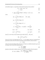
. The model in eq. (56) produces a wide-band
noise, the one in eq. (57) a narrow band, while the model in eq. (58) a mixed character one.
Spectral density characteristics of K

n
(s) and K
d
(s)) are presented in Fig. 3.
wide band mixed narrow band
10
−2
10
−1
10
0
10
1
10
2
10
3
0
0.1
0.2
0.3
0.4
0.5
0.6
0.7
0.8
0.9
1
Magnitude (abs)
|K

c
(jω)|
S
d
(ω)
S
n
(ω)
f
h
Spectral density S(ω); σ
n
=1
Frequency (rad/sec)
h
10
−2
10
−1
10
0
10
1
10
2
10
3
0
0.1
0.2

0.3
0.4
0.5
0.6
0.7
0.8
0.9
1
Magnitude (abs)
|K
c
(jω)|
S
d
(ω)
S
n
(ω)
f
h
Spectral density S(ω); σ
n
=1
Frequency (rad/sec)
h
10
−2
10
−1
10

0
10
1
10
2
10
3
0
0.1
0.2
0.3
0.4
0.5
0.6
0.7
0.8
0.9
1
Magnitude (abs)
|K
c
(jω)|
S
d
(ω)
S
n
(ω)
f
h

Spectral density S(ω); σ
n
=1
Frequency (rad/sec)
h
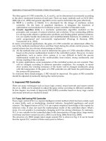
Fig. 3. Spectral density for std {n(t)} = 1.0
4.1 Open-loop results
The effect of Butterworth filter compared with continuous-time Kalman filter in the pure sig-
nal processing context is presented in Fig. 4a - b for a wide-band noise. In Fig. 4a it is clearly
seen, that for small level of noise the only result is that filtration error increases with increas-
ing sampling period h. This is due to the signal deformation caused by filtering. At high noise
Sampled-Data PID Control and Anti-aliasing Filters 135
3.2.2 Discrete-time Kalman filter
Simple instantaneous sampling with sampling period h consists in taking the values of the
sampled signal at discrete time instants t
i
= ih,i = 0, 1, . . Available measurements z
i
are
expressed as
z
i
= y
2
(t
i
). (41)
The problem defined by measurement equation z
i
= z(ih) and state equation (1) is equivalent

to the following discrete-time system:
x
i+1
= F x
i
+ gu
i
+ w
i
, (42)
z
i
= d

x
i
, (43)
where:
F
(τ) = e
A
A
Aτ
, F = F (h), (44)
g
(τ) =
τ

0
e

A
A
Aν
bdν, g = g(h) (45)
and w
i
is a zero mean vector Gaussian noise with E {w
i
w

i
} = W , and
W
=
h

0
e
A
A
As
CC

e
A
A
A

s
ds. (46)

Vectors x
0
and w
i
are independent for all i ≥ 0.
The limiting Kalman filter, (Anderson & Moore, 1979), that provides
( ˆx
i|i
= E [x
i
|z
i
]) for the
discrete-time system in (42)-(43) as i
→ ∞ has the form:
ˆx
i+1|i+1
= ˆx
i+1|i
+ k
f
(z
i+1
−d

ˆx
i+1|i
), (47)
ˆx
i+1|i

= F ˆx
i|i
+ gu
i
, x
0|−1
= 0, (48)
where
k
f
=
Σd
d

Σd
, Σ
= W + F

Σ −
Σdd

Σ

d

Σd

F

. (49)

3.2.3 MV LQG Control System Assessment
Output and control variances for systems with continuous-time filters can be expressed by
following formulae:
σ
2
y
= var{y
i
} = d

0
V
o
d
0
, (50)
σ
2
u
= var{u
i
} = k

x
V
f
k
x
, (51)
where V

o
, V
f
, end V
f o
are submatrices of matrix V
V
= E

x
i
ˆx
i|i


x

i
ˆx

i|i


=

V
o
V
o f
V

f o
V
f

(52)
which is a solution of the following matrix Lyapunov equation:
V
= ΦV Φ

+ ΩW Ω

, (53)
with:
Λ
= (I −k
f
d

)(F + gk

x
), Ψ = (Λ + k
f
d

gk

x
),
Φ

=

F gk

x
k
f
d

F Ψ

, Ω
=

I
k
f
d


.
4. Examples
We will study the properties of control systems for a plant having control path
K
c
(s) =
1
(1 + 0.5s)
2
, (54)

with disturbance modeled by:
K
d
(s) =
k
d
(1 + T
d
s)
2
, (55)
with T
d
= 2 and k
d
chosen such, that var d(t) = 1. For the noise model in Fig.2 we use three
different transfer functions
K
1
n
(s) =
k
1
n
T
2
n
s
2
+ 2ζ

n
T
n
s + 1
, T
n
= 0.05, ζ
n
= 1 (56)
K
2
n
(s) =
k
2
n
T
2
n
s
2
+ 2ζ
n
T
n
s + 1
, T
n
= 0.05, ζ
n

= 0.05 (57)
K
3
n
(s) = k
3
n
·(K
1
n
(s) + K
2
n
(s)) (58)
with k
i
n
, i = 1, 2, 3 chosen such that var n(t) = σ
2
n
. The model in eq. (56) produces a wide-band
noise, the one in eq. (57) a narrow band, while the model in eq. (58) a mixed character one.
Spectral density characteristics of K
n
(s) and K
d
(s)) are presented in Fig. 3.
wide band mixed narrow band
10
−2

10
−1
10
0
10
1
10
2
10
3
0
0.1
0.2
0.3
0.4
0.5
0.6
0.7
0.8
0.9
1
Magnitude (abs)
|K
c
(jω)|
S
d
(ω)
S
n

(ω)
f
h
Spectral density S(ω); σ
n
=1
Frequency (rad/sec)
h
10
−2
10
−1
10
0
10
1
10
2
10
3
0
0.1
0.2
0.3
0.4
0.5
0.6
0.7
0.8
0.9

1
Magnitude (abs)
|K
c
(jω)|
S
d
(ω)
S
n
(ω)
f
h
Spectral density S(ω); σ
n
=1
Frequency (rad/sec)
h
10
−2
10
−1
10
0
10
1
10
2
10
3

0
0.1
0.2
0.3
0.4
0.5
0.6
0.7
0.8
0.9
1
Magnitude (abs)
|K
c
(jω)|
S
d
(ω)
S
n
(ω)
f
h
Spectral density S(ω); σ
n
=1
Frequency (rad/sec)
h
Fig. 3. Spectral density for std {n(t)} = 1.0
4.1 Open-loop results

The effect of Butterworth filter compared with continuous-time Kalman filter in the pure sig-
nal processing context is presented in Fig. 4a - b for a wide-band noise. In Fig. 4a it is clearly
seen, that for small level of noise the only result is that filtration error increases with increas-
ing sampling period h. This is due to the signal deformation caused by filtering. At high noise
PID Control, Implementation and Tuning136
levels there are two effects: decreasing influence of noise with increasing sampling period
accompanied by increasing deformation of the useful signal. This situation becomes greatly
improved when Butterworth filter is followed by a discrete-time Kalman filter of (47)-(48), see
Fig. 4b. In this figure we have std
(∆d
∗
) = lim
i→∞
std {∆d
∗
(i)}, where ∆d
∗
(i) is the difference be-
tween actual value d
i
and a sample s
i
, and std (∆s) = lim
i→∞
std {∆s(i)}, where ∆d(i) = d
i
−
ˆ
d
i|i

is the difference between d
i
and its estimate
ˆ
d
i|i
produced by the discrete-time Kalman filter
These phenomena will play important role in the control context in closed loop.
Butterworth Butterworth with DT Kalman
0 0.2 0.4 0.6 0.8 1
0
0.2
0.4
0.6
0.8
1
h
std{∆d*}
std{n(t)}=0.01; CT(K,η)
std{n(t)}=0.01; CT(B)
std{n(t)}=0.1; CT(K,η)
std{n(t)}=0.1; CT(B)
std{n(t)}=0.5; CT(K,η)
std{n(t)}=0.5; CT(B)
std{n(t)}=1; CT(K,η)
std{n(t)}=1; CT(B)
0 0.2 0.4 0.6 0.8 1
0
0.2
0.4

0.6
0.8
1
h
std{∆d*},std{∆d}
std{n(t)}=0.01; CT(K,η)
std{n(t)}=0.01; CT(B)+DT(η)
std{n(t)}=0.1; CT(K,η)
std{n(t)}=0.1; CT(B)+DT(η)
std{n(t)}=0.5; CT(K,η)
std{n(t)}=0.5; CT(B)+DT(η)
std{n(t)}=1; CT(K,η)
std{n(t)}=1; CT(B)+DT(η)
Fig. 4. Wide-band noise filtering results: CT Butterworth filter and CT Butterworth with DT
Kalman compared with CT Kalman filter
Butterworth Butterworth with DT Kalman
0 0.2 0.4 0.6 0.8 1
0
0.2
0.4
0.6
0.8
1
h
std{∆d*}
std{n(t)}=0.01; CT(K,η)
std{n(t)}=0.01; CT(B)
std{n(t)}=0.1; CT(K,η)
std{n(t)}=0.1; CT(B)
std{n(t)}=0.5; CT(K,η)

std{n(t)}=0.5; CT(B)
std{n(t)}=1; CT(K,η)
std{n(t)}=1; CT(B)
0 0.2 0.4 0.6 0.8 1
0
0.2
0.4
0.6
0.8
1
h
std{∆d*},std{∆d}
std{n(t)}=0.01; CT(K,η)
std{n(t)}=0.01; CT(B)+DT(η)
std{n(t)}=0.1; CT(K,η)
std{n(t)}=0.1; CT(B)+DT(η)
std{n(t)}=0.5; CT(K,η)
std{n(t)}=0.5; CT(B)+DT(η)
std{n(t)}=1; CT(K,η)
std{n(t)}=1; CT(B)+DT(η)
Fig. 5. Narrow-band noise filtering results: CT Butterworth filter and CT Butterworth with
DT Kalman compared with CT Kalman filter
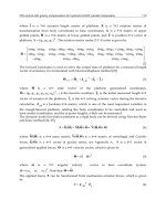
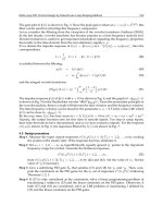
4.2 Closed-loop results
The results for PID QDR, optimal PID and LQG controlled systems are presented in figure
Fig. 6 as functions of the sampling period h. The main conclusion is that all control systems
0 0.1 0.2 0.3 0.4 0.5
0
0.5
1
h

std{y
i
}
PID(QDR); std{n}=0
0 0.1 0.2 0.3 0.4 0.5
0
2
4
h
std{u
i
}
PID
PID; CT(B)
PID; CT(K)−η
0 0.1 0.2 0.3 0.4 0.5
0
0.5
1
h
std{y
i
}
PID(opt); std{n}=0
0 0.1 0.2 0.3 0.4 0.5
0
2
4
h
std{u

i
}
PID
PID; CT(B)
PID; CT(K)−η
0 0.1 0.2 0.3 0.4 0.5
0
0.5
1
h
std{y
i
}
LQG; std{n}=0
0 0.1 0.2 0.3 0.4 0.5
0
2
4
h
std{u
i
}
LQG
LQG; CT(B)
LQG; CT(K)−η
0 0.1 0.2 0.3 0.4 0.5
0
0.5
1
h

std{y
i
}
PID(QDR); std{n}=0.1
0 0.1 0.2 0.3 0.4 0.5
0
2
4
h
std{u
i
}
PID
PID; CT(B)
PID; CT(K)−η
0 0.1 0.2 0.3 0.4 0.5
0
0.5
1
h
std{y
i
}
PID(opt); std{n}=0.1
0 0.1 0.2 0.3 0.4 0.5
0
2
4
h
std{u

i
}
PID
PID; CT(B)
PID; CT(K)−η
0 0.1 0.2 0.3 0.4 0.5
0
0.5
1
h
std{y
i
}
LQG; std{n}=0.1
0 0.1 0.2 0.3 0.4 0.5
0
2
4
h
std{u
i
}
LQG
LQG; CT(B)
LQG; CT(K)−η
0 0.1 0.2 0.3 0.4 0.5
0
0.5
1
h

std{y
i
}
PID(QDR); std{n}=1
0 0.1 0.2 0.3 0.4 0.5
0
5
10
h
std{u
i
}
PID
PID; CT(B)
PID; CT(K)−η
0 0.1 0.2 0.3 0.4 0.5
0
0.5
1
h
std{y
i
}
PID(opt); std{n}=1
0 0.1 0.2 0.3 0.4 0.5
0
5
10
h
std{u

i
}
PID
PID; CT(B)
PID; CT(K)−η
0 0.1 0.2 0.3 0.4 0.5
0
0.5
1
h
std{y
i
}
LQG; std{n}=1
0 0.1 0.2 0.3 0.4 0.5
0
10
20
30
h
std{u
i
}
LQG
LQG; CT(B)
LQG; CT(K)−η
Fig. 6. Control errors and control efforts as functions of h for various noise magnitudes
behave worse when the anti-aliasing filter is used in the noiseless case. This is also true in the
case of small noise level and PID controllers.
In contrast to the LQG control, the continuous-time Kalman filter does not help either. Very

small improvement is attained in MV LQG system at very high noise level and longer sam-
pling periods. The characteristic feature of MV LQG is that the control magnitudes do not
depend on the type of filter used.
The improvement in terms of output variance is better visible in the case of PID controllers.
Systems with Kalman filter behave then better in wide range of sampling instants.
Rather large improvement is seen, however, in terms of control signal magnitudes. It does not
depend practically on sampling period in the case of CT Kalman filter, and tends to it with
increasing sampling period in the case of Butterworth filter.
Selected results for PID and LQG controllers with parameters collected in Table 2 are illus-
trated in Fig.7 on the plane std{u}–std{y} for h
= 0.2. It is readily seen that analog filtering
makes restricted sense only for PID controllers with QDR tuning and high noise level. Un-
fortunately the quality of control remains then very poor, even if the continuous-time Kalman
filter is applied as analog filter. Application of optimally tuned PID controllers leads to an
even more surprising result: from figure Fig.7 it is seen that even at large noise level very
good results close to the LQG benchmark can be obtained without any analog filter.
In Fig.7the results are plotted on the plane std{u}–std{y} for various values of h, showing
again that the use of anti-aliasing filter makes no sense, and that the quality of disturbance
attenuation of optimally tuned PID controllers is very similar to that of MV LQG controller.
Unfortunately, Nyquist plots of a series connection of the plant and the controller depicted in
Fig.8 show that PID systems are less robust than the MV LQG ones. Moreover, the usage of
anti-aliasing filters makes this even worse.
Sampled-Data PID Control and Anti-aliasing Filters 137
levels there are two effects: decreasing influence of noise with increasing sampling period
accompanied by increasing deformation of the useful signal. This situation becomes greatly
improved when Butterworth filter is followed by a discrete-time Kalman filter of (47)-(48), see
Fig. 4b. In this figure we have std
(∆d
∗
) = lim

i→∞
std {∆d
∗
(i)}, where ∆d
∗
(i) is the difference be-
tween actual value d
i
and a sample s
i
, and std (∆s) = lim
i→∞
std {∆s(i)}, where ∆d(i) = d
i
−
ˆ
d
i|i
is the difference between d
i
and its estimate
ˆ
d
i|i
produced by the discrete-time Kalman filter
These phenomena will play important role in the control context in closed loop.
Butterworth Butterworth with DT Kalman
0 0.2 0.4 0.6 0.8 1
0
0.2

0.4
0.6
0.8
1
h
std{∆d*}
std{n(t)}=0.01; CT(K,η)
std{n(t)}=0.01; CT(B)
std{n(t)}=0.1; CT(K,η)
std{n(t)}=0.1; CT(B)
std{n(t)}=0.5; CT(K,η)
std{n(t)}=0.5; CT(B)
std{n(t)}=1; CT(K,η)
std{n(t)}=1; CT(B)
0 0.2 0.4 0.6 0.8 1
0
0.2
0.4
0.6
0.8
1
h
std{∆d*},std{∆d}
std{n(t)}=0.01; CT(K,η)
std{n(t)}=0.01; CT(B)+DT(η)
std{n(t)}=0.1; CT(K,η)
std{n(t)}=0.1; CT(B)+DT(η)
std{n(t)}=0.5; CT(K,η)
std{n(t)}=0.5; CT(B)+DT(η)
std{n(t)}=1; CT(K,η)

std{n(t)}=1; CT(B)+DT(η)
Fig. 4. Wide-band noise filtering results: CT Butterworth filter and CT Butterworth with DT
Kalman compared with CT Kalman filter
Butterworth Butterworth with DT Kalman
0 0.2 0.4 0.6 0.8 1
0
0.2
0.4
0.6
0.8
1
h
std{∆d*}
std{n(t)}=0.01; CT(K,η)
std{n(t)}=0.01; CT(B)
std{n(t)}=0.1; CT(K,η)
std{n(t)}=0.1; CT(B)
std{n(t)}=0.5; CT(K,η)
std{n(t)}=0.5; CT(B)
std{n(t)}=1; CT(K,η)
std{n(t)}=1; CT(B)
0 0.2 0.4 0.6 0.8 1
0
0.2
0.4
0.6
0.8
1
h
std{∆d*},std{∆d}

std{n(t)}=0.01; CT(K,η)
std{n(t)}=0.01; CT(B)+DT(η)
std{n(t)}=0.1; CT(K,η)
std{n(t)}=0.1; CT(B)+DT(η)
std{n(t)}=0.5; CT(K,η)
std{n(t)}=0.5; CT(B)+DT(η)
std{n(t)}=1; CT(K,η)
std{n(t)}=1; CT(B)+DT(η)
Fig. 5. Narrow-band noise filtering results: CT Butterworth filter and CT Butterworth with
DT Kalman compared with CT Kalman filter
4.2 Closed-loop results
The results for PID QDR, optimal PID and LQG controlled systems are presented in figure
Fig. 6 as functions of the sampling period h. The main conclusion is that all control systems
0 0.1 0.2 0.3 0.4 0.5
0
0.5
1
h
std{y
i
}
PID(QDR); std{n}=0
0 0.1 0.2 0.3 0.4 0.5
0
2
4
h
std{u
i
}

PID
PID; CT(B)
PID; CT(K)−η
0 0.1 0.2 0.3 0.4 0.5
0
0.5
1
h
std{y
i
}
PID(opt); std{n}=0
0 0.1 0.2 0.3 0.4 0.5
0
2
4
h
std{u
i
}
PID
PID; CT(B)
PID; CT(K)−η
0 0.1 0.2 0.3 0.4 0.5
0
0.5
1
h
std{y
i

}
LQG; std{n}=0
0 0.1 0.2 0.3 0.4 0.5
0
2
4
h
std{u
i
}
LQG
LQG; CT(B)
LQG; CT(K)−η
0 0.1 0.2 0.3 0.4 0.5
0
0.5
1
h
std{y
i
}
PID(QDR); std{n}=0.1
0 0.1 0.2 0.3 0.4 0.5
0
2
4
h
std{u
i
}

PID
PID; CT(B)
PID; CT(K)−η
0 0.1 0.2 0.3 0.4 0.5
0
0.5
1
h
std{y
i
}
PID(opt); std{n}=0.1
0 0.1 0.2 0.3 0.4 0.5
0
2
4
h
std{u
i
}
PID
PID; CT(B)
PID; CT(K)−η
0 0.1 0.2 0.3 0.4 0.5
0
0.5
1
h
std{y
i

}
LQG; std{n}=0.1
0 0.1 0.2 0.3 0.4 0.5
0
2
4
h
std{u
i
}
LQG
LQG; CT(B)
LQG; CT(K)−η
0 0.1 0.2 0.3 0.4 0.5
0
0.5
1
h
std{y
i
}
PID(QDR); std{n}=1
0 0.1 0.2 0.3 0.4 0.5
0
5
10
h
std{u
i
}

PID
PID; CT(B)
PID; CT(K)−η
0 0.1 0.2 0.3 0.4 0.5
0
0.5
1
h
std{y
i
}
PID(opt); std{n}=1
0 0.1 0.2 0.3 0.4 0.5
0
5
10
h
std{u
i
}
PID
PID; CT(B)
PID; CT(K)−η
0 0.1 0.2 0.3 0.4 0.5
0
0.5
1
h
std{y
i

}
LQG; std{n}=1
0 0.1 0.2 0.3 0.4 0.5
0
10
20
30
h
std{u
i
}
LQG
LQG; CT(B)
LQG; CT(K)−η
Fig. 6. Control errors and control efforts as functions of h for various noise magnitudes
behave worse when the anti-aliasing filter is used in the noiseless case. This is also true in the
case of small noise level and PID controllers.
In contrast to the LQG control, the continuous-time Kalman filter does not help either. Very
small improvement is attained in MV LQG system at very high noise level and longer sam-
pling periods. The characteristic feature of MV LQG is that the control magnitudes do not
depend on the type of filter used.
The improvement in terms of output variance is better visible in the case of PID controllers.
Systems with Kalman filter behave then better in wide range of sampling instants.
Rather large improvement is seen, however, in terms of control signal magnitudes. It does not
depend practically on sampling period in the case of CT Kalman filter, and tends to it with
increasing sampling period in the case of Butterworth filter.
Selected results for PID and LQG controllers with parameters collected in Table 2 are illus-
trated in Fig.7 on the plane std{u}–std{y} for h
= 0.2. It is readily seen that analog filtering
makes restricted sense only for PID controllers with QDR tuning and high noise level. Un-

fortunately the quality of control remains then very poor, even if the continuous-time Kalman
filter is applied as analog filter. Application of optimally tuned PID controllers leads to an
even more surprising result: from figure Fig.7 it is seen that even at large noise level very
good results close to the LQG benchmark can be obtained without any analog filter.
In Fig.7the results are plotted on the plane std{u}–std{y} for various values of h, showing
again that the use of anti-aliasing filter makes no sense, and that the quality of disturbance
attenuation of optimally tuned PID controllers is very similar to that of MV LQG controller.
Unfortunately, Nyquist plots of a series connection of the plant and the controller depicted in
Fig.8 show that PID systems are less robust than the MV LQG ones. Moreover, the usage of
anti-aliasing filters makes this even worse.
PID Control, Implementation and Tuning138
QDR std{y
i
} OPTIMAL std {y
i
}
PID
k
P
= 2.8146
T
I
= 0.7045
T
D
= 0.1761
0.78
k
P
= 0.9383

T
I
= 0.9647
T
D
= 0.2199
0.50
PID;B
k
P
= 2.2328
T
I
= 0.8843
T
D
= 0.2211
0.71
k
P
= 0.9293
T
I
= 0.9486
T
D
= 0.2427
0.50
PID;K
k

P
= 1.8621
T
I
= 1.6319
T
D
= 0.4080
0.55
k
P
= 1.4118
T
I
= 1.5648
T
D
= 0.6619
0.53
Table 2. QDR PID & Optimal PID controller settings for std
{n} = 1 and h = 0.2
0 2 4 6 8
0
0.2
0.4
0.6
0.8
1
1.2
PID(QDR),

σ
n
=0
PID(QDR);B
PID(QDR);K
PID, σ
n
=0
PID;B
PID;K
PID(QDR), σ
n
=1
PID(QDR);B
PID(QDR);K
PID, σ
n
=1
PID;B
PID;K
std{u
i
}
std{y
i
}
PID(QDR) & PID; h=0.2
PID(QDR), σ
n
=0

PID(QDR);B
PID(QDR);K
PID, σ
n
=0
PID;B
PID;K
PID(QDR), σ
n
=1
PID(QDR);B
PID(QDR);K
PID, σ
n
=1
PID;B
PID;K
Fig. 7. PID QDR & optimal PID controller results, for h = 0.2 with std {n(t)} = 0 and
std
{n(t)} = 1
−1 −0.5 0 0.5
−2.5
−2
−1.5
−1
−0.5
0
0.5
1
1.5

2
2.5
(−1,0j)
PID
PID;CT(B)
PID;CT(K)−η
PID(QDR); std{n(t)}=1; h=0.5
Frequency (rad/sec)
Magnitude (abs)
−1 −0.5 0 0.5
−2.5
−2
−1.5
−1
−0.5
0
0.5
1
1.5
2
2.5
(−1,0j)
PID
PID;CT(B)
PID;CT(K)−η
PID(opt); std{n(t)}=1; h=0.5
Frequency (rad/sec)
Magnitude (abs)
−1 −0.5 0 0.5
−2.5

−2
−1.5
−1
−0.5
0
0.5
1
1.5
2
2.5
(−1,0j)
LQG
LQG;CT(B)
LQG;CT(K)−η
LQG; std{n(t)}=1; h=0.5
Frequency (rad/sec)
Magnitude (abs)
Fig. 8. Nyquist plots and robustness of various control systems
Influence of sampling period and noise character is further studied in figures Fig.9 - Fig.14
no filter Kalman Butterworth
0 5 10 15 20
0
0.2
0.4
0.6
0.8
1
std{u
i
}

std{y
i
}
PID(QDR),PID(opt),LQG&LQG(λ=0.001); σ
n
=0.01
PID(QDR)
PID(opt)
LQG λ=0
LQG λ=0.001
0 5 10 15 20
0
0.2
0.4
0.6
0.8
1
std{u
i
}
std{y
i
}
PID(QDR),PID(opt)&LQG ; σ
n
=0.01; CT(K)−η
PID(QDR)
PID(opt)
LQG λ=0
0 5 10 15 20

0
0.2
0.4
0.6
0.8
1
std{u
i
}
std{y
i
}
PID(QDR),PID(opt)&LQG ; σ
n
=0.01; CT(B)
PID(QDR)
PID(opt)
LQG λ=0
Fig. 9. Negligible noise level results as functions of h, std {n
i
} = 0.01
no filter Kalman Butterworth
0 5 10 15 20
0
0.2
0.4
0.6
0.8
1
std{u

i
}
std{y
i
}
PID(QDR),PID(opt),LQG&LQG(λ=0.001); σ
n
=0.5
PID(QDR)
PID(opt)
LQG λ=0
LQG λ=0.001
0 5 10 15 20
0
0.2
0.4
0.6
0.8
1
std{u
i
}
std{y
i
}
PID(QDR),PID(opt)&LQG ; σ
n
=0.5; CT(K)−η
PID(QDR)
PID(opt)

LQG λ=0
0 5 10 15 20
0
0.2
0.4
0.6
0.8
1
std{u
i
}
std{y
i
}
PID(QDR),PID(opt)&LQG ; σ
n
=0.5; CT(B)
PID(QDR)
PID(opt)
LQG λ=0
Fig. 10. Wide-band noise results for various controllers and filters as functions of h
no filter Kalman Butterworth
0 5 10 15 20
0
0.2
0.4
0.6
0.8
1
std{u

i
}
std{y
i
}
PID(QDR),PID(opt),LQG&LQG(λ=0.001); σ
n
=0.5
PID(QDR)
PID(opt)
LQG λ=0
LQG λ=0.001
0 5 10 15 20
0
0.2
0.4
0.6
0.8
1
std{u
i
}
std{y
i
}
PID(QDR),PID(opt)&LQG ; σ
n
=0.5; CT(K)−η
PID(QDR)
PID(opt)

LQG λ=0
0 5 10 15 20
0
0.2
0.4
0.6
0.8
1
std{u
i
}
std{y
i
}
PID(QDR),PID(opt)&LQG ; σ
n
=0.5; CT(B)
PID(QDR)
PID(opt)
LQG λ=0
Fig. 11. Mixed-band noise results for various controllers and filters as functions of h
no filter Kalman Butterworth
0 5 10 15 20
0
0.2
0.4
0.6
0.8
1
std{u

i
}
std{y
i
}
PID(QDR),PID(opt),LQG&LQG(λ=0.001); σ
n
=0.5
PID(QDR)
PID(opt)
LQG λ=0
LQG λ=0.001
0 5 10 15 20
0
0.2
0.4
0.6
0.8
1
std{u
i
}
std{y
i
}
PID(QDR),PID(opt)&LQG ; σ
n
=0.5; CT(K)−η
PID(QDR)
PID(opt)

LQG λ=0
0 5 10 15 20
0
0.2
0.4
0.6
0.8
1
std{u
i
}
std{y
i
}
PID(QDR),PID(opt)&LQG ; σ
n
=0.5; CT(B)
PID(QDR)
PID(opt)
LQG λ=0
Fig. 12. Narrow-band noise results for various controllers and filters as functions of h
Sampled-Data PID Control and Anti-aliasing Filters 139
QDR std{y
i
} OPTIMAL std {y
i
}
PID
k
P

= 2.8146
T
I
= 0.7045
T
D
= 0.1761
0.78
k
P
= 0.9383
T
I
= 0.9647
T
D
= 0.2199
0.50
PID;B
k
P
= 2.2328
T
I
= 0.8843
T
D
= 0.2211
0.71
k

P
= 0.9293
T
I
= 0.9486
T
D
= 0.2427
0.50
PID;K
k
P
= 1.8621
T
I
= 1.6319
T
D
= 0.4080
0.55
k
P
= 1.4118
T
I
= 1.5648
T
D
= 0.6619
0.53

Table 2. QDR PID & Optimal PID controller settings for std
{n} = 1 and h = 0.2
0 2 4 6 8
0
0.2
0.4
0.6
0.8
1
1.2
PID(QDR),
σ
n
=0
PID(QDR);B
PID(QDR);K
PID, σ
n
=0
PID;B
PID;K
PID(QDR), σ
n
=1
PID(QDR);B
PID(QDR);K
PID, σ
n
=1
PID;B

PID;K
std{u
i
}
std{y
i
}
PID(QDR) & PID; h=0.2
PID(QDR), σ
n
=0
PID(QDR);B
PID(QDR);K
PID, σ
n
=0
PID;B
PID;K
PID(QDR), σ
n
=1
PID(QDR);B
PID(QDR);K
PID, σ
n
=1
PID;B
PID;K
Fig. 7. PID QDR & optimal PID controller results, for h = 0.2 with std {n(t)} = 0 and
std

{n(t)} = 1
−1 −0.5 0 0.5
−2.5
−2
−1.5
−1
−0.5
0
0.5
1
1.5
2
2.5
(−1,0j)
PID
PID;CT(B)
PID;CT(K)−η
PID(QDR); std{n(t)}=1; h=0.5
Frequency (rad/sec)
Magnitude (abs)
−1 −0.5 0 0.5
−2.5
−2
−1.5
−1
−0.5
0
0.5
1
1.5

2
2.5
(−1,0j)
PID
PID;CT(B)
PID;CT(K)−η
PID(opt); std{n(t)}=1; h=0.5
Frequency (rad/sec)
Magnitude (abs)
−1 −0.5 0 0.5
−2.5
−2
−1.5
−1
−0.5
0
0.5
1
1.5
2
2.5
(−1,0j)
LQG
LQG;CT(B)
LQG;CT(K)−η
LQG; std{n(t)}=1; h=0.5
Frequency (rad/sec)
Magnitude (abs)
Fig. 8. Nyquist plots and robustness of various control systems
Influence of sampling period and noise character is further studied in figures Fig.9 - Fig.14

no filter Kalman Butterworth
0 5 10 15 20
0
0.2
0.4
0.6
0.8
1
std{u
i
}
std{y
i
}
PID(QDR),PID(opt),LQG&LQG(λ=0.001); σ
n
=0.01
PID(QDR)
PID(opt)
LQG λ=0
LQG λ=0.001
0 5 10 15 20
0
0.2
0.4
0.6
0.8
1
std{u
i

}
std{y
i
}
PID(QDR),PID(opt)&LQG ; σ
n
=0.01; CT(K)−η
PID(QDR)
PID(opt)
LQG λ=0
0 5 10 15 20
0
0.2
0.4
0.6
0.8
1
std{u
i
}
std{y
i
}
PID(QDR),PID(opt)&LQG ; σ
n
=0.01; CT(B)
PID(QDR)
PID(opt)
LQG λ=0
Fig. 9. Negligible noise level results as functions of h, std {n

i
} = 0.01
no filter Kalman Butterworth
0 5 10 15 20
0
0.2
0.4
0.6
0.8
1
std{u
i
}
std{y
i
}
PID(QDR),PID(opt),LQG&LQG(λ=0.001); σ
n
=0.5
PID(QDR)
PID(opt)
LQG λ=0
LQG λ=0.001
0 5 10 15 20
0
0.2
0.4
0.6
0.8
1

std{u
i
}
std{y
i
}
PID(QDR),PID(opt)&LQG ; σ
n
=0.5; CT(K)−η
PID(QDR)
PID(opt)
LQG λ=0
0 5 10 15 20
0
0.2
0.4
0.6
0.8
1
std{u
i
}
std{y
i
}
PID(QDR),PID(opt)&LQG ; σ
n
=0.5; CT(B)
PID(QDR)
PID(opt)

LQG λ=0
Fig. 10. Wide-band noise results for various controllers and filters as functions of h
no filter Kalman Butterworth
0 5 10 15 20
0
0.2
0.4
0.6
0.8
1
std{u
i
}
std{y
i
}
PID(QDR),PID(opt),LQG&LQG(λ=0.001); σ
n
=0.5
PID(QDR)
PID(opt)
LQG λ=0
LQG λ=0.001
0 5 10 15 20
0
0.2
0.4
0.6
0.8
1

std{u
i
}
std{y
i
}
PID(QDR),PID(opt)&LQG ; σ
n
=0.5; CT(K)−η
PID(QDR)
PID(opt)
LQG λ=0
0 5 10 15 20
0
0.2
0.4
0.6
0.8
1
std{u
i
}
std{y
i
}
PID(QDR),PID(opt)&LQG ; σ
n
=0.5; CT(B)
PID(QDR)
PID(opt)

LQG λ=0
Fig. 11. Mixed-band noise results for various controllers and filters as functions of h
no filter Kalman Butterworth
0 5 10 15 20
0
0.2
0.4
0.6
0.8
1
std{u
i
}
std{y
i
}
PID(QDR),PID(opt),LQG&LQG(λ=0.001); σ
n
=0.5
PID(QDR)
PID(opt)
LQG λ=0
LQG λ=0.001
0 5 10 15 20
0
0.2
0.4
0.6
0.8
1

std{u
i
}
std{y
i
}
PID(QDR),PID(opt)&LQG ; σ
n
=0.5; CT(K)−η
PID(QDR)
PID(opt)
LQG λ=0
0 5 10 15 20
0
0.2
0.4
0.6
0.8
1
std{u
i
}
std{y
i
}
PID(QDR),PID(opt)&LQG ; σ
n
=0.5; CT(B)
PID(QDR)
PID(opt)

LQG λ=0
Fig. 12. Narrow-band noise results for various controllers and filters as functions of h
PID Control, Implementation and Tuning140
no filter Kalman Butterworth
0 5 10 15 20 25 30
−2
−1
0
1
2
PID(QDR); h=0.05; std{n}=0.5
y
2
(t)
y
f
(t)
y(t)
2σ
y
0 5 10 15 20 25 30
−10
−5
0
5
10
t[s]
u
i
2σ

u
0 5 10 15 20 25 30
−2
−1
0
1
2
PID(QDR), CTR(K); h=0.05; std{n}=0.5
y
2
(t)
y
f
(t)
y(t)
2σ
y
0 5 10 15 20 25 30
−10
−5
0
5
10
t[s]
u
i
2σ
u
0 5 10 15 20 25 30
−2

−1
0
1
2
PID(QDR), CTR(B); h=0.05; std{n}=0.5
y
2
(t)
y
f
(t)
y(t)
2σ
y
0 5 10 15 20 25 30
−10
−5
0
5
10
t[s]
u
i
2σ
u
0 5 10 15 20 25 30
−2
−1
0
1

2
PID(opt); h=0.05; std{n}=0.5
y
2
(t)
y
f
(t)
y(t)
2σ
y
0 5 10 15 20 25 30
−10
−5
0
5
10
t[s]
u
i
2σ
u
0 5 10 15 20 25 30
−2
−1
0
1
2
PID(opt), CTR(K); h=0.05; std{n}=0.5
y

2
(t)
y
f
(t)
y(t)
2σ
y
0 5 10 15 20 25 30
−10
−5
0
5
10
t[s]
u
i
2σ
u
0 5 10 15 20 25 30
−2
−1
0
1
2
PID(opt), CTR(B); h=0.05; std{n}=0.5
y
2
(t)
y

f
(t)
y(t)
2σ
y
0 5 10 15 20 25 30
−10
−5
0
5
10
t[s]
u
i
2σ
u
0 5 10 15 20 25 30
−2
−1
0
1
2
LQG, h=0.05; std{n}=0.5
y
2
(t)
y
f
(t)
y(t)

2σ
y
0 5 10 15 20 25 30
−10
−5
0
5
10
t[s]
u
i
2σ
u
0 5 10 15 20 25 30
−2
−1
0
1
2
LQG, CTR(K); h=0.05; std{n}=0.5
y
2
(t)
y
f
(t)
y(t)
2σ
y
0 5 10 15 20 25 30

−10
−5
0
5
10
t[s]
u
i
2σ
u
0 5 10 15 20 25 30
−2
−1
0
1
2
LQG, CTR(B); h=0.05; std{n}=0.5
y
2
(t)
y
f
(t)
y(t)
2σ
y
0 5 10 15 20 25 30
−10
−5
0

5
10
t[s]
u
i
2σ
u
Fig. 13. Wide-band noise: realizations of output and control signals
5. Conclusion
It has been shown that the use of anti-aliasing filters is not justified in sampled-data MV LQG
and PID control systems with noiseless measurements, or when the level of noise is small.
Certain improvement can be made in the case of PID control systems with QDR and optimal
settings in terms of both, output signal and control signal variance, in the case of large level of
noise. However, continuous-time Kalman filter is then much better in the wide range of sam-
pling periods, while the effect of Butterworth filter becomes better with increasing sampling
period. Unfortunately the usage of any analog filters deteriorates the robustness of control
systems. This makes the claim of uselessness of anti-aliasing filters even stronger.
Optimal tuning of PID controllers that takes the disturbance and noise parameters into ac-
count leads to the results comparable with those of LQG controllers without any analog pre-
filters. (Goodwin et al., 2001)
no filter Kalman Butterworth
0 5 10 15 20 25 30
−2
−1
0
1
2
PID(QDR); h=0.05; std{n}=0.5
y
2

(t)
y
f
(t)
y(t)
2σ
y
0 5 10 15 20 25 30
−10
−5
0
5
10
t[s]
u
i
2σ
u
0 5 10 15 20 25 30
−2
−1
0
1
2
PID(QDR), CTR(K); h=0.05; std{n}=0.5
y
2
(t)
y
f

(t)
y(t)
2σ
y
0 5 10 15 20 25 30
−10
−5
0
5
10
t[s]
u
i
2σ
u
0 5 10 15 20 25 30
−2
−1
0
1
2
PID(QDR), CTR(B); h=0.05; std{n}=0.5
y
2
(t)
y
f
(t)
y(t)
2σ

y
0 5 10 15 20 25 30
−10
−5
0
5
10
t[s]
u
i
2σ
u
0 5 10 15 20 25 30
−2
−1
0
1
2
PID(opt); h=0.05; std{n}=0.5
y
2
(t)
y
f
(t)
y(t)
2σ
y
0 5 10 15 20 25 30
−10

−5
0
5
10
t[s]
u
i
2σ
u
0 5 10 15 20 25 30
−2
−1
0
1
2
PID(opt), CTR(K); h=0.05; std{n}=0.5
y
2
(t)
y
f
(t)
y(t)
2σ
y
0 5 10 15 20 25 30
−10
−5
0
5

10
t[s]
u
i
2σ
u
0 5 10 15 20 25 30
−2
−1
0
1
2
PID(opt), CTR(B); h=0.05; std{n}=0.5
y
2
(t)
y
f
(t)
y(t)
2σ
y
0 5 10 15 20 25 30
−10
−5
0
5
10
t[s]
u

i
2σ
u
0 5 10 15 20 25 30
−2
−1
0
1
2
LQG, h=0.05; std{n}=0.5
y
2
(t)
y
f
(t)
y(t)
2σ
y
0 5 10 15 20 25 30
−10
−5
0
5
10
t[s]
u
i
2σ
u

0 5 10 15 20 25 30
−2
−1
0
1
2
LQG, CTR(K); h=0.05; std{n}=0.5
y
2
(t)
y
f
(t)
y(t)
2σ
y
0 5 10 15 20 25 30
−10
−5
0
5
10
t[s]
u
i
2σ
u
0 5 10 15 20 25 30
−2
−1

0
1
2
LQG, CTR(B); h=0.05; std{n}=0.5
y
2
(t)
y
f
(t)
y(t)
2σ
y
0 5 10 15 20 25 30
−10
−5
0
5
10
t[s]
u
i
2σ
u
Fig. 14. Narrow-band noise: realizations of output and control signals
6. References
Anderson, B.D.O. and Moore, J.B. (1979). Optimal Filtering, Prentice Hall, Inc., Englewood
Cliffs, New Jersey, .
Åström, K. and Wittenmark, B. (1997). Computer–Controlled Systems, Prentice Hall, 1997.
Blachuta, M. J., Grygiel, R. T. (2008a). Averaging sampling: models and properties. Proc. of the

2008 American Control Conference, pp. 3554-3559, Seattle USA, June 2008.
Blachuta, M. J., Grygiel, R. T. (2008b). Sampling of noisy signals: spectral vs anti-aliasing
filters, Proc. of the 2008 IFAC World Congress, pp. 7576-7581, Seul Korea, July 2008.
Blachuta, M. J., Grygiel, R. T. (2009a). On the Effect of Antialiasing Filters on Sampled-Data
PID Control, Proc. of 21th Chinese Conference on Decision and Control, Guilin China,
June 2009.
Blachuta, M. J., Grygiel, R. T. (2009b). Are anti-aliasing filters really necessary for sampled-
data control? Proc. of the 2009 American Control Coference, pp. 3200-3205, St Louis
USA, June 2009.
Sampled-Data PID Control and Anti-aliasing Filters 141
no filter Kalman Butterworth
0 5 10 15 20 25 30
−2
−1
0
1
2
PID(QDR); h=0.05; std{n}=0.5
y
2
(t)
y
f
(t)
y(t)
2σ
y
0 5 10 15 20 25 30
−10
−5

0
5
10
t[s]
u
i
2σ
u
0 5 10 15 20 25 30
−2
−1
0
1
2
PID(QDR), CTR(K); h=0.05; std{n}=0.5
y
2
(t)
y
f
(t)
y(t)
2σ
y
0 5 10 15 20 25 30
−10
−5
0
5
10

t[s]
u
i
2σ
u
0 5 10 15 20 25 30
−2
−1
0
1
2
PID(QDR), CTR(B); h=0.05; std{n}=0.5
y
2
(t)
y
f
(t)
y(t)
2σ
y
0 5 10 15 20 25 30
−10
−5
0
5
10
t[s]
u
i

2σ
u
0 5 10 15 20 25 30
−2
−1
0
1
2
PID(opt); h=0.05; std{n}=0.5
y
2
(t)
y
f
(t)
y(t)
2σ
y
0 5 10 15 20 25 30
−10
−5
0
5
10
t[s]
u
i
2σ
u
0 5 10 15 20 25 30

−2
−1
0
1
2
PID(opt), CTR(K); h=0.05; std{n}=0.5
y
2
(t)
y
f
(t)
y(t)
2σ
y
0 5 10 15 20 25 30
−10
−5
0
5
10
t[s]
u
i
2σ
u
0 5 10 15 20 25 30
−2
−1
0

1
2
PID(opt), CTR(B); h=0.05; std{n}=0.5
y
2
(t)
y
f
(t)
y(t)
2σ
y
0 5 10 15 20 25 30
−10
−5
0
5
10
t[s]
u
i
2σ
u
0 5 10 15 20 25 30
−2
−1
0
1
2
LQG, h=0.05; std{n}=0.5

y
2
(t)
y
f
(t)
y(t)
2σ
y
0 5 10 15 20 25 30
−10
−5
0
5
10
t[s]
u
i
2σ
u
0 5 10 15 20 25 30
−2
−1
0
1
2
LQG, CTR(K); h=0.05; std{n}=0.5
y
2
(t)

y
f
(t)
y(t)
2σ
y
0 5 10 15 20 25 30
−10
−5
0
5
10
t[s]
u
i
2σ
u
0 5 10 15 20 25 30
−2
−1
0
1
2
LQG, CTR(B); h=0.05; std{n}=0.5
y
2
(t)
y
f
(t)

y(t)
2σ
y
0 5 10 15 20 25 30
−10
−5
0
5
10
t[s]
u
i
2σ
u
Fig. 13. Wide-band noise: realizations of output and control signals
5. Conclusion
It has been shown that the use of anti-aliasing filters is not justified in sampled-data MV LQG
and PID control systems with noiseless measurements, or when the level of noise is small.
Certain improvement can be made in the case of PID control systems with QDR and optimal
settings in terms of both, output signal and control signal variance, in the case of large level of
noise. However, continuous-time Kalman filter is then much better in the wide range of sam-
pling periods, while the effect of Butterworth filter becomes better with increasing sampling
period. Unfortunately the usage of any analog filters deteriorates the robustness of control
systems. This makes the claim of uselessness of anti-aliasing filters even stronger.
Optimal tuning of PID controllers that takes the disturbance and noise parameters into ac-
count leads to the results comparable with those of LQG controllers without any analog pre-
filters. (Goodwin et al., 2001)
no filter Kalman Butterworth
0 5 10 15 20 25 30
−2

−1
0
1
2
PID(QDR); h=0.05; std{n}=0.5
y
2
(t)
y
f
(t)
y(t)
2σ
y
0 5 10 15 20 25 30
−10
−5
0
5
10
t[s]
u
i
2σ
u
0 5 10 15 20 25 30
−2
−1
0
1

2
PID(QDR), CTR(K); h=0.05; std{n}=0.5
y
2
(t)
y
f
(t)
y(t)
2σ
y
0 5 10 15 20 25 30
−10
−5
0
5
10
t[s]
u
i
2σ
u
0 5 10 15 20 25 30
−2
−1
0
1
2
PID(QDR), CTR(B); h=0.05; std{n}=0.5
y

2
(t)
y
f
(t)
y(t)
2σ
y
0 5 10 15 20 25 30
−10
−5
0
5
10
t[s]
u
i
2σ
u
0 5 10 15 20 25 30
−2
−1
0
1
2
PID(opt); h=0.05; std{n}=0.5
y
2
(t)
y

f
(t)
y(t)
2σ
y
0 5 10 15 20 25 30
−10
−5
0
5
10
t[s]
u
i
2σ
u
0 5 10 15 20 25 30
−2
−1
0
1
2
PID(opt), CTR(K); h=0.05; std{n}=0.5
y
2
(t)
y
f
(t)
y(t)

2σ
y
0 5 10 15 20 25 30
−10
−5
0
5
10
t[s]
u
i
2σ
u
0 5 10 15 20 25 30
−2
−1
0
1
2
PID(opt), CTR(B); h=0.05; std{n}=0.5
y
2
(t)
y
f
(t)
y(t)
2σ
y
0 5 10 15 20 25 30

−10
−5
0
5
10
t[s]
u
i
2σ
u
0 5 10 15 20 25 30
−2
−1
0
1
2
LQG, h=0.05; std{n}=0.5
y
2
(t)
y
f
(t)
y(t)
2σ
y
0 5 10 15 20 25 30
−10
−5
0

5
10
t[s]
u
i
2σ
u
0 5 10 15 20 25 30
−2
−1
0
1
2
LQG, CTR(K); h=0.05; std{n}=0.5
y
2
(t)
y
f
(t)
y(t)
2σ
y
0 5 10 15 20 25 30
−10
−5
0
5
10
t[s]

u
i
2σ
u
0 5 10 15 20 25 30
−2
−1
0
1
2
LQG, CTR(B); h=0.05; std{n}=0.5
y
2
(t)
y
f
(t)
y(t)
2σ
y
0 5 10 15 20 25 30
−10
−5
0
5
10
t[s]
u
i
2σ

u
Fig. 14. Narrow-band noise: realizations of output and control signals
6. References
Anderson, B.D.O. and Moore, J.B. (1979). Optimal Filtering, Prentice Hall, Inc., Englewood
Cliffs, New Jersey, .
Åström, K. and Wittenmark, B. (1997). Computer–Controlled Systems, Prentice Hall, 1997.
Blachuta, M. J., Grygiel, R. T. (2008a). Averaging sampling: models and properties. Proc. of the
2008 American Control Conference, pp. 3554-3559, Seattle USA, June 2008.
Blachuta, M. J., Grygiel, R. T. (2008b). Sampling of noisy signals: spectral vs anti-aliasing
filters, Proc. of the 2008 IFAC World Congress, pp. 7576-7581, Seul Korea, July 2008.
Blachuta, M. J., Grygiel, R. T. (2009a). On the Effect of Antialiasing Filters on Sampled-Data
PID Control, Proc. of 21th Chinese Conference on Decision and Control, Guilin China,
June 2009.
Blachuta, M. J., Grygiel, R. T. (2009b). Are anti-aliasing filters really necessary for sampled-
data control? Proc. of the 2009 American Control Coference, pp. 3200-3205, St Louis
USA, June 2009.
PID Control, Implementation and Tuning142
Blachuta, M. J., Grygiel, R. T. (2009c). Are anti-aliasing filters necessary for PID sampled-data
control? Proc. of European Control Conference, Budapest Hungary, August 2009.
Blachuta, M. J., Grygiel, R. T. (2010). Impact of Anti-aliasing Filters on Optimal Sampled-Data
PID Control. Proc. of 8th IEEE International Conference on Control & Automation, Xiamen
China, June 2010.
Feuer, A. and Goodwin, G. (1996). Sampling in Digital Signal Processing and Control. Birkhäuser
Boston, 1996.
Goodwin, G.C.; Graebe S.F.; and Salgado M.F. (2001). Control System Design. Prentice Hall,
2001.
Jerri, A.J. (1977). The Shannon sampling theorem - its variuos extensions and applications: a
tutorial review. Proc. IEEE, Vol.(65), 1977, pp. 1656-1596
Steinway, W.J. and Melsa, J.L. (1971). Discrete Linear Estimation for Previous Stage Noise
Correlation. Automatica, Vol. 7, pp. 389-391, Pergamin Press, 1971.

Shats, S. and Shaked U. (1989). Exact discrete-time modelling of linear analogue system. Int. J.
Control, Vol. 49, No. 1, pp 145-160, 1989.
PID Tuning
Part 2
PID Tuning

Multi-Loop PID Control Design by Data-Driven Loop-Shaping Method 145
Multi-Loop PID Control Design by Data-Driven Loop-Shaping Method
Masami Saeki and Ryoyu Kishi
0
Multi-Loop PID Control Design by
Data-Driven Loop-Shaping Method
Masami Saeki and Ryoyu Kishi
Department of Mechanical System Engineering, Hiroshima University,
1-4-1 Higashi-Hiroshima, 739-8527
Japan
1. Introduction
In the analysis and synthesis of control systems, model-based design methods are standard
and powerful. However, the plant property is wide-ranging, and the identification of the
mathematical model requires much effort and expert knowledge. Since the purpose of control
design is to find a controller that optimizes a performance index using plant responses and
other preliminary knowledge, a mathematical model is not necessarily required for design
though it is very useful. We consider that essential merit of this data-driven design approach
lies in the fact that the controller structure is known completely, whereas it is impossible to
identify the plant structure without uncertainties.
Design methods that satisfy the following conditions are considered to be more user friendly.
a) Plant responses used for design can be obtained in the normal plant operation. b) Not
so many plant responses are required for design. For example, a few step responses may
be desirable, preferably in the closed-loop operation. c) The design method is applicable to
various plants by tuning one or two design parameters. d) The parameter value of the design

specification has absolute meaning for control performance. Namely, it is desirable to be plant
independent.
Recently, there have been two major data-driven approaches proposed. One is the iterative
feedback tuning (IFT) (Hjalmarsson et al. (1999); Lequin et al. (2003)). Since IFT requires spe-
cial experiments to get the plant responses iteratively, it does not satisfy the requirements
a) and b). The other is the virtual reference feedback tuning (VRFT) ( Campi et al. (2002)).
VRFT is based on model matching, and the controller that gives a desired closed-loop trans-
fer function is sought. We consider that VRFT almost satisfies a), b), c). Since preliminary
knowledge is necessary to give an adequate and realizable target closed-loop transfer func-
tion, the requirement d) is not satisfied. VRFT is suitable for those problems where the target
closed-loop transfer function can be given or easily found from some preliminary knowledge.
In the classical control and robust control, loop-shaping is recognized as a very practical and
useful design specification (Skogestad & Postlethwaite (2007)). PID controller is widely used
for the industrial plants and the tuning of the PID gains is easier compared with other con-
trollers (Åström & Hägglund (1995)). Therefore, we have developed a data driven method for
the mixed sensitivity control problem of PID control (Saeki (2004a), Saeki et al. (2006)) based
on unfalsified control (Safonov & Tsao (1997)). After this, we found a simpler problem setting
for PI control in the reference (Åström et al. (1998)), where the integral gain of PI controller is
7
PID Control, Implementation and Tuning146
maximized subject to the maximum sensitivity condition and this problem is treated on the
frequency domain. Since this problem setting and the solutions satisfy c) and d), we have
studied a data-driven method for this problem in order to develop a method that satisfies all
the requirements. This problem can be considered as a loop shaping problem, which will be
explained in Section 2.
The basic idea of unfalsified control is to remove the controllers from the candidate controllers
if they do not satisfy the design specification for given plant responses, and to apply an un-
falsified controller to the plant. We have examined application of this idea to robust control
design. Since we found by simulation that the falsification condition of an L
2

gain perfor-
mance index cannot efficiently falsifies the controllers by a single plant response, we pro-
posed a method of generating many virtual responses by filtering the measured data with
many bandpass filters (Saeki et al. (2006)). We have obtained a data-driven method that al-
most satisfies a) and b) for a single-input single-output plant (Saeki (2008)). We refer to this
method as the data driven loop shaping method (DDLS).
In this paper, we will study an extension of DDLS to multi-loop PID control, and we will
examine the possibility of this approach because the design of multi-loop PID control systems
is much harder than that of single-input single-output plants (Johnson & Moradi (2005)). A
design problem is formulated in Section 2, the constraints on PID gains are derived in Section
3, and a method of generating plant response data and the design procedure are explained
in Section 4. A numerical example for a two-input two-output time-delay plant is shown in
Section 5, and an experimental result for a two-rotor hovering system is shown in Section 6.
For signals w
(t) ∈ R
n
, v(t) ∈ R
n
, t ∈ [0, ∞), we use the following notations.

w

2
=


∞
0
w(τ)
T

w(τ)dτ,

w

2T
=


T
0
w(τ)
T
w(τ)dτ,

w, v

=

∞
0
w(τ)
T
v(τ)dτ,

w, v

T
=

T

0
w(τ)
T
v(τ)dτ. Denote the (i, j)-element of a matrix A as [A]
ij
and the ith-element of a
vector b as
[b]
i
.
2. Problem setting
Let us consider the feedback system described by
y
= Pe (1)
e
= w − u (2)
u
= Ky (3)
where y, e, u,w
∈ R
m
. The plant P is linear time-invariant and m-input and m-output. K is a
multi-loop PID controller given by
K
(s) = K
P
+ K
I
1
s

+ K
D
s (4)
where K
P
, K
I
, K
D
are constant diagonal matrices. We will use the notation
ˆ
K = [K
P
, K
I
, K
D
].
Since we are considering a data-driven method, we assume that a few input-output responses
of the plant, e
(t), y(t), are given in the finite interval t ∈ [0,T], where the plant is at the steady
state at t
= 0, i.e., e(t) = 0, y(t) = 0,t < 0. If e(t) = e(0) = 0, y(t) = y(0) = 0 for t < 0, the
bias must be eliminated by e
(t) −e(0), y(t) − y(0). These data will be used for design.
The sensitivity and complementary sensitivity functions at the plant input are denoted by
S
I
= (I + KP)
−1

(5)
T
I
= (I + KP)
−1
KP (6)
For this system, following properties are known.
a) The maximum sensitivity defined by
M
s
= max
0≤ω<∞
σ
max
{
S
I
(jω)
}
(7)
is a useful measure for stability margin, and the typical values of M
s
are in the range of
1.2 to 2. This condition is represented by
σ
max
{
S
I
(jω)

}
< γ
1
, ω ∈ R, γ
1
∈ [1.2, 2] (8)
In the time domain, this is equivalent to the L
2
-gain condition;
e
2
< γ
1
w
2
(9)
for all w
∈ L
2
and e = S
I
w.
b) A robust stability condition is given by
σ
max
{
T
I
(jω)
}

< γ
2
, ω ∈ R (10)
, which is equivalent to the L
2
-gain condition;
u
2
< γ
2
w
2
(11)
for all w
∈ L
2
and u = T
I
w.
c) Let y
i
(t) be the response for a step disturbance w
i
(t) = 1 and w
j
(t) = 0, j = i. Then the
intergal of y
i
(t) satisfies


∞
0
y
i
(τ)dτ =
1
[K
I
]
ii
(12)
From this property, disturbance attenuation is attained by making
|[K
I
]
ii
| larger for i =
1, 2, ··· , m. We formulate the plant description so that [K
I
]
ii
> 0, i = 1, 2, ··· , m can
be a necessary condition for the closed-loop stability, and, for this system, we adopt the
next performance index to measure the largeness of K
I
.
J
=
m
∑

i=1
[K
I
]
ii
(13)
d) When σ
min
{
K
I
P(0)
}
= 0, the next approximation is satisfied at low frequencies.
S
I
(jω) ≈ jω(K
I
P(0))
−1
(14)
In this paper, we will study a maximization problem of the integral gain of the PID con-
troller under the maximum sensitivity condition and, if necessary, the robust stability condi-
tion. From the above properties a), b), and c), this problem is considered as a disturbance
attenuation problem with adequate stability margin. This is also considered as a loop shaping
problem. Namely, from the properties a) and d), if σ
min
{
K
I

P(0)
}
= 0, the system has a loop
shape illustrated in Fig. 1. By substituting (14) into σ
max
{
S
I
(jω)
}
< 1, ω < σ
min
{
K
I
P(0)
}
.
Therefore, the control bandwidth is estimated by σ
min
{
K
I
P(0)
}
, which can be made larger by
making K
I
larger.
Multi-Loop PID Control Design by Data-Driven Loop-Shaping Method 147

maximized subject to the maximum sensitivity condition and this problem is treated on the
frequency domain. Since this problem setting and the solutions satisfy c) and d), we have
studied a data-driven method for this problem in order to develop a method that satisfies all
the requirements. This problem can be considered as a loop shaping problem, which will be
explained in Section 2.
The basic idea of unfalsified control is to remove the controllers from the candidate controllers
if they do not satisfy the design specification for given plant responses, and to apply an un-
falsified controller to the plant. We have examined application of this idea to robust control
design. Since we found by simulation that the falsification condition of an L
2
gain perfor-
mance index cannot efficiently falsifies the controllers by a single plant response, we pro-
posed a method of generating many virtual responses by filtering the measured data with
many bandpass filters (Saeki et al. (2006)). We have obtained a data-driven method that al-
most satisfies a) and b) for a single-input single-output plant (Saeki (2008)). We refer to this
method as the data driven loop shaping method (DDLS).
In this paper, we will study an extension of DDLS to multi-loop PID control, and we will
examine the possibility of this approach because the design of multi-loop PID control systems
is much harder than that of single-input single-output plants (Johnson & Moradi (2005)). A
design problem is formulated in Section 2, the constraints on PID gains are derived in Section
3, and a method of generating plant response data and the design procedure are explained
in Section 4. A numerical example for a two-input two-output time-delay plant is shown in
Section 5, and an experimental result for a two-rotor hovering system is shown in Section 6.
For signals w
(t) ∈ R
n
, v(t) ∈ R
n
, t ∈ [0, ∞), we use the following notations.


w

2
=


∞
0
w(τ)
T
w(τ)dτ,

w

2T
=


T
0
w(τ)
T
w(τ)dτ,

w, v

=

∞
0

w(τ)
T
v(τ)dτ,

w, v

T
=

T
0
w(τ)
T
v(τ)dτ. Denote the (i, j)-element of a matrix A as [A]
ij
and the ith-element of a
vector b as
[b]
i
.
2. Problem setting
Let us consider the feedback system described by
y
= Pe (1)
e
= w − u (2)
u
= Ky (3)
where y, e, u,w
∈ R

m
. The plant P is linear time-invariant and m-input and m-output. K is a
multi-loop PID controller given by
K
(s) = K
P
+ K
I
1
s
+ K
D
s (4)
where K
P
, K
I
, K
D
are constant diagonal matrices. We will use the notation
ˆ
K = [K
P
, K
I
, K
D
].
Since we are considering a data-driven method, we assume that a few input-output responses
of the plant, e

(t), y(t), are given in the finite interval t ∈ [0,T], where the plant is at the steady
state at t
= 0, i.e., e(t) = 0, y(t) = 0,t < 0. If e(t) = e(0) = 0, y(t) = y(0) = 0 for t < 0, the
bias must be eliminated by e
(t) −e(0), y(t) − y(0). These data will be used for design.
The sensitivity and complementary sensitivity functions at the plant input are denoted by
S
I
= (I + KP)
−1
(5)
T
I
= (I + KP)
−1
KP (6)
For this system, following properties are known.
a) The maximum sensitivity defined by
M
s
= max
0≤ω<∞
σ
max
{
S
I
(jω)
}
(7)

is a useful measure for stability margin, and the typical values of M
s
are in the range of
1.2 to 2. This condition is represented by
σ
max
{
S
I
(jω)
}
< γ
1
, ω ∈ R, γ
1
∈ [1.2, 2] (8)
In the time domain, this is equivalent to the L
2
-gain condition;
e
2
< γ
1
w
2
(9)
for all w
∈ L
2
and e = S

I
w.
b) A robust stability condition is given by
σ
max
{
T
I
(jω)
}
< γ
2
, ω ∈ R (10)
, which is equivalent to the L
2
-gain condition;
u
2
< γ
2
w
2
(11)
for all w
∈ L
2
and u = T
I
w.
c) Let y

i
(t) be the response for a step disturbance w
i
(t) = 1 and w
j
(t) = 0, j = i. Then the
intergal of y
i
(t) satisfies

∞
0
y
i
(τ)dτ =
1
[K
I
]
ii
(12)
From this property, disturbance attenuation is attained by making
|[K
I
]
ii
| larger for i =
1, 2, ··· , m. We formulate the plant description so that [K
I
]

ii
> 0, i = 1, 2, ··· , m can
be a necessary condition for the closed-loop stability, and, for this system, we adopt the
next performance index to measure the largeness of K
I
.
J
=
m
∑
i=1
[K
I
]
ii
(13)
d) When σ
min
{
K
I
P(0)
}
= 0, the next approximation is satisfied at low frequencies.
S
I
(jω) ≈ jω(K
I
P(0))
−1

(14)
In this paper, we will study a maximization problem of the integral gain of the PID con-
troller under the maximum sensitivity condition and, if necessary, the robust stability condi-
tion. From the above properties a), b), and c), this problem is considered as a disturbance
attenuation problem with adequate stability margin. This is also considered as a loop shaping
problem. Namely, from the properties a) and d), if σ
min
{
K
I
P(0)
}
= 0, the system has a loop
shape illustrated in Fig. 1. By substituting (14) into σ
max
{
S
I
(jω)
}
< 1, ω < σ
min
{
K
I
P(0)
}
.
Therefore, the control bandwidth is estimated by σ
min

{
K
I
P(0)
}
, which can be made larger by
making K
I
larger.
PID Control, Implementation and Tuning148
[dB]
γ
( ) ( )
1
max min
( ) (0)
I I
S j P K
σ ω ωσ
−
≅
(
)
max
( )
I
S j
σ ω
(
)

min
(0)
I
P K
ω σ
<
ω
0
Fig. 1. Loop shaping for the sensitivity function
Lemma 1(Vidyasagar (1993)) Suppose that the system satisfies causality and it is in the steady
state at t
= 0. Then, if (9) is satisfied,
 e 
2T
< γ
1
 w 
2T
(15)
for T
> 0. Similarly, if (11) is satisfied,
 u 
2T
< γ
2
 w 
2T
(16)
for T
> 0.

Compared with (9), the merit of the condition (15) is that it can be calculated for the finite
length data e
(t), y(t), t ∈ [0, T], and the demerit is that (15) is only a necessary condition for
(9). Since we can only use the finite length data, we will use the condition (15) instead of
(9). The same idea is applied to (11) and (16). In this paper, we will examine the next design
problem.
Loop-shaping problem: For the feedback system (1)-(3), find a PID controller that maximizes
J defined by (13) subject to
e
2T
< γ
1
w
2T
(17)
u
2T
< γ
2
w
2T
(18)
for sufficiently many disturbances w
= w
i
∈ L
2e
, i = 1, 2, ··· , N.
In this problem setting, it is ideal to test the constraints for all w
∈ L

2e
, but practically we
can only generate a finite number of disturbances from the measured data e
(t), y(t) in the
following discussion. Therefore, the number of w is finite in the above problem setting.
3. Derivation of convex constraints on PID gains
3.1 Derivation of a constraint from (17)
From (17),
w,w
T
>
1
γ
2
1
e,e
T
(19)
The disturbance w that gives the plant response e, y is given by
w
(t) = e(t) + u(t) (20)
u
(t) = K
P
y(t) + K
I
y
I
(t) + K
D

y
D
(t) (21)
where y
I
(t) =

t
0
y(τ)dτ and y
D
(t) =
dy
dt
(t). Substitution of (20) into (19) gives
e + u, e + u
T
>
1
γ
2
1
e,e
T
(22)
This is a concave constraint on the PID gains. Next, we will derive a linear constraint from
(22) as a sufficient condition. From
u − u
0
, u −u

0

T
≥ 0 (23)
for any u
0
(t), a sufficient condition for (22) is given by
e + u, e + u
T
>
1
γ
2
1
e,e
T
+ u −u
0
, u −u
0

T
(24)
By expanding this,
e + u
0
, u
T
> b (25)
where

b
=
1
2

1
γ
2
1
−1

e,e
T
+ u
0
, u
0

T

(26)
This is a linear constraint on the PID gains. Thus, we have the next lemma by substituting (21)
into (25).
Lemma 2 If the next linear constraint on the PID gains is satisfied for a data e
(t), y(t), (17) is
also satisfied for the same data.
m
∑
i=1
{

a
Pi
[K
P
]
ii
+ a
Ii
[K
I
]
ii
+ a
Di
[K
D
]
ii
}
>
b (27)
where a
Pi
=

[e + u
0
]
i
, [y]

i

T
, a
Ii
=

[e + u
0
]
i
, [y
I
]
i

T
, and a
Di
=

[e + u
0
]
i
, [y
D
]
i


T
.
The linear constraint (27) is satisfied for any u
0
, but u
0
should be chosen so that the gain
set defined by the constraint may contain the set of stabilizing PID gains. We assume that a
stabilizing PID gain
ˆ
K
=
ˆ
K
a
is given. Denote u(t) of (21) as u
a
(t) for
ˆ
K
a
and further assume
that (22), which is equivalent to (17), is satisfied for u
(t) = u
a
(t).
The set of u that satisfies (22) corresponds to the outside region of the sphere with center
−e
and radius
e

2
/γ
1
as illustrated in Fig. 2. This set is concave and u
a
lies outside the sphere
by assumption. Let u
0
be the intersection of the segment that connects −e and u
a
and the
sphere. We consider that the sphere is approximated by the plane which touches the sphere at
the point u
0
as illustrated shown in Fig. 2. Note that this convex set determined by the plane
is described by (27) with this u
0
.
Let us calculate u
0
. The segment is described by
u
= qu
a
+ (1 −q)(−e), 0 ≤ q ≤ 1. (28)
Multi-Loop PID Control Design by Data-Driven Loop-Shaping Method 149
[dB]
γ
( ) ( )
1

max min
( ) (0)
I I
S j P K
σ ω ωσ
−
≅
(
)
max
( )
I
S j
σ ω
(
)
min
(0)
I
P K
ω σ
<
ω
0
Fig. 1. Loop shaping for the sensitivity function
Lemma 1(Vidyasagar (1993)) Suppose that the system satisfies causality and it is in the steady
state at t
= 0. Then, if (9) is satisfied,
 e 
2T

< γ
1
 w 
2T
(15)
for T
> 0. Similarly, if (11) is satisfied,
 u 
2T
< γ
2
 w 
2T
(16)
for T
> 0.
Compared with (9), the merit of the condition (15) is that it can be calculated for the finite
length data e
(t), y(t), t ∈ [0, T], and the demerit is that (15) is only a necessary condition for
(9). Since we can only use the finite length data, we will use the condition (15) instead of
(9). The same idea is applied to (11) and (16). In this paper, we will examine the next design
problem.
Loop-shaping problem: For the feedback system (1)-(3), find a PID controller that maximizes
J defined by (13) subject to
e
2T
< γ
1
w
2T

(17)
u
2T
< γ
2
w
2T
(18)
for sufficiently many disturbances w
= w
i
∈ L
2e
, i = 1, 2, ··· , N.
In this problem setting, it is ideal to test the constraints for all w
∈ L
2e
, but practically we
can only generate a finite number of disturbances from the measured data e
(t), y(t) in the
following discussion. Therefore, the number of w is finite in the above problem setting.
3. Derivation of convex constraints on PID gains
3.1 Derivation of a constraint from (17)
From (17),
w,w
T
>
1
γ
2

1
e,e
T
(19)
The disturbance w that gives the plant response e, y is given by
w
(t) = e(t) + u(t) (20)
u
(t) = K
P
y(t) + K
I
y
I
(t) + K
D
y
D
(t) (21)
where y
I
(t) =

t
0
y(τ)dτ and y
D
(t) =
dy
dt

(t). Substitution of (20) into (19) gives
e + u, e + u
T
>
1
γ
2
1
e,e
T
(22)
This is a concave constraint on the PID gains. Next, we will derive a linear constraint from
(22) as a sufficient condition. From
u − u
0
, u −u
0

T
≥ 0 (23)
for any u
0
(t), a sufficient condition for (22) is given by
e + u, e + u
T
>
1
γ
2
1

e,e
T
+ u −u
0
, u −u
0

T
(24)
By expanding this,
e + u
0
, u
T
> b (25)
where
b
=
1
2

1
γ
2
1
−1

e,e
T
+ u

0
, u
0

T

(26)
This is a linear constraint on the PID gains. Thus, we have the next lemma by substituting (21)
into (25).
Lemma 2 If the next linear constraint on the PID gains is satisfied for a data e
(t), y(t), (17) is
also satisfied for the same data.
m
∑
i=1
{
a
Pi
[K
P
]
ii
+ a
Ii
[K
I
]
ii
+ a
Di

[K
D
]
ii
}
>
b (27)
where a
Pi
=

[e + u
0
]
i
, [y]
i

T
, a
Ii
=

[e + u
0
]
i
, [y
I
]

i

T
, and a
Di
=

[e + u
0
]
i
, [y
D
]
i

T
.
The linear constraint (27) is satisfied for any u
0
, but u
0
should be chosen so that the gain
set defined by the constraint may contain the set of stabilizing PID gains. We assume that a
stabilizing PID gain
ˆ
K
=
ˆ
K

a
is given. Denote u(t) of (21) as u
a
(t) for
ˆ
K
a
and further assume
that (22), which is equivalent to (17), is satisfied for u
(t) = u
a
(t).
The set of u that satisfies (22) corresponds to the outside region of the sphere with center
−e
and radius
e
2
/γ
1
as illustrated in Fig. 2. This set is concave and u
a
lies outside the sphere
by assumption. Let u
0
be the intersection of the segment that connects −e and u
a
and the
sphere. We consider that the sphere is approximated by the plane which touches the sphere at
the point u
0

as illustrated shown in Fig. 2. Note that this convex set determined by the plane
is described by (27) with this u
0
.
Let us calculate u
0
. The segment is described by
u
= qu
a
+ (1 −q)(−e), 0 ≤ q ≤ 1. (28)
PID Control, Implementation and Tuning150
a
u
0
u
e
−
Fig. 2. Approximation of the concave region by plane
By substituting this into (22),
q
2

e + u
a
, e + u
a

T
>

1
γ
2
1

e, e

T
. (29)
From this, the minimum value of q is found to be
q
0
=
1
γ
1
e
2T
u
a
+ e
2T
, (30)
and
u
0
= q
0
u
a

−(1 −q
0
)e. (31)
From the above derivation, we have the next lemma.
Lemma 3 The stabilizing gain K
a
satisfies the linear constraint (27) for u
0
that is given by (30)
and (31).
The above discussions are summarized as the next theorem.
Theorem 1 Suppose that a data e
(t), y(t), t ∈ [0, T] and a stabilizing PID gain K
a
that satisfies
(17) are given. The linear constraint (27) with u
0
given by (30) and (31) is a sufficient condition
for (17), and the linear constraint is satisfied for the stabilizing PID gain.
3.2 Derivation of a constraint from (18)
By substituting (20) into (18),
1
γ
2
2
u,u
T
> e + u, e + u
T
(32)

By expanding this,
(1 −
1
γ
2
2
)u, u
T
+ 2e, u
T
+ e, e
T
> 0 (33)
We will derive convex constraints from (33), where three cases are considered depending on
the value of γ
2
.
If γ
2
= 1, (33) becomes
2
e,u
T
+ e, e
T
> 0 (34)
From this inequality, a linear constrains on PID gains can be derived immediately. Namely,
2
m
∑

i=1
P
i
x
i
+ c > 0 (35)
where
x
i
=

[K
P
]
ii
[K
I
]
ii
[K
D
]
ii

T
,
P
i
=
[

[e]
i
, [y]
i

T
, [e]
i
, [y
I
]
i

T
, [e]
i
, [y
D
]
i

T
]
,
c
= e,e
T
If γ
2
> 1, 1 −1/γ

2
2
> 0 and (33) can be represented as
u,u
T
+ (
2γ
2
2
γ
2
2
−1
)e, u
T
+ (
γ
2
2
γ
2
2
−1
)e, e
T
> 0 (36)
Further, by denoting
˜
e
= (γ

2
2
/(γ
2
2
−1))e, this inequality can be represented as
u,u
T
+ 2
˜
e, u

T
+ 
˜
e,
˜
e

T
>
1
γ
2
2

˜
e,
˜
e


T
(37)
Since this condition has the same form as (22), Theorem 1 with e replaced with
˜
e is satisfied.
If γ
2
< 1, (33) is a convex constraint and represented as

1
−
1
γ
2
2

m
∑
i=1
x
T
i
Q
i
x
i
+ 2
m
∑

i=1
P
i
x
i
+ c > 0 (38)
where Q
i
= Q
T
i
and
Q
i
=


[y]
i
, [y]
i

T
[y]
i
, [y
I
]
i


T
[y]
i
, [y
D
]
i

T
[y
I
]
i
, [y
I
]
i

T
[y
I
]
i
, [y
D
]
i

T
∗ [y

D
]
i
, [y
D
]
i

T


By representing Q
i
by the singular value decomposition form Q
i
= U
T
i1
Σ
i
U
i1
where Σ
i
> 0
and applying Schur complement, the next LMI (linear matrix inequality) with respect to x
i
’s
is obtained.
m

∑
i=1

P
i
x
i
+ x
T
i
P
T
i
+
1
m
c x
T
i
U
T
i1
U
i1
x
i
γ
2
2
1−γ

2
2
Σ
−1
i

> 0 (39)
The above discussions are summarized as the following two theorems.
Theorem 2 Suppose that a data e
(t), y(t), t ∈ [0, T] is given. If γ
2
= 1, (18) is equivalent to the
linear constraint (36). If γ
2
< 1, (18) is equivalent to the LMI constraint (39).
Theorem 3 Suppose that a data e
(t), y(t), t ∈ [0, T] and a stabilizing PID gain that satisfies
(18) are given. If γ
2
> 1, the linear constraint (27) with u
0
given by (30) and (31), where e is
replaced with
˜
e, is a sufficient condition for (18), and the linear constraint is satisfied for the
stabilizing PID gain.
Multi-Loop PID Control Design by Data-Driven Loop-Shaping Method 151
a
u
0

u
e
−
Fig. 2. Approximation of the concave region by plane
By substituting this into (22),
q
2

e + u
a
, e + u
a

T
>
1
γ
2
1

e, e

T
. (29)
From this, the minimum value of q is found to be
q
0
=
1
γ

1
e
2T
u
a
+ e
2T
, (30)
and
u
0
= q
0
u
a
−(1 −q
0
)e. (31)
From the above derivation, we have the next lemma.
Lemma 3 The stabilizing gain K
a
satisfies the linear constraint (27) for u
0
that is given by (30)
and (31).
The above discussions are summarized as the next theorem.
Theorem 1 Suppose that a data e
(t), y(t), t ∈ [0, T] and a stabilizing PID gain K
a
that satisfies

(17) are given. The linear constraint (27) with u
0
given by (30) and (31) is a sufficient condition
for (17), and the linear constraint is satisfied for the stabilizing PID gain.
3.2 Derivation of a constraint from (18)
By substituting (20) into (18),
1
γ
2
2
u,u
T
> e + u, e + u
T
(32)
By expanding this,
(1 −
1
γ
2
2
)u, u
T
+ 2e, u
T
+ e, e
T
> 0 (33)
We will derive convex constraints from (33), where three cases are considered depending on
the value of γ

2
.
If γ
2
= 1, (33) becomes
2
e,u
T
+ e, e
T
> 0 (34)
From this inequality, a linear constrains on PID gains can be derived immediately. Namely,
2
m
∑
i=1
P
i
x
i
+ c > 0 (35)
where
x
i
=

[K
P
]
ii

[K
I
]
ii
[K
D
]
ii

T
,
P
i
=
[
[e]
i
, [y]
i

T
, [e]
i
, [y
I
]
i

T
, [e]

i
, [y
D
]
i

T
]
,
c
= e,e
T
If γ
2
> 1, 1 −1/γ
2
2
> 0 and (33) can be represented as
u,u
T
+ (
2γ
2
2
γ
2
2
−1
)e, u
T

+ (
γ
2
2
γ
2
2
−1
)e, e
T
> 0 (36)
Further, by denoting
˜
e
= (γ
2
2
/(γ
2
2
−1))e, this inequality can be represented as
u,u
T
+ 2
˜
e, u

T
+ 
˜

e,
˜
e

T
>
1
γ
2
2

˜
e,
˜
e

T
(37)
Since this condition has the same form as (22), Theorem 1 with e replaced with
˜
e is satisfied.
If γ
2
< 1, (33) is a convex constraint and represented as

1
−
1
γ
2

2

m
∑
i=1
x
T
i
Q
i
x
i
+ 2
m
∑
i=1
P
i
x
i
+ c > 0 (38)
where Q
i
= Q
T
i
and
Q
i
=



[y]
i
, [y]
i

T
[y]
i
, [y
I
]
i

T
[y]
i
, [y
D
]
i

T
[y
I
]
i
, [y
I

]
i

T
[y
I
]
i
, [y
D
]
i

T
∗ [y
D
]
i
, [y
D
]
i

T


By representing Q
i
by the singular value decomposition form Q
i

= U
T
i1
Σ
i
U
i1
where Σ
i
> 0
and applying Schur complement, the next LMI (linear matrix inequality) with respect to x
i
’s
is obtained.
m
∑
i=1

P
i
x
i
+ x
T
i
P
T
i
+
1

m
c x
T
i
U
T
i1
U
i1
x
i
γ
2
2
1−γ
2
2
Σ
−1
i

> 0 (39)
The above discussions are summarized as the following two theorems.
Theorem 2 Suppose that a data e
(t), y(t), t ∈ [0, T] is given. If γ
2
= 1, (18) is equivalent to the
linear constraint (36). If γ
2
< 1, (18) is equivalent to the LMI constraint (39).

Theorem 3 Suppose that a data e
(t), y(t), t ∈ [0, T] and a stabilizing PID gain that satisfies
(18) are given. If γ
2
> 1, the linear constraint (27) with u
0
given by (30) and (31), where e is
replaced with
˜
e, is a sufficient condition for (18), and the linear constraint is satisfied for the
stabilizing PID gain.
PID Control, Implementation and Tuning152
4. Data generation and design procedure
4.1 Data generation by filtering
Since the multi-loop PID controller contains many variables to be determined, many linear
constraints are necessary for the determination. Since one linear constraint (27) is derived
from one input-output response e
(t), y(t), t ∈ [0, T], many input output responses would be
necessary.
In order to obtain the plant response e
(t) and y( t), we may give the test input to w(t) of the
system (1)-(3) at the steady state, or to the reference r
(t) of the system described by
y
= Pe (40)
e
= K(r − y). (41)
Since the plant is m-input and m-output, m sets of responses e
(t) and y(t) may be necessary at
least. Therefore, we give a test input for the j th input

[w]
j
or [r]
j
and measure the input-output
response
{e(t), y(t)}, which are denoted by e
j
, y
j
. By iterating this experiment m times, m sets
of data e
j
, y
j
, j = 1, 2, . . . ,m are obtained.
Next, we will generate many fictitious data e
ij
(t), y
ij
(t), i = 1, 2, . . . , n
F
, j = 1,2,. . ., m by
e
ij
(t) = F
i
(s)e
j
(t) (42)

y
ij
(t) = F
i
(s)y
j
(t), t ∈ [0, T] (43)
where the filter F
i
(s) is a stable transfer function. Note that the notation F
i
(s)e
j
(t) means that
F
i
(s) filters each element of the m-dimensional vector e
j
(t).
From the assumptions that P is linear time-invariant and that the system is in the steady state
at t
= 0,
y
ij
(t) = P(s)e
ij
(t) (44)
is satisfied. Namely, the data e
ij
(t), y

ij
(t) can be considered as the input-output response of
the plant.
Remark 1 Even if the condition that P is linear time-invariant is not assumed, the above loop
shaping problem can be interpreted for a nonlinear plant as a problem with the weighted L
2
gain criterion given by
F
i
(s)e
2
< γ
1
F
i
(s)w
2
, i = 1, 2, . . . , n
F
. (45)
Namely, if a controller is falsified by the condition (17) for the filtered responses of a nonlinear
plant, we can say that the controller is falsified by the criterion (45).
Remark 2 From the previous discussions, the L
2
gain constraint (17) is evaluated for the fic-
titious disturbances w
(t) given by (20), i.e. w(t) = e(t) + Ky(t) for the data e(t) = e
ij
(t),
y

(t) = y
ij
(t), i = 1, 2, . . . , n
F
, j = 1,2,. . . , m and the number of disturbances is N = n
F
m.
4.2 Filter selection
We use the next bandpass filters F
i
(s) for the sample frequencies ω
i
, i = 1, 2, ··· ,n
F
.
F
i
(s) =
ˆ
ψ
(s/ω
i
) (46)
ˆ
ψ
(s) =

s
(s + α)
2

+ 1

4
(47)
The gain plot of
ˆ
ψ(s) is shown in Fig. 3. Since the peak gain is taken at ω = ω
i
(1 + α
2
)
0.5
, this
filter can be used for extracting this frequency component.
Let us consider the filtering from the viewpoint of the wavelet transform (Addison (2002)).
In the last decade, wavelet transform has become popular as a time-frequency analysis tool.
Wavelet transform is useful to get important information regarding the frequency properties
lies locally in the time-domain from the non-stationary signals e, y .
If we denote the impulse response of F
i
(s) =
ˆ
ψ
(s/ω
i
) as L
−1
{F
i
(s)} = ω

i
ψ(ω
i
t) , then the
correspondence
a
↔
1
ω
i
, b ↔ t, −φ(−t) ↔ ψ(t). (48)
is satisfied between the filtering;
y
i
(t) = F
i
(s)y(t) (49)
= ω
i

t
0
ψ(ω
i
(t − τ))y(τ)dτ. (50)
and the integral wavelet transform;

W
φ
y


(b, a) = |a|
−1

∞
−∞
φ

τ
−b
a

y
(τ)dτ. (51)
The impulse response ψ
(t) of
ˆ
ψ(s) with α = 0.5 is shown in Fig. 4, and the graph of −φ
db10
(−t)
is shown in Fig. 5 for the Daubechies wavelet"db10"φ
db10
(t). From the uncertainty principle in
the wavelet analysis, there is a trade-off between the time window and the frequency window.
The time-frequency window can be tuned by the parameter α. α
= 0.5 is the value with which
ψ
(t) can be close to −φ
db10
(−t).

By the way, since F
i
(s) has four zeros at s = 0, F
i
(s)e(t) = 0 for e(t) = a
0
+ a
1
t + a
2
t
2
+ a
3
t
3
.
Namely, the output becomes zero for this class of smooth inputs. For step or ramp inputs,
their time-derivatives have discontinuity and so we have nonzero outputs. For the response
e
(t), y(t) shown in Fig. 6, the responses filtered by F
i
(s) are shown in Fig. 7.
4.3 Design procedure
Step 1 Measure the input output responses e
j
(t), y
j
(t), t ∈ [0, T], j = 1,2, . . . , m by exciting
the system at the steady state. If the response has bias, eliminate it.

Step 2 Set ω
i
, i = 1, 2, . . . , n
F
as logarithmically equally spaced n
F
points in the important
frequency range for control. Generate the fictitious responses
e
ij
(t), y
ij
(t), t ∈ [0, T],i = 1,2,. . ., n
F
. (52)
from e
j
(t), y
j
(t), t ∈ [0, T], j = 1, 2, . ,m by (42) and (43). Set the value of γ
1
. Set the
value of γ
2
if necessary.
Step 3 Give a stabilizing PID gain
ˆ
K
a
that satisfies (17) and (18) for γ

1
and γ
2
. Then, com-
pute the constraints on the PID gains for the n
F
set of responses e
ij
(t), y
ij
(t) following
Theorems 1, 2, 3.
Step 4 If (17) is only considered as the constraints, solve a linear programming problem of
maximizing J subject to (13) and the linear constrains on the PID gains. Otherwise, if
both (17) and (18) are considered, solve an LMI problem of maximizing J defined by
(13) and the linear constrains on the PID gains.