Impacts of Brine Discharge on the Marine Environment. Modelling as a Predictive Tool

289
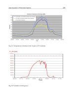
New and more sophisticated measuring techniques for laboratory experiments have been
developed in the last years using advanced optical technology as Laser Induced
Fluorescence (LIF) and Particle Image Velocimeter (PIV). With these techniques the
concentration and velocity fields can be completely characterized. Results can also be used
to calibrate and validate complex CFD (Computational Fluid Dynamics) numerical models.
Table 3 shows the experimental coefficient values obtained by experimental research,
focused on negatively buoyant jet discharges into stagnant environment:

NEGATIVELY BOUYANT SINGLE JET IN STAGNANT ENVIRONMENT.
RESEARCH
α

Nº
Froude
t
y
D

i
x
D

i
S
30º 25-60 1.04F 3.48 -
45º 25-60 1.56F 3.33 -
Zeitoun et al (1970)
Conventional techniques

60º 25-60 2.13F 3.19 1.12F
Roberts et al, (1997)
Optical techniques
60º 18-36 2.2F 2.4F 1.6F+/-12%
30º 18-32 1.08 3.03 -
45º 18-32 1.61 2.82 -
Cipollina et al (2009)
Convencional techniques
60º 18-32 2.32 2.25 -
30º 27-50 1.07 3.18 1.51
45º 27-50 1.71 3.332 1.71
Kikkert et al (2007)
(LA)
Optical techniques
60º 27-50 2.2 2.79 1.81
30º 18-36 1.05 3 1.45
Shao et al (2010)
Optical Techniques
45º 18-36 1.47 2.83 1.26
Table 3. Experimental coefficients for dimensional analysis formulas for single port
hyperdense jets (
α
: discharge angle).
3.3 Numerical modelling.
Water quality modelling is a mathematical representation of the physical and chemical
mechanisms determining the development of pollutant concentrations discharged into the
seawater receiving body. It involves the prediction of water pollution using mathematical
simulation techniques and determines the position and momentum of pollutants in a water
body taking into account ambient conditions.
Water quality modelling applied to brine discharges solves the hydrodynamics and

transport equations adapted to a negatively buoyant effluent. The equations can be set up
by a Lagrangian or Eulerian system. In the first case, the effluent brine is represented by a
collection of particles moving in time and changing their properties. In the second case, the
space is represented by a mesh of fixed points defined by their spatial coordinates, on which
differential equations are solved.
Figure 6 shows the modelling scheme for designing brine discharges (Palomar et al, 2010).
Desalination, Trends and Technologies

290

Fig. 6. Scheme of brine discharge modelling.
3.3.1 Symplifying assumptions within modelling.
Simplifying assumptions which are generally taken in the modelling of brine discharges are
(Doneker & Jirka, 2001):
1.
Incompressible fluid (pressure does not affect density of the fluid).
2.
Reynolds decomposition: () () ()
f
tftft
′
=+ the instantaneous value of a magnitude is
the sum of a time-averaged component and a random (instant, turbulent) component.
3.
Boussinesq approximation: density differences between effluent discharges and the
water receiving environment are small and are important only in terms of the buoyancy
force.
4.
Turbulence closure model based on Boussinesq turbulent viscosity theory,
_______

´´
i
ij ei
j
dU
uu
dx
ρρμ
−
= . Turbulent terms are proportional to the average value of the
magnitude, with an experimental proportionality coefficient (eddy viscosity). In recent
years, more rigorous and sophisticated closure models, such as the k-ε model, are being
applied.
5.
Molecular diffusion is negligible compared to turbulent diffusion in the effluent.
6.
There are no fluid sources or drain.
3.3.2 Governing equations.
Once the simplifying assumptions have been applied, the partial differential equations to be
solved in brine discharge modelling are:
Equation of Continuity (Mass Conservation)
It is a statement of mass conservation. For a control volume that has a single inlet and a
single outlet, the principle of mass conservation states that, for steady-state flow, the mass
Impacts of Brine Discharge on the Marine Environment. Modelling as a Predictive Tool

291
flow rate into the volume must equal the mass flow rate out of it. It relates velocity and
density of the fluid.
_
0

i
i
u
x
∂
=
∂
Cartesian coordintes:
___
0
uvw
xy z
⎛⎞
∂∂∂
⎜⎟
+
+=
⎜⎟
∂∂ ∂
⎜⎟
⎝⎠

Equation of momentum conservation
The momentum equation is a statement of Newton's Second Law and relates the sum of the
forces acting on a fluid element (incompressible) to its acceleration or momentum change
rate:
_
_
dp
F

dt
∑=
. Total force is the sum of surface forces (viscous stresses) acting by direct
contact, and volume forces (inertial) acting without contact

2
3
1
i
ieii
o
Du
p
gu
Dt
δμ
ρ
→
→→
=− ∇ − + ∇ Cartesian coordinates:
X Axis: →
_ _ _ _ ___
222
__ _
222
oex
p
u u u u uuu
uvw
txy z x

xyz
ρμ
⎛⎞⎛⎞
∂
∂ ∂ ∂ ∂ ∂∂∂
⎜⎟⎜⎟
+++ =−+ ++
⎜⎟⎜⎟
∂∂∂ ∂ ∂
∂∂∂
⎜⎟⎜⎟
⎝⎠⎝⎠

Y Axis →
_ _ _ _ ___
222
__ _
222
oey
p
v v v v vvv
uvw
txy z y
xyz
ρμ
⎛⎞⎛⎞
∂
∂ ∂ ∂ ∂ ∂∂∂
⎜⎟⎜⎟
+++ =−+ ++

⎜⎟⎜⎟
∂∂∂ ∂ ∂
∂∂∂
⎜⎟⎜⎟
⎝⎠⎝⎠

Z Axis →
_ _ _ _ ___
222
___
222
oez
p
w w w w www
uvw g
txy z z
xyz
ρ
μρ
⎛⎞⎛⎞
∂
∂∂∂ ∂ ∂∂∂
⎜⎟⎜⎟
+++ =−+ ++ −
⎜⎟⎜⎟
∂∂∂ ∂ ∂
∂∂∂
⎜⎟⎜⎟
⎝⎠⎝⎠


Transport equation (Conservation of Solute mass)
For a control volume, changes in concentration (salinity) are due to: advective transport of
fluid containing the substance, solute mass flow by diffusion, and destruction or
incorporation of the substance in the fluid.
Cartesian coordinates:
___ _ _ _ _
__ _
xyz
ccc c c c c
uvw
txy zxxyyzz
εεε
⎛⎞⎛⎞⎛⎞
∂
∂∂ ∂∂∂∂∂∂∂
⎜⎟⎜⎟⎜⎟
+++ = + +
⎜⎟⎜⎟⎜⎟
∂
∂∂ ∂∂∂∂∂∂∂
⎜⎟⎜⎟⎜⎟
⎝⎠⎝⎠⎝⎠

Equation of State.
For an incompressible fluid, relates temperature, salinity and density. Normally the
empirical equation of the UNESCO is used. Salinity is expressed in "psu (practical salinity
units) and is calculated through fluid conductivity:
2324364
95 3 52 73 94
34

( , ) 999.842594 6.793952 10 9.09529 10 1.001685 10 1.120083 10
6.536332 10 (0.824493 4.0899 10 7.6438 10 8.2467 10 5.3875 10 )
( 5.72466 10 1.0227 10 1.6546
TS T T T T
TTTTTS
T
ρ
−− − −
− −−−−
−−
=+⋅−⋅+⋅−⋅+
+⋅+ −⋅+⋅−⋅+⋅
+
+− ⋅ + ⋅ − ⋅
62 1.5 42
10 ) 4.8314 10TS S
−−
+⋅

Desalination, Trends and Technologies

292
Variables in the equations are:
p
: Fluid pressure at position (x, y, z).
(,, )uvw : Time averaged velocity components.
ρ
: Effluent density at position (x,y,z).
ei
μ

: Fluid dynamic viscosity of the fluid.
ν
: Eddy viscosity
i
ε
: Turbulent diffusion coefficient.
c : Pollutant concentration, in this case: salinity, at position (x,y,z).
o
U ;
o
V ;
o
Q ;
o
ρ
: velocity, volume, flow and density of the effluent at discharge.
A
U ;
A
V ;
A
Q ;
A
ρ
: velocity, volume, flow and density of the receiving seawater body.
:D diameter of the orifice.
'
oA
o
ref

gg
ρ
ρ
ρ
−
=
: reduced gravitational buoyancy acceleration.
The variables "x" time averaged are expressed through an upper dash.
3.3 Model types according to mathematical approach.
There are three basic approaches for solving the equations according to the hypothesis and
simplifications assumed, resulting in three types of physical and mathematical models to
describe the behaviour of a discharge (Doneker &Jirka, 2001):
-
Models based on a dimensional analysis of the phenomenon.
-
Models based on integration of differential equations along the cross section of flow.
-
Hydrodynamics models.
A) Models based on a dimensional analysis of the phenomenon.
The length scale models, derived from a dimensional analysis of the phenomenon, are the
simplest models because they accept important simplifying assumptions.
Dimensional analysis is used to form reasonable hypotheses about complex physical
situations that can be tested experimentally and to categorize types of physical quantities
and units based on their relations to or dependence on other units, or their dimensions if
any.
In dimensional analysis, variables with a higher influence in the phenomenon are
considered, setting up the value of the ones with less influence, to reduce the independent
variables under consideration. Selected independent variables are related through "flux"
magnitudes, which represent the major forces determining effluent behaviour. For the
discharging phenomenon, the main fluxes are:

-
Kinematic flux of mass:
2
0
4
QDU
π
=
. Dimension
3
/LT
⎡
⎤
⎣
⎦
. Represents effluent flow
discharged into the receiving environment.
-
Kinematic flux of momentum:
M
UQ
=
. Dimension:
42
/LT
⎡
⎤
⎣
⎦
. It represents the energy

transmitted during the discharge of the effluent.
-
Kinematic flux of buoyancy: 'JgQ
=
in dimension
43
/LT
⎡
⎤
⎣
⎦
. Represents the effect of
gravity on the effluent discharge.
Fluxes are combined with each other and with other parameters that influence discharge
behaviour (ambient currents, density stratification, jet vertical angle, etc.) to generate length
Impacts of Brine Discharge on the Marine Environment. Modelling as a Predictive Tool

293
scale magnitudes that characterise effluent behaviour. The value of the length scales
depends, anyhow, on the role of the forces acting on the effluent and varies along the
trajectory of the effluent. The main length scales for a round buoyant jet are (Roberts et al,
1997):
Flux-momentum length scale.
1/2
Q
Q
l
M
=
: a measure of the distance over which the volume

flux of the entrained ambient fluid becomes approximately equal to the initial volume flux.
Momentum-Buoyancy length scale.
3/4
1/2
M
M
l
J
= : a measure of the distance over which the
buoyancy generated momentum is approximately equal to the initial volume flux.
Assuming full turbulent flow (thus neglecting viscous forces), any dependent variable will
be a function of the fluxes: Q, M, J. The dependent variables of interest may be expressed in
terms of length scales, with a proportionality coefficient, which is obtained from laboratory
experiments.
,1 2
,(,,)(,)
tii QM
y
XS
f
QMJ
f
ll
=
=
Considering
QM
ll<< , assuming Boussinesq hypothesis for gravity terms and using the
equivalent expression obtained by substituying the values of
M

and J in the
M
l
expression:
1/4
4
M
lDF
π
⎛⎞
=•
⎜⎟
⎝⎠
, the variables of interest will depend on the diameter orifice
and the Densimetric Froude number:
1
t
y
C
DF
=
;
2
i
X
C
DF
=
;
3

i
S
C
F
=

Being:
t
y : maximum rise height (maximum height of the top boundary or upper edge of the jet).
i
X : horizontal distance of centerline peak at the impact (impingement) point
i
S : minimum centerline dilution at the impact point.
U: discharge velocity.
D: diameter of the orifice.
F: Densimetric Froude number.
123
,.CCC : experimental constants or coefficients obtained from laboratory physical scale
models (for a stagnant environment, different discharge angles, etc.).
As already explained, the dimensional analysis derives from highly simplified formulas for
the characterization of the flow because governing equations are reduced to semi-empirical
expressions of length scales. Since this method does not solve rigorous equations of the
phenomenon, its reliability would depend on the range and quality of the experimental tests
performed.
Some examples of the length scale models for brine discharge modelling are those showed
in section 3.2, with the experimental coefficients obtained by several authors and showed in
Table 3. Dimensional analysis formulas are also those used for CORMIX1 (Doneker & Jirka,
Desalination, Trends and Technologies

294

2000), and CORMIX2 (Akar & Jirka, 1991) subsystems of the CORMIX software (Doneker &
Jirka, 2001).
B) Models based on the integration of differential equations.
Governing equations of flow are in this case integrated over the cross section, transforming
them into simple ordinary differential equations which are easily solved with numerical
methods, as Runge Kutta formula. These integration models are mainly used for jets and
gravity current modelling.
Integration of the equation requires assumption of an unlimited receiving water body and
consequently boundary effects cannot be modelled. Because of this, even if these models
give detailed descriptions of the jet effluent, results are valid only in the effluent trajectory
prior to the impact of the jet on the bottom, and whenever the effluent does not previously
reach the surface or impact with obstacles or lateral boundaries. Since the results of the
integrated equation refer to magnitudes in the brine effluent axis, calculations of these
values in cross-sections require assuming a distribution function, generally Gaussian, and
experimentally determining the basic parameters. Effluent diffusion is controlled in these
models through simple “entrainment” formulas with coefficients obtained experimentally.
Commercial models of this type are: CORJET (Jirka, 2004, 2006) of CORMIX software; JetLag
of VISJET software (Lee & Cheung, 1990) and UM3 of VISUAL PLUMES (Frick, 2004), all of
them available for negatively buoyant discharges.
Some of the advantages of integration models are (Palomar & Losada, 2008): equation
solving and calibration are quite easy and need few input data for modelling. Among the
disadvantages is the unlimited receiving water, which limits brine discharges modelling to
the near field region.
C) Hydrodynamic models
Hydrodynamics three-dimensional models are the most general and rigorous models for
effluent discharge simulation. They solve differential hydrodynamics and transport
equations with complete partial derivates. These models require a great number of initial
data but can consider more processes and variables such as: boundary effects, bathymetry,
salinity/ temperature (density) water columns stratification, ambient currents at different
depths, waves, tides, etc.

Among their advantages are: more rigorous and complex phenomena modelling, possibility
of continuous simulation of the near and far field region, simulation of any discharge
configuration and ambient conditions.
At present, these models are not completely developed and have some limitations such as:
coupling between the near and far field regions, because of the different spatial and time
scales; need of a large amount of initial data; difficulty in calibration of the model and long
computational time.
Hydrodynamics three dimensional models are: COHERENS software (Luyten et al, 1999),
DELFT3D], etc.
3.4 Commercial tools for brine discharge modelling.
Nowadays there are many commercial tools for discharge modelling and some of them are
adapted to simulate negatively buoyant effluents, as that of brine. These tools solve the
numerical equations with approaches such as those explained in the previous section,
considering the most relevant processes and determining the geometry and saline
concentration evolution of the effluent.
Impacts of Brine Discharge on the Marine Environment. Modelling as a Predictive Tool

295
CORMIX, VISUAL PLUMES and VISJET are some of the most notable commercial software
for brine discharge modelling. The models predict brine behaviour, including trajectory,
dimensions and dilution degrees, considering the effluent properties (e.g., flow rate,
temperature, salinity, etc.), the disposal configuration and the ambient conditions (e.g., local
water depth, stratification, currents, etc.). Commercial models are often used by promoters to
design the discharge and by environmental authorities to predict potential marine impacts.
Figure 7 shows images and schemes of numerical results obtained by commercial software:


CORMIX, VISUAL PLUMES and VISJET include several models to simulate brine
discharges through different types of discharge configuration. Table 4 shows the software
models adapted to negatively buoyant effluents modelling:


CORMIX software
VISUAL PLUMES
software
VISJET software
CORMIX 1: submerged and emerged
single port jet.
CORMIX 2: submerged multiport jets
D-CORMIX: Direct surface discharge
CORJET: submerged single and
multi-port jets
UM3: submerged jets
single and multi-port

JetLag; submerged jets
single and multi-port

OTHER MODELS OF THE COMMERCIAL SOFTWARE
CORMIX3: for positively buoyant
effluents
DKHW, RSB: only positively buoyant effluents
Table 4. Software models for brine discharge modelling.
3.4.1 CORMIX software.
CORMIX software (Cornell Mixing Zone Expert System) (Doneker & Jirka, 2001) was
developed in the 1980s at Cornell University as a project subsidized by the Environmental
Protection Agency (EPA). Since it was supported by EPA, it has become one of the most
popular programs for discharge modelling.
CORMIX is defined as a Hydrodynamic Mixing Zone Model and Decision Support System
for the analysis, prediction, and design of aqueous toxic or conventional pollutant
discharges into diverse water bodies. It is an expert system, which also includes various

subsystems for simulating the discharge phenomenon.
The subsystems: CORMIX 1, 2 and 3 are based on dimensional analyses of the phenomenon
while the model CORJET is based on the integration of differential equations. CORMIX can
simulate disposals of effluents with positive, negative and neutral buoyancy, under different
types of discharge (single port and multiple port diffusers, emerged and submerged jets,
Desalination, Trends and Technologies

296
surface discharges, etc.) and ambient conditions (temperature/salinity, currents direction
and intensity, etc.).
CORMIX is a steady state model, therefore time series data and statistical analyses cannot be
considered.
CORMIX1: SUBMERGED SINGLE PORT DISCHARGES.
CORMIX1 (Doneker & Jirka, 1990) is the CORMIX subsystem applicable to single port
discharges. Regarding negatively buoyant effluents, CORMIX1 can simulate submerged and
emerged jets.
The model is based on a dimensional analysis of the phenomenon. The subsystem calculates
flows, length scales and dimensionless relationships, and identifies and classifies the flow of
study in one of the 35 flux classes included in its database. Once the flow has been classified,
simplified semi-empirical formulas are applied in order to calculate the main features of the
brine effluent behaviour.
CORMIX1 can make a roughly approximation of the brine effluent’s behaviour in the near
and the far field regions. CORMIX1 simulates the interaction of the flow with the contours
and if no interaction is detected, it applies the model CORJET. CORMIX1 includes some
terms to consider the COANDA attachment effect.
The main assumptions of CORMIX1 are:
-
Since calculation formulas are mainly empirical, reliability depends on the quality and
approach of the case study to the experiments used to calibrate the formulas.
-

Unrealistically sharp transitions in the development of flow behaviour, for example:
from the near to the far field region.
-
"Black box" formula based on volume control for the characterization of some flux
regions.
-
Water body geometry restrictions: rectangular, horizontal and flat channel receiving
water bodies. Limitations related to the port elevation with respect to the position of the
pycnocline in a stratified water column.
-
Unidirectional and steady ambient currents
-
If flow impacts the surface, depending on water depth, CORMIX1 makes the
simplification of flow homogenized in the water column, etc.
The initial data for CORMIX1 are: temperature, salinity or density of the effluent, pollutant
concentration, jet discharge velocity or brine flow, diameter of the orifice, discharge angle,
local water depth, port elevation, ambient salinity and temperature or ambient density,
ambient current velocity and direction, among others.
One of the main limitations of CORMIX1 is the lack of validation studies for negatively
buoyant effluents. Studies presented in the CORMIX1 manual only include the case of a
vertical submerged jet discharged in a dynamic receiving water body, and the validation is
restricted to trajectories, but not dilution rates. Other shortcoming is that in many cases the
flux classification assumed by CORMIX1 does not match with the type of flow observed in
the laboratory experiments. It is also important to be careful when using CORMIX1 since it
is very sensitive to changes of input data and occasionally small changes in the data values
lead to a misclassification of the flow in another flux class, resulting a completely different
behaviour.
Some recommendations for using CORMIX1 in brine discharge modelling are: if a single jet
with no interaction with the contours is to be designed, it is recommended to utilize the
CORJET module instead of CORMIX1, or utilize both and compare the results to ensure that

Impacts of Brine Discharge on the Marine Environment. Modelling as a Predictive Tool

297
the classification of the flow is correct and the results are consistent. Given the strong
simplifying assumptions imposed and the lack of validation data, CORMIX1 should be
avoided for simulations of single port brine discharges impacting the surface.
CORMIX 2: SUBMERGED MULTI-PORT DISCHARGES
CORMIX2 (Akar & JIrka, 1991) is the CORMIX subsystem applicable to submerged
multiport discharges.
The model is based on a dimensional analysis of the phenomenon. The subsystem calculates
flows, length scales and dimensionless relationships, and identifies and classifies the flow of
study in one of the 31 flux classes included in its database. Once, the flow has been
classified, simplified semi-empirical formulas are applied to characterize brine behaviour.
CORMIX2 can make a rough approximation of the brine effluent behaviour in the near and
far field regions. CORMIX2 simulates the interaction of the flow with the contours and if no
interaction is detected, it applies the model CORJET. CORMIX1 includes some terms to
consider the COANDA attachment effect. One of the most important advantages of
CORMIX2 is the possibility of modelling merging phenomena when contiguous jets interact.
The main assumptions of CORMIX2 are:
-
If CORMIX2 detects merging between contiguous jets, it assumes the hypothesis of a
equivalent slot diffuser, in which the discharge from the diffuser of equally spaced
ports is assumed to be the same as a line slot discharge with the same length, brine flow
rate and momentum as the set of ports. This assumption makes the model to consider a
two-dimensional flow, with a uniform distribution across the section.
-
As CORMIX1: since the calculation formulas are mainly empirical, reliability depends
on the quality and the approach of the case studies of the experiments used to calibrate
the formulas. Unrealistically sharp transitions in the evolution of flow behaviour and
simplified receiving water body and "Black box" formulas are applied.

-
Although CORMIX2 supposedly simulates a large variety of diffuser multi-port
configurations (unidirectional, staged, alternating diffusers; same direction and fanned
out jets), important assumptions are made, all cases leading to two types: a
unidirectional diffuser with perpendicular jets and a diffuser with vertical jets. This fact
causes important errors in the case of negatively buoyant effluents.
CORMIX2 initial data are: temperature, salinity or density of effluent, pollutant
concentration, jet discharge velocity or brine flow, discharge angle, diameter of the orifices,
port elevation, diffuser length, port spacing, number of ports, local water depth, ambient
salinity and temperature and current velocity and direction, among others. An important
shortcoming of CORMIX2 is the assumption applied to bilateral or rosette discharges, in
which CORMIX2 considers the jets merging in a unique vertical single jet. This assumption
is roughly correct for positively buoyant effluents whereas it is not valid for negatively
buoyant effluents, leading to completely wrong results. The equivalent slot diffuser
hypothesis leads in some cases to unrealistic results.
The limitations are similar to those of CORMIX1 in relation to receiving water body
geometry simplifications, lack of validation studies for hyperdense effluents, or sensitivity
to initial data variations.
Some recommendations for using CORMIX2 in brine discharge modelling are: given the
strong simplifying assumptions imposed and the lack of validation data, CORMIX2
subsystem should be avoided in the case of flux interacting with contours. Due to the
invalid hypotheses assumed, CORMIX2 cannot be used with bidirectional and alternating
Desalination, Trends and Technologies

298
diffusers, rosettes and unidirectional diffuser with jets forming less than 60º. The typical
diffuser configuration with bidirectional jets forming 180º should be modelled by CORMIX2
considering separately each diffuser side.
CORJET: CORNELL BUOYANT JET INTEGRAL MODEL
CORJET is a model of CORMIX applicable to submerged single port (Jirka, 2004) and multi

port discharges (Jirka, 2006).
It is a three dimensional eulerian model based on the integration of the differential
equations of motion and transport through the cross section, obtaining the evolution of the
jet axis variables. The integration of the differential equations transforms them into an
ordinary equation system, which is solved with a four order Runge Kutta numerical
method. Integration requires assuming an unlimited receiving water body and sections self
similarity. Regarding the variables distribution in the jet cross section, CORJET assumes
Gaussian profiles since it has been experimentally observed in round jets.
Since the model assumes unlimited environment, it cannot simulate the interaction of the jet
with the contours, thus the scope is limited to the near field zone, before the impingement of
the jet with the bottom. The COANDA effect and intrusion are not modelled by CORJET. As
CORMIX1 and CORMIX2, CORJET validation studies are very scarce and limited to the jet
path with few dilution data (Jirka, 2008). Regarding the diffuser configuration, CORJET can
only model unidirectional jets perpendicular to the diffuser direction, with the same
diameter orifices, equal spaces, and with the same port elevation and discharge angle.
CORJET initial data are similar to those indicated for CORMIX1 and CORMIX2, with the
advantage of a more detailed description of the flux, with the evolution of the variables of
interest (axis trajectory (x,y,z), velocity, concentration, etc.)
For calculating the jet upper edge position it is recommended to add to the maximum height
axis (zmax), the radius, calculated with the formulas
2rb= or 2rb
=
, “b” being the radial
distance in which the concentration is 50% and velocity amounts to 37% of axis
concentration and velocity respectively. The
2rb= value stands for the radial distance in
which the concentration is 25% and velocity is 14% of that in the jet axis. The value
2rb=
stands for the radial distance in which the concentration is 6% and velocity is 2% of that in
the jet axis. The user must verify that the jet does not impact the surface by calculating this

addition.
Since CORJET cannot simulate COANDA effects it is recommended not to simulate jets with
a discharge angle smaller than 30º and zero port height. Since it does not either model
reintrusion phenomena, discharge angles larger than 70º should not be simulated with
CORJET.
3.4.2 VISUAL PLUMES software.
VISUAL PLUMES (Frick, 2004) is a software developed by the Environment Protection
Agency (EPA), which includes several models to simulate positively, negatively and
neutrally buoyant effluents discharged into water receiving bodies.
VISUAL PLUMES considers the effluent properties, the discharge configuration and the
ambient conditions (temperature, salinity and currents whose intensity and direction can be
variable through the water column). It is limited to the near field region modelling and does
not simulate the interaction of the flow with the contours. VISUAL PLUMES can consider
time series data, simulating discharges under scenarios which change over time.
Impacts of Brine Discharge on the Marine Environment. Modelling as a Predictive Tool

299
“UM3” MODEL (UPDATED MERGE 3D): SINGLE AND MULTI-PORT DIFFUSER.
UM3 is the only model of VISUAL PLUMES applicable to negatively buoyant effluents. It is
a three dimensional lagrangian model which simulates the behaviour of submerged single
or multi port jet discharges into stagnant or dynamic environments. It is based on the
integration of motion and transport differential equations, and shows the evolution of the
variables along the jet axis. As CORJET, UM3 also assumes an unlimited receiving water
body and sections self similarity, but it considers a uniform (“top hat”) distribution of the
variables across the section.
UM3 includes the possibility of simulating a tide effect on the behaviour of the discharge.
The water column can be separated into layers with different temperature and salinity
values, and velocity or intensity of currents.
As a model based on the integration of differential equations, it cannot simulate COANDA
effects, reintrusion phenomena or interaction of the flow with the contours, so its scope is

limited to the point before jets impinge with the bottom. Regarding the diffuser
configuration, UM3 can only model unidirectional jets perpendicular to the diffuser’s
direction, with the same diameter orifices, equal spaces, and with the same port elevation
and discharge angle.
No validation data have been found in the literature for negatively buoyant effluents
modelled with UM3.
Some recommendations are: the user must enter at least two levels (surface and depth) to
run the model; UM3 does not break when the jet impacts the bottom so the user must be
careful to reject results beyond this point. UM3 considers a uniform distribution of
magnitudes in the cross section, thus if UM3 dilutions are compared with CORJET axis
dilutions, the following formula must be applied: /1.7
axis Top Hat
DD
−
=
.
3.4.3 VISJET Software.
VISJET software (Innovative Modeling and Visualization Technology for Environmental
Impact Assessment) has been developed by the University of Hong Kong.
JETLAG MODEL (LAGRANGIAN JET MODEL): SINGLE AND MULTI-PORT
DIFFUSERS.
JetLag is a three dimensional lagrangian model which simulates single and multi-port
submerged jet discharges. It can simulate positively, negatively and neutrally buoyant
effluents, considering stagnant or dynamic water environments.
JetLag does not strictly resolve the mathematical governing equations, but makes an
approximation of the physical processes, considering entrainment phenomena, in each slice
in which the jet has been previously discretized. It assumes section self similarity and
considers a uniform (“Top Hat”) distribution of the variables in the cross section.
Among its possibilities, it can consider tidal effects on the effluent behaviour. Water column
can be discretized into layers, with different temperature or salinity values, and ambient

currents. JetLag allows different designs for each jet, i.e.: a different diameter in each orifice,
different port elevations, angles of discharge, velocity, etc., in each jet. This fact is due to the
fact that JetLag calculates each jet independently.
JetLag cannot simulate the COANDA effect, the intrusion phenomenon or the interaction of
the flow with the contours. Because of this, JetLag is limited to the point before the jet
impacts the bottom. An important shortcoming of Jetlag, which the users should take into
Desalination, Trends and Technologies

300
account, is that the model does not consider the merging between jets although it seems to
do that. Thus, the choice of diffuser type is not relevant since JetLag always calculates each
jet individually as a single port. JetLag cannot consider time series.
Some recommendations for using JETLAG in brine discharge modelling are: the user must
enter at least two vertical levels in the discretization of the vertical column. Because Jetlag
only simulates single individual jets and cannot calculate merging between jets, it should
not be used for multi-port diffuser modelling. The user must calculate the upper edge of the
jet and calculate if it impacts the surface (invalidating the model) since JetLag only fails
when the axis impacts the surface. JetLag results can be directly compared with UM3 since
both assume a uniform distribution.
3.5 Research related to brine discharge behaviour and modelling: State of art.
The first research related to brine discharge behaviour started in the 1940s in the United
States, and increased radically during the 1960 and 1970 decades.
Regarding the description of the near field region, Turner, 1996, carried out a dimensional
analysis of the phenomenon and established length scales for jet characterization,
considering those variables with strongest influence. Some years later, Turner conducted
physical (scale) laboratory tests to determine experimental coefficient values for the
maximum rise height of a negatively buoyant vertical jet in stagnant waters. Other authors,
such as Holly et al, 1972, followed this line, but extended the studies to other geometrical jet
characteristics. Zeitoun et al, 1970, studied the influence of the discharge angle on jet
behaviour for 30º, 45º, 60º and 90º angles, obtaining the highest dilution with 60º angles.

Since then 60º has been established as the optimum angle for hyperdense jet discharges.
Gaussian profiles along jet cross sections were also observed by Zeitoun. Pincince & List,
1973, based on Zeitoun´s results, studied the effect of dynamic environments in a 60º jet,
concluding that they increase dilution. Chu, 1975, proposed a theoretical model. Fisher et al,
1979, described the three fluxes which are the base of dimensional analysis in relation to
round buoyant jets. Roberts & Toms, 1987, studied the behaviour of vertical and 60º jets into
stagnant and dynamic receiving environments. A significant quantity of laboratory tests
were carried out obtaining experimental coefficients for dimensional analysis formulas.
Roberts et al, 1997, developed new experiments using optical Laser Fluorescence induced
(LIF) techniques for a more rigorous study of a 60º hyperdense jet, discharged on a stagnant
environment.
Cipollina et al, 2005, developed a numerical model for hyperdense jets discharged into a
stagnant environment, based on the integration of differential equations. Jirka, 2004,
proposed a more complex eulerian three dimensional integration model for stagnant and
dynamic environments. This same author (Jirka, 2006) extended his model to multiport
discharges, considering the interaction or merging of jets. Jirka, 2008, introduced the effect
of the bottom slope on jet behaviour. Cipollina et al, 2009, presented new experimental
coefficients for dimensional analysis formulas.
During the last decade, several authors have performed experimental research using
advanced optical techniques, as LIF and PIV, in order to acquire a better knowledge of jet
velocity and concentration fields. Ferrari, 2008, studied 60º and 90º jets in stagnant and wavy
environments. Chen et al, 2008, also considered the effect of waves on jets.
Kikkert & Davidson, 2007, proposed an analytical model for single jet modelling and
calibrated it with experimental coefficients obtained from physical scale tests, using LIF and
Impacts of Brine Discharge on the Marine Environment. Modelling as a Predictive Tool

301
LA techniques. Kikkert compared his results with those of other authors. Papanicolaou et al,
2008, reviewed the entrainment state of the art and proposed new values for negatively
buoyant effluents. Gungor & Roberts, 2009, studied the behaviour of a vertical jet in a

dynamic environment. Recently, Shao, 2010, carried out physical scale experiments with 30º
and 60º jets, taking measurements with PIV and LIF optical techniques, and obtained
experimental coefficients for dimensional analysis formulas. Plum, 2008, applied the
commercial CFD software FLUENT for brine modelling, analysing different turbulence
models.
Regarding the far field region, where brine forms a gravity current, the first important
research was carried out by Ellison & Turner, 1959, who developed a two dimensional
integration model with a simple entrainment formula. The authors experimentally proved
that, at some distance from the discharge point, the plume takes a Richardson number
constant value. Fietz & Wood, 1967, considered a three dimensional plume and analyzed the
influence of the discharge. Alavian, 1986, proposed a three-dimensional integration model
and distinguished between supercritical and subcritical behaviours. Garcia, 1996, presented
an interesting two dimensional integration model based on the eddy viscosity formula for
entrainment. Raithby et al, 1988, applied a more complex turbulence model in a three-
dimensional hydrodynamic model, calibrating it with experimental results.
Regarding entrainment phenomena research, Turner, 1986, studied the mixing associated to
turbulence movement and the effect of viscosity in effluent mixing and behaviour. Kaminski
et al, 2005, experimentally and theoretically studied turbulent entrainment in jets with
arbitrary buoyancy. Papanicolau et al, 2008, studied the entrainment phenomenon in
negatively buoyant jets.
Alavian at al, 1992, expanded their study to a three-dimensional flow moving in a stratified
environment. Tsihrintzis & Alavian, 1986, experimentally obtained an equation for
calculating the plume width in a laminar regime. Christodoulou & Tzachou, 1979, simulated
the behaviour of three-dimensional gravity currents in scaled tanks and obtained formulas
for calculating the velocity, the width and the thickness of the gravity current. Cheong &
Han, 1997, studied the influence of the bottom slope in plume behaviour. Bournet et al,
1999, applied different turbulence closure models, performing laboratory experiments and
obtaining coefficients for dimensional analysis formulas.
Ross et al, 2001, presented a model based on integration equations to simulate a gravity
current on a sloping bottom, and supported it with laboratory data, including geometry and

dilution. Özgökmen & Chassignet, 2002, studied the behaviour of a plume, varying the
parameters of interest and considering small-scale turbulence.
Bombardelli et al., 2004, studied three-dimensional gravity currents using CFDs
(Computational Fluid Mechanics) models, capturing small-scale turbulent phenomena, and
comparing the results obtained using different commercial software. Oliver et al, 2008,
discussed the mixing of a hypersaline plume with ambient fluid using a closure model for
turbulent terms. Joongcheol Paik et al, 2009, used a three dimensional RANS equations
model to simulate a two-dimensional plume, comparing experimental data with numerical
results using different turbulence closure models.
Dallimore et al, 2003. used an underflow model coupled to a three dimensional
hydrodynamic model, comparing numerical results with field data. Martin & García, 2008,
conducted an experimental research combining optical PIV/LIF measurements to study
gravity currents. Recently, Hodges et al, 2010, modelled a real case of a brine discharge
gravity current from a desalination plant in Texas (U.S).
Desalination, Trends and Technologies

302
3.6 Shortcomings and research line proposal.
The following paragraphs illustrate the main shortcomings detected in the different fields
related with brine discharge modelling and the knowledge of impact on the marine
environment, proposing some research lines.
As regards the
effects on the marine environment, it is necessary to establish critical
salinity limits, in statistical terms, for ecologically important species which are sensitive to
hyper-salinity and are located in areas of frequent brine discharges. It is also important to
carry out additional studies regarding the synergistic effects of different effluent discharges,
as is the case of brine mixed with cooling water or seawater waste effluents.
Regarding
regulations, a new legislation regulating brine discharges, which includes
emission limit values and quality standards in the environment is still necessary. Regulation

defining dimensions of the mixing zone would be also interesting.
Regarding
brine discharge systems, some discharge configurations such as direct surface
disposal, discharge on gravel beaches, on the mouth of channels flowing to seawaters,
discharge on a breakwater sheltered dock or overflow spillway in a cliff discharge, among
others, are in need of further investigations. Research must be focused on quantitative
descriptions, including dilution rates and modelling.
As regards
methodologies, new ones are needed for brine discharge systems design and
marine impact assessment, that describe all the aspects that need to be taken into account.
Regarding
brine discharge modelling, the following research is proposed to improve
current knowledge on the matter (Palomar & Losada, 2010):
-
Methodology to describe the marine climate and selection of the ambient scenarios in
statistical terms, including the most frequent and unfavourable conditions.
-
Further investigation of the entrainment phenomenon for negatively buoyant effluents.
-
Recalibration of numerical models with experimental coefficients obtained from
experimental measurements carried out with the most rigorous and precise optical
techniques developed in the last years.
-
To improve the knowledge of the gravity currents behaviour and to develop tools for
three dimensional numerical modelling, considering the effect of bathymetry, waves,
bottom currents, environment stratification, etc.
-
To study the possibility of coupling near and far field processes modelling.
To improve the knowledge in some of these areas, several investigation projects are being
developed. One of the most important in the Mediterranean area is the project “Horizon

2020 initiative” which aims to eliminate pollution in the Mediterranean by the year 2020 by
tackling the sources of pollution, including brine from desalination plants. In Spain, the
following projects, financed by the Ministry of Environment, are being developed to
improve brine discharge knowledge and methodologies:
-
ASDECO project (Automated control system for Desalination dilution), the objectives
of which are: to design, develop and validate a prototype of the Automatic Control of
Toxic Desalination; analyzing real-time ocean-meteorological data of the receiving
environment and effluent data (all recorded by the system itself ASDECO), focusing on
its application in brine discharge environmental monitoring plans.
-
VENTURI project (Portillo, 2010), , which aims to test the efficiency in the dilution
degree of Venturi systems as compared to conventional broadcasters, for single port
submerged jet discharges, while “ad hoc” studying the near and far field regions of a
brine discharge in the Canary Islands (Atlantic Ocean).
Impacts of Brine Discharge on the Marine Environment. Modelling as a Predictive Tool

303
- MEDVSA project (Palomar et al, 2010) which aims to develop a methodology in order
to improve brine discharge system design to reduce the impacts of brine discharges on
the marine environment. The objective is to make compatible the use of desalination as
an important water resource in some Spanish coastal areas, with the protection of
marine areas, while following Sustainable Development principles. Two important
Spanish Research Centres: IH Cantabria and CEDEX are collaborating in the R&D
project “MEDVSA” development. It includes the following tasks: experimental research
(Scale physical models), numerical research for near and far field simulations (including
commercial tool analysis, online MEDVSA tools, using CFDs for near field modelling
and ROMS application for far field simulation, etc.); climate scenario research;
numerical tool validation (field works and experimental tests); a methodological guide
and dissemination and training. Regarding commercial tools analysis, CORMIX,

VISUAL PLUMES and VISJET, focused on negatively buoyant effluents, have been
analyzed in detail. As a result, Technical Specification Cards have been developed,
including: theoretical basis, simplifying assumptions, modelling options, possibilities
and limitations and recommendations for implementation and management. After
having analyzed in detail the brine discharge commercial simulation tools and having
reviewed the existing literature on the matter, different codes are being programmed in
order to have freely accessible tools, with codes similar to those of the commercial
software. These tools will be calibrated and validated with the results of new laboratory
tests. Technical Specification Cards and MEDVSA online tools are available and can be
downloaded from the Web Page of the MEDVSA project.
4. Recommendations on the design and modelling of brine discharges into
the sea.
In order to improve design of brine discharge systems, the following paragraphs propose
some recommendation for reducing marine environment impacts faced to these disposals
(Palomar & Losada, 2010):
-
Brine disposal should be placed in non-protected areas or in areas under anthropic
influence.
-
The brine discharge system should be placed in areas of high turbulence, where
ambient currents and waves facilitate brine dilution into the receiving water body.
Ambient conditions, including slope, water column stratification and bottom currents
are essential in far field dilution. If the discharge zone is deeper than the area to be
protected, the latter should not be affected, since brine flows down slope to the bottom.
-
The brine discharge configuration should consider the particular characteristics of the
discharge area and the degree of dilution necessary to guarantee compliance with
environmental quality standards and the protection of marine ecosystems located in the
area affected by the discharge.
-

If there are any protected ecosystems along the seabed in the area surrounding the
discharge zone, it is recommended to avoid direct surface brine discharge systems
because the degree of dilution and mixing is very weak.
-
To maximize brine dilution, jet discharge configurations, through outfall structures, are
recommended to be installed. It can be a solution when there are ecologically important
stenohaline species near the discharge area. The following requirements are
recommended to optimize jet discharges:
Desalination, Trends and Technologies

304
• The densimetric Froude number at the discharge must always be higher than 1,
even so the installation of valves is recommended.
• Jet discharge velocity should be maximized to increase mixing and dilution with
seawater in the near field region. The optimum ratio between the diameter of the
port and brine flow rate per port is set so that the effluent velocity at discharge is
about 4 – 5 m/s.
• Nozzle diameters are recommended to be bigger than 20cm, to prevent their
clogging due to biofouling.
• To maximize mixing and dilution with submerged outfall discharges, a jet
discharge angle between 45º and 60º with respect to the seabed is advisable, under
stagnant or co-flowing ambient conditions. In case of cross-flow, vertical jets (90º)
reach higher dilution rates (Roberts et el, 1987)- Avoid angles exceeding 75º and
below 30 º.
• Diffusers (ports) should be located at a certain height (elevation) above the seabed,
avoiding the brine jet interaction with the hypersaline spreading layer formed after
the jet impacts the bottom. This port height can be set up between 0.5 and 1.5 m.
• The discharge zone is recommended to be deep enough to avoid the jet from
impacting the surface under any ambient conditions.
• Avoid designs with several jets in a rosette.

• Riser spacing is recommended to be large enough to avoid merging between
contiguous jets along the trajectory, because this interaction will reduce the dilution
obtained in the near field region and also because the modelling tools to simulate
this merging are less feasible.
-
If it is necessary to build a submarine outfall, and it passes through interesting benthic
ecosystems, a microtunnel to locate the pipeline should be constructed.
-
As a prevention measure, modelling tools should be used for modelling discharge and
brine behaviour into seawaters, under different ambient scenarios.
-
An interesting alternative is to discharge brine into closed areas with a low water
renovation rate, or areas receiving wastewater disposals. This mixture is favourable
since it reduces chemicals concentration and anoxia in receiving waters.
-
An environmental monitoring plan must be established, including the following
controls: feedwater and brine flow variables, surroundings of the discharge zone,
receiving seawater bodies and marine ecosystems under protection located in the area
affected by the brine discharge.
Regarding
brine discharge modelling (Palomar & Losada, 2010):
-
Modelling data must be reliable and representative of the real brine and ambient
conditions. Their collection should be carried out by direct measurements in the field.
The most important data in the near field region are: 1) brine effluent properties: flow
rate, temperature and salinity, or density, and 2) discharge system parameters. In the
far field region, mixing is dominated by ambient conditions: bathymetry, density
stratification in the water column, ambient currents on the bottom, etc.
-
In the case of using CORMIX1 or CORMIX2 for brine discharge modelling, it must be

taken into account that both are based on dimensional analysis and thus reliability
depends on the quality of the laboratory experiments on which they are based, and on
the degree of assimilation to the real case to be modelled. The scarcity of validation
studies for negatively buoyant effluents in CORMIX1 and CORMIX2, is one of the main
shortcomings of these commercial tools.
Impacts of Brine Discharge on the Marine Environment. Modelling as a Predictive Tool

305
- For each simulation case, it is recommended to use different models and to compare the
results to ensure that jet dimensions and dilution are being correctly modelled. It is also
recommended to run the case under different scenarios, always within the range of
realistic values of the ambient parameters.
-
With respect to brine surface discharges, most of the commercial codes: RSB and PSD of
VISUAL PLUMES or CORMIX 3 of CORMIX focus on positively buoyant discharges. D-
CORMIX is designed for hyperdense effluent surface discharges but has not yet been
sufficiently validated and therefore cannot be considered feasible at the moment.
-
For far field region behaviour modelling, hydrodynamics three-dimensional or quasi-
three dimensional models are recommended. At present, these models have errors
linked to numerical solutions of differential equations, especially in the boundaries of
large gradient areas, such as the pycnocline between brine and seawater in the far field
region. These errors can be partially solved if enough small cells are used in the areas
where large gradients may arise, but it significantly increases the modelling
computation time.
-
It is necessary to generate hindcast databases of ambient conditions in the coastal
waters which are the receiving big volumes of brine discharges, considering those
variables with a higher influence in brine behaviour. Analysis of this database by means
of statistical and classification tools will allow establishing scenarios to be used in the

assessment of brine discharge impact.
5. Conclusion
Desalination projects cause negative effects on the environment. Some of the most
significant impacts are those associated with the construction of marine structures, energy
consumption, seawater intake and brine disposal.
This chapter focuses on brine disposal impacts, describing the most important aspects related
to brine behaviour and environmental assessment, especially from seawater desalination
plants (SWRO). Brine is, in these cases, a hypersaline effluent which is denser than the
seawater receiving body, and thus behaves as a negatively buoyant effluent, sinking to the
bottom and affecting water quality and stenohaline benthic marine ecosystems.
The present chapter describes the main aspects related to brine disposal behaviour into the
seawater, discharge configuration devices and experimental and numerical modelling. Since
numerical modelling is currently and is expected to be in the future, a very important
predictive tool for brine behaviour and marine impact studies, it is described in detail,
including: simplifying assumptions, governing equations and model types according to
mathematical approaches. The most used commercial software for brine discharge
modelling: CORMIX, VISUAL PLUMES y VISJET are also analyzed including all modules
applicable to hyperdense effluent disposal. New modelling tools, as MEDVSA online
models, are also introduced.
The chapter reviews the state of the art related to negatively buoyant effluents, outlining the
main research being carried out for both the near and far field regions. To overcome the
shortcomings detected in the analysis, some research lines are proposed, related to important
aspects such as: marine environment effects, regulation, disposal systems, numerical
modelling, etc. Finally, some recommendations are proposed in order to improve the design of
brine discharge systems in order to reduce impacts on the marine environment. These
recommendations may be useful to promoters and environmental authorities.
Desalination, Trends and Technologies

306
6. References

Afgan, N.H; Al Gobaisi, D; Carvalho, M.G. & Cumo, M. (1998). Sustainable energy
management.
Renewable and Sustainable Energy Review, vol 2, pp. 235–286.
Akar, P.J. & Jirka, G.H. (1991). CORMIX2: An Expert System for Hydrodynamic Mixing
Zone Analysis of Conventional and Toxic Submerged Multiport Diffuser
Discharges,
U.S. Environmental Protection Agency (EPA), Office of Research and
Development
Alavian, V. (1986). Behaviour of density current on an incline. Journal of Hydraulic
Engineering, vol 112
, No 1.
Alavian, V; Jirka, G.H; Denton, R.A; Jhonson, M.C; Stefan, G.C (1992). Density currents
Entering lakes and reservoirs
. Journal of Hydraulic Engineering, vol 118, No 11.
ASDECO project: Automated System for desalination dilution control:

Bombardelli, F.A; Cantero, M.I; Buscaglia, G.C & García, M.H. (2004). Comparative study of
convergence of CFD commercial codes when simulating dense underflows.
Mecánica
computacional. Vol 23, pp.1187 -1199.
Bournet, P.E; Dartus, D; Tassin.B & VinÇon-Leite.B. (1999). Numerical investigation of
plunging density current
. Journal of Hydraulic Engineering. Vol. 125, No. 6, pp. 584-
594.
CEDEX: Spanish Center of Studies and Experimentation of Publish Works www.cedex.es
Chen, Y.P; Lia, C.W & Zhang, C.K. (2008). Numerical modelling o a Round Jet discharged
into random waves.
Ocean Engineering, vol. 35, pp.77-89.
Christodoulou, G.C & Tzachou, F.E, (1997). Experiments on 3-D Turbulent density currents
.

4th Annual Int. Symp. on Stratified Flows, Grenoble, France.
Chu, V.H. (1975). Turbulent dense plumes in a laminar crossflow. Journal of Hydraulic
research
, pp. 253-279.
Cipollina, A; Brucato, A; Grisafi, F; Nicosia, S. (2005). “Bench-Scale Investigation of Inclined
Dense Jets”.
Journal of Hydraulic Engineering, vol 131, n 11, pp. 1017-1022.
Cipollina, A; Brucato,A & Micale, G. (2009). A mathematical tool for describing the
behaviour of a dense effluent discharge.
Desalination and Water Treatment, vol 2, pp.
295-309.
Dallimore, C.J, Hodges, B.R & Imberger, J. (2003). Coupled an underflow model to a three
dimensional Hydrodinamic models.
Journal of Hydraulic Engineering, vol 129, nº10,
pp. 748-757
Delft Hydraulics Software. Delft Hydraulics part of Deltares. Available from:

Doneker, R.L. & Jirka, G.H. (1990). Expert System for Hydrodynamic Mixing Zone Analysis
of Conventional and Toxic Submerged Single Port Discharges (CORMIX1).
Technical Report EPA 600-3-90-012. U.S. Environmental Protection Agency (EPA).
Doneker, R.L & Jirka, G.H. (2001). CORMIX-GI systems for mixing zone analysis of brine
wastewater disposal. Desalination
(ELSEVIER), vol 139, pp. 263–274.
www.cormix.info/.
Einav, R & Lokiec, F. (2003). Environmental aspects of a desalination plant in Ashkelon.
Desalination (ELSEVIER), vol 156, pp. 79-85.
Impacts of Brine Discharge on the Marine Environment. Modelling as a Predictive Tool

307
Ellison, T.H& Turner, J.S. (1959). Turbulent entraintment in stratified flows. Journal of Fluids

Mechanics, vol 6, part 3
, pp.423-448.
Environmental Hydraulics Institute “IH Cantabria” & Centre of Studies and
Experimentation of Public Works (CEDEX). Project MEDVSA (A methodology for
the design of brine discharges into the seawater),
funded by the National Programme
for Experimental Development of the Spanish Ministry of the
Environment and Rural and
Marine Affairs (2008-2010). Available from:
www.mevsa.es. Technical specification cards
Environmental Hydraulics Institute: IH Cantabria. University of Cantabria, Spain.
www.ihcantabria.com
Fernández Torquemada, Y & Sánchez Lisazo, J.L. (2006). Effects of salinity on growth and
survival of Cymodocea
nodosa (Ucria) Aschernon and Zostera noltii Hornemann”.
Biology Marine Mediterranean, vol 13 (4),
pp 46-47.
Ferrari, S & Querzoli, G. (2004). Sea discharge of brine from desalination plants: a
laboratory model of negatively buoyant jets.
MWWD 2004, 3th International
Conference on Marine Waste Water Disposal and Marine Environment.
Ferrari, S;
Fietz, T.R & Wood, I. (1967). Three-dimensional density currents.
Journal of Hydraulics
Division.
Proceedings of the American Society of Civil Engineers.
Frick, W.E. (2004). Visual Plumes mixing zone modelling software.
Environmental &
Modelling Software (ELSEVIER),
vol 19, pp 645-654.


Gacia, E.; Granata, T.C. & Duarte, C.M. (1999). An approach to measurements of particle
flux and sediment retention within seagrass
Posidonia oceanica meadows. Aquatic
Botany, vol 65,
pp. 255–268.
Gacia, E.; Invers, O.; Ballesteros, E.; Manzanera M. & Romero, J. (2007). The impact of the
brine from a desalination plant on a shallow seagrass
(Posidonia oceanica) meadow.
Estuarine, Coastal and Shelf Science, vol 72, Issue 4, pp.579-590.
García, Marcelo. (1996). Environmental Hydrodynamics. Sante Fe, Argentina: Publications
Center, Universidad Nacional del Litoral.
Gungor, E & Roberts, P.J. (2009). Experimental Studies on Vertical Dense Jets in a Flowing
Current.
Journal of Hydraulic Enginnering, vol 135, No11, pp.935-948.
Hauenstein, W & Dracos, TH. (1984). Investigation of plunging currents lacustres generated
by inflows
. Journal of Hydraulic Research, vol 22, No 3.
Hodges, B.R; Furnans, J.E & Kulis, P.S. (2010). Case study: A thin-layer gravity current with
implications for desalination brine disposal.
Journal of Hydraulic Engineering (in
press).
Hogan, T. (2008). Impingement and Entrainment: Biological Efficacy of Intake Alternatives.
Desalination Intake Solutions Workshop Alden Research Laboratory.
Holly, Forrest M., Jr., & Grace, John L., Jr. (1972). Model Study of Dense Jet in Flowing
Fluid
. Journal of the Hydraulics Division, ASCE, vol. 98, pp. 1921-1933.
Höpner, T & Windelberg, J. (1996). Elements of environmental impact studies on the coastal
desalination plants.
Desalination (ELSEVIER), vol 108, pp. 11-18.

Hópner, T. (1999). A procedure for environmental impact assessment (EIA) for seawater
desalination plants.
Desalination (ELSEVIER), vol 124, pp. 1-12.
Desalination, Trends and Technologies

308
Hyeong-Bin Cheong & Young-Ho Han (1997). Numerical Study of Two-Dimensional
Gravity Currents on a Slope.
Journal of Oceanography, vol. 53, pp. 179 - 192.
Iso, S; Suizu, S & Maejima, A. (1994). The Lethal Effect of Hypertonic Solutions and
Avoidance of Marine Organisms in relation to discharged brine from a
Desalination Plant.
Desalination (ELSEVIER), vol 97, pp. 389-399.
Jirka, G-H. (2004). Integral model for turbulent buoyant jets in unbounded stratified flows.
Part I: The single round jet.
Environmental Fluid Mechanics (ASCE), vol 4, pp.1–56.
Jirka, G. H. (2006). Integral model for turbulent buoyant jets in unbounded stratified flows.
Part II: Plane jet dynamics resulting from multiport diffuser jets.
Environmental
Fluid Mechanics, vol. 6,
pp.43–100.
Jirka, G.H. (2008). Improved Discharge Configurations for Brine Effluents from Desalination
Plants.
Journal of Hydraulic Enginnering, vol 134, nº1, pp 116-120.
Joongcheol Paik, Eghbalzadeh, A; Sotiropoulos, F. (2009). Three-Dimensional Unsteady
RANS Modeling of Discontinous Gravity Currents in rectangular Domains.
Journal
of Hydraulic Engineering, vol 135
, n 6, pp. 505-521.
Kaminski, E; Tait, S & Carzzo, G. (2005). Turbulent entrainment in jets with arbitrary

buoyancy.
Journal of Fluid Mechanics, vol. 526, pp. 361-376.
Kikkert, G.A; Davidson, M.J; Nokes, R.I (2007). “Inclined Negatively Buoyant Discharges”.
Journal of Hydraulic engineering, vol 133, pp.545 – 554.
Lee, J.H.W. & Cheung, V. (1990). Generalized Lagrangian model for buoyant jets in current.
Journal of Environmental Engineering (ASCE), vol 116 (6), pp. 1085-1105.
Luyten P.J., Jones J.E., Proctor R., Tabor A., Tett P. & Wild-Allen K. (1999). COHERENS: A
Coupled Hydrodynamical-Ecological Model for Regional and Shelf Seas: User
Documentation.
MUMM Report, Management Unit of the Mathematical Models of the
North Sea, 914.
www.mumm.ac.be/coherens/.
Martin, J.E; García, M.H. (2008). Combined PIV/LIF measurements of a steady density
current front.
Exp Fluids, 46, pp.265-276
Oliver, C.J; Davidson, M.J & Nokes, R.I. (2008). K-ε Predictions of the initial mixing of
desalination discharges
. Environmental Fluid Mechanics, vol 8: pp.617-625
Özgökmen, T.M. & E.P. Chassignet (2002). Dynamics of two-dimensional turbulent bottom
gravity currents. Journal
of Physical Oceanography, vol 32/5, pp.1460-1478.
Palomar, P & Losada, I.J. (2008). Desalinización de agua marina en España: aspectos a
considerar en el diseño del sistema de vertido para protección del medio marino.
Public civil works Magazine (Revista de Obras Públicas). Nº 3486, pp. 37-52.
Palomar, P & Losada, I.J. (2009). Desalination in Spain: Recent developments and
Recommendations.
Desalination (ELSEVIER), vol 255, pp. 97-106.
Palomar, P; Ruiz-Mateo, A; Losada, IJ; Lara, J L; Lloret, A; Castanedo, S; Álvarez, A;
Méndez, F; Rodrigo, M; Camus, P; Vila, F; Lomónaco, P & Antequera, M. (2010).
“MEDVSA: a methodology for design of brine discharges into seawater” Desalination and

Water Reuse, vol. 20/1,
pp. 21-25.
Palomar, P & Losada, I.J. (2010). “Desalination Impacts on the marine environment”.
Book.
The Marine Environment: ecology, management and conservation”. Edit. NOVA
Publishers.
Submitted.
Impacts of Brine Discharge on the Marine Environment. Modelling as a Predictive Tool

309
Papanicolau, P, Papakonstantis, I.G; & Christodoulou, G.C.(2008). On the entrainment
coefficients in negatively buoyant jets.
Journal of Fluid Mechanics, vol. 614, pp. 447-
470.
Pincice, A.B., & List, E.J. (1973). Disposal of brine into an estuary.
Journal Water Pollution, vol
45 (11),
pp. 2335-2344.
Plum, B.R. (2008). Modelling desalination plant outfalls.
Final Thesis Report. University of New
South Wales at the Australia Defence Force Academy.
Portillo, 2009. Instituto Tecnológico de Canarias. S.A. “Venturi Projects” , funded by the
National Programme for Experimental Development of the Spanish Ministry of the
Environment and Rural and Marine Affairs (2008-2010).
Querzoli, G. (2006) An experimental investigation of interaction between dense sea
discharges and wave motion.
MWWD 2006, 4th International Conference on Marine
Waste Water Disposal and Marine Environment.
Raithby, G.D; Elliott, R.V; Hutchinson, B.R (1988). Prediction of three-dimensional thermal
Discharge flows.

Journal of Hydraulic Division, ASCE 114(7), 720–737
Roberts, P.J.W & Toms, G. (1987). Inclined dense jets in a flowing current.
Journal of
Hydraulic Engineering, vol 113
, nº 3.
Roberts, P.J.; Ferrier, A & Daviero, G. (1997). Mixing in inclined dense jets.
Journal of
Hydraulic Engineering (ASCE), vol. 123, No 8
, pp. 693-699.
Ross, A; Linden, F y Dalziel S.B. (2001). A study os three-dimensional gravity currents on a
uniform slope
. Journal of Fluid Mechanics, vol 453, pp.239-261.
Ruiz Mateo, A. (2007). Los vertidos al mar de las plantas desaladoras” (Brine discharges into
seawaters).
AMBIENTA magazine, vol .51, pp. 51-57.
Sánchez-Lizaso, J.L.; Romero, J.; Ruiz, J.; Gacia, E.; Buceta, J.L.; Invers, O.; Fernández
Torquemada, Y.; Mas, J.; Ruiz-Mateo, A. & Manzanera, M. (2008). Salinity tolerance
of the Mediterranean seagrass
Posidonia oceanica: recommendations to minimize the
impact of brine discharges from desalination plants
. Desalination (ELSEVIER), vol
221
, pp. 602-607.
Shao, D & Wing-Keung Lao. (2010). “Mixing and boundary interactions of 30º and 45º
inclined dense jets”.
Environmental Fluid Mechanics, vol 10, nº5, pp. 521-553.
Terrados, J & Ros, J.D. (1992). Growth and primary production of Cymodocea nodosa (Ucria)
Ascherson in a Mediterranean coastal lagoon: the Mar Menor (SE Spain).
Aquatic
Botany, vol 43

, pp 63-74.
Tsihrintzis, V.A. and Alavian, V. (1986). Mathematical modeling of boundary attached
gravity plumes.
Proceedings Intern. Symposium on Buoyant Flows, G. Noutsopoulos
(ed), Athens, Greece,
pp.289-300.
Turner, J.S. (1966). Jets and plumes with negative or reversing buoyancy.
Journal of Fluid
Mechanics,
vol. 26, pp 779-792.
Turner, J.S (1986). Turbulent entraintment: the development of the entraintment
assumption, and its application to geophysical flows.
Journal of Fluid Mechanics, vol
173,
pp.431-471
VISJET: Innovative Modeling and Visualization Technology for Environmental Impact
Assessment.
Desalination, Trends and Technologies

310
Zeitoun, M.A & McIlhenny, W.F. (1970). Conceptual designs of outfall systems for
desalination plants.
Research and Development Progress Rept. No 550. Office of Saline
Water, U.S. Dept, of Interior.

14
Optimization of Hybrid Desalination Processes
Including Multi Stage Flash and
Reverse Osmosis Systems
Marian G. Marcovecchio

1,2,3
, Sergio F. Mussati
1,4
,
Nicolás J. Scenna
1,4
and Pío A. Aguirre
1,2

1
INGAR/CONICET – Instituto de Desarrollo y Diseño,
Avellaneda 3657 S3002GJC, Santa Fe,
2
UNL – Universidad Nacional del Litoral, Santa Fe,
3
UMOSE/LNEG-Und. de Modelação e Optimização de Sist. Energéticos, Lisboa,
4
UTN/FRRo – Universidad Tecnológica Nacional, Rosario,
1,2,4
Argentina
3
Portugal
1. Introduction
Distillation and reverse osmosis are the two most common processes to obtain fresh water
from seawater or brackish water.
A leading distillation method is the Multi Stage Flash process (MSF). For this method, fresh
water is obtained by applying thermal energy to seawater feed in multiple stages creating a
distillate stream for fresh water uses, and a concentrated (brine) stream that is returned to
the sea.
In Reverse Osmosis processes (RO), the seawater feed is pumped at high pressure to special

membranes, forcing fresh water to flow through the membranes. The concentrate (brine)
remains on the upstream side of the membranes, and generally, this stream is passed
through a mechanical energy recovery device before being discharged back to the sea.
Desalination plants require significant amounts of energy as heat or electricity form and
significant amounts of equipments. Reverse osmosis plants typically require less energy
than thermal distillation plants. However, the membrane replacement and the high-pressure
pumps increase the RO production cost significantly. Furthermore, even the salt
concentration of permeated stream is low; this stream is not free of salt, as the distillate
stream produced by a MSF system.
Therefore, hybrid system combining thermal and membrane processes are being studied as
promising options. Hybrid plants have potential advantages of a low power demand and
improved water quality; meanwhile the recovery factor can be improved resulting in a
lower operative cost as compared to stand alone RO or MSF plants.
Several models have already been described in the literature to find an efficient relationship
between both desalination processes (Helal et al., 2003; Agashichev, 2004; Cardona &
Piacentino, 2004; Marcovecchio et al., 2005). However, these works analyse only specific
fixed configurations for the RO-MSF hybridization.
Desalination, Trends and Technologies

312
In this chapter, all the possible configurations for hybrid RO-MSF plants are analyzed in an
integrated way. A super-structure model for the synthesis and optimization of these
structures is presented. The objective is to determine the optimal plant designs and
operating conditions in order to minimize the cost per m
3
of fresh water satisfying a given
demand. Specifically, the work (Marcovecchio et al., 2009) is properly extended, in order to
study the effect of different seawater concentrations on the process configuration. This will
allow finding optimal relationships between both processes at different conditions, for a
given fresh water demand.

2. Super-structure description
The modelled superstructure addresses the problem of the synthesis and optimization of
hybrid desalination plants, including the Multi Stage Flash process: MSF and the Reverse
Osmosis process: RO. The total layout includes one MSF and two RO systems, in order to
allow the possibility of choosing a process of reverse osmosis with two stages. Many of the
existing RO plants adopt the two stages RO configurations, since in some cases it is the
cheapest and most efficient option.
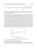
Figure 1 illustrates the modelled superstructure. All the possible alternative configurations and
interconnections between the three systems are embedded. The seawater feed passes through
a Sea Water Intake and Pre-treatment system (SWIP) where is chemically treated, according to
MSF and RO requirements. As Figure 1 shows, the feed stream of each process is not restricted
to seawater; instead, different streams can be blended to feed each system. Then, part of the
rejected stream leaving a system may enter into another one, even itself, resulting in a recycle.
The permeated streams of both RO systems and the distillate stream from MSF are blended to
produce the product stream, whose salinity is restricted to not exceed a maximum allowed salt
concentration. Furthermore, a maximum salt concentration is imposed for the blended stream
which is discharged back to the sea, in order to prevent negative ecological effects.


Fig. 1. Layout of the modelled superstructure
SWIP
Wfeed
msf
Wfeed
ro1
Wfeed
ro2
msf
F
W

ro2
F
W
MSF
HPP1
HPP2
RO1
RO2
msf
RM
W
ro1
Rro1
W
r
o
2
Rro2
W
msf
Rro2
W
msf
Rro1
W
msf
Rbdw
W
msf
P

W
ro1
Rro2
W
ro1
P
W
ro2
Rro1
W
ro2
P
W
ERS
ro1
Rbdw
W
ro2
Rbdw
W
ro1
RM
W
ro2
RM
W
PRODUCT
ro1
F
W

seawater
fresh water
brine
recycle
blow down
Optimization of Hybrid Desalination Processes
Including Multi Stage Flash and Reverse Osmosis Systems

313
Seawater characteristics: salt concentration and temperature are given data, as well as the
demand to be satisfied: total production and its maximum allowed salt concentration. On the
contrary, the flow rate of the seawater streams fed to each system are optimization variables,
as well as the flow rate and salt concentration of the product, blow down and inner streams.
The operating pressures for each RO system are also optimization variables. If the pressure
of the stream entering to a RO system is high enough, the corresponding high pressure
pumps are eliminated. Moreover, the number of modules operating in parallel at each RO
system is also determined by the optimization procedure. The remainder rejected flow rate
of both RO systems, if they do exist, will pass through an energy recovery system, before
being discharged back to the sea or fed into the MSF system.
For the MSF system, the geometrical design of the evaporator, the number of tubes in the
pre-heater, the number of flash stages, and others are considered as optimization variables.
The complete mathematical model is composed by four major parts: The Multi Stage Flash
model, The Reverse Osmosis model, network equations and cost equations. The following
section focuses on each of these four parts of the model.
3. Mathematical model
3.1 Multi Stage Flash model
The model representing the MSF system is based on the work (Mussati et al., 2004). A brief
description of the model is presented here.
The evaporator is divided into stages. Each stage has a seawater pheheater, a brine flashing
chamber, a demister and a distillate collector. Figure 2 shows a flashing stage.



Fig. 2. Scheme of flashing stage
In a MSF system, feed stream passes through heating stages and is heated further in the heat
recovery sections of each subsequent stage. Then, feed is heated even more using externally
suplied steam. After that, the feedwater passes through various stages where flashing takes
place. The vapor pressure at each stage is controlled in such way that the heated brine enters
each chamber at the proper temperature and pressure to cause flahs operation. The flash
vapor is drawn to the cooler tube bundle surfaces where it is condensed and collected as
distillate and paseses on from stage to stage parallelly to the brine. The distillate stream is
also flash-boiled, so it can be cooled and the surplus heat recovered for preheating the feed.
Figure 3 shows an scheme of a MSF system with NS stages.
Often, part of the brine leaving the last stage is mixed with the incoming feedwater because
it reduces the chemical pre-treatment cost. According to the interconections and
recirculations considered in the modeled superstructure, two typical MSF operating modes
are included: MSF-OT (without recycle) and MSF-BR (with recycle). However, more
complex configurations are also included, since different streams can be blended (at
different proportions) to feed the MSF system.
Brin
e
Brine flow
Demiste
r
Distillate tray
Tube bandle