Advances in Vibration Analysis Research Part 11 pot
Bạn đang xem bản rút gọn của tài liệu. Xem và tải ngay bản đầy đủ của tài liệu tại đây (2.85 MB, 30 trang )
A Plane Vibration Model for Natural Vibration Analysis of Soft Mounted Electrical Machines
289
stator orbit is shifted about 47° out of the horizontal axis. The semi-major axes of the orbits of
the bearing housings are shifted about 62° out of the horizontal axis. All orbits are still run
through forwards. In the 5th mode the semi-major axis of the orbit of the rotor mass is shifted
about 12° out of the vertical axis. The other orbits lie nearly in vertical direction. The stator
mass and the rotor mass oscillate out of phase to each other. The orbit of the stator mass and
the orbits of the bearing housing are run through forwards, while the orbit of the rotor mass
and the orbits of the shaft journals are run through backwards. In the 6th mode the semi-major
axes of the orbits of the stator mass and of the bearing housings are shifted about 80° out of the
vertical axis, while the semi-major axes of the orbits of the rotor mass and of the shaft journals
are shifted about 45° out of the vertical axis. All orbits are run through backwards.
Additionally the 6th mode shows a strong lateral buckling of the stator mass at the x-axis,
which leads to large orbits at the motor feet. Contrarily to the 1st mode the lateral buckling of
the stator mass is contrariwise to its horizontal movement, which means that if the stator mass
moves to the right the lateral buckling is to the left. To consider the influence of the foundation
damping on the natural vibrations, a simplified approach is used. Referring to (Gasch et al.,
2002), the damping ratio Df of the foundation can be described by the damping coefficients dfq,
stiffness coefficients cfq of the foundation and the stator mass ms, as a rough simplification.
dfq = Df ⋅ ms ⋅ 2 ⋅ c fq / ms with: q = z,y
(50)
The calculated natural frequencies and modal damping of each mode shape with and
without considering foundation damping are shown in Table 3. It is shown that considering
the foundation damping influences the natural frequencies only marginal, as expected. But
the modal damping values of some modes are strongly influenced by the foundation
damping. The modal damping values of the first two modes are strongly influenced by the
foundation damping, because the modes are nearly rigid body modes of the motor on the
foundation. Also the modal damping of the 6th mode is strongly influenced by the
foundation damping, because large orbits of the motor feet occur in this mode shape,
compared to the other orbits.
Modes
n
1
2
3
4
5
6
Without foundation damping (Df = 0)
With foundation damping (Df = 0.02)
Natural frequency Modal damping Natural frequency fn Modal damping
fn [Hz]
Dn [%]
[Hz]
Dn [%]
16.05
-0.11
16.05
0.95
25.35
0.51
25.33
1.84
35.22
65.75
35.23
65.72
37.72
6.97
37.67
7.36
48.50
3.39
48.54
4.24
52.63
1.0
52.61
4.17
Table 3. Natural frequencies and modal damping, motor mounted on a soft steel frame
foundation (cfz = 133 kN/mm; cfy = 100 kN/mm) with and without considering foundation
damping (Df = 0.02 and Df = 0), operating at rated speed (nN = 2990 r/min)
4.5.2 Critical speed map
Again, a critical speed map is derived to show the influence of the rotor speed on the natural
frequencies and the modal damping and to derive the critical speeds (Fig. 12).
290
Advances in Vibration Analysis Research
Ω / 2π
Natural frequency fn [Hz]
60
Mode 6
Mode 3
Mode 5
55
50
45
40
Mode 4
35
30
Mode 2
25
20
Mode 1
Note: The numbering of the modes is related
to the operation at rated speed (2990 r/min)
15
10
5
0
600
900
1200
1500
1800
2100
2400
2700
3000
3300
3600
3900
4200
4500
4800
Rotor speed nr [r/min]
75
70
Mode 3
Modal damping Dn [%]
65
60
15
≈
14
13
12
11
10
9
8
7
6
5
4
3
2
1
0
-1600
900
1200
-2
1500
1800
2100
2400
2700
3000
3300
3600
3900
4200
4500
4800
Mode 5
Mode 6
Mode 2
Mode 1
Mode 4
Rotor speed nr [r/min]
Fig. 12. Critical speed map, motor mounted on a soft steel frame foundation (cfz = 133
kN/mm; cfy = 100 kN/mm; Df =0.02)
Critical speed
1
2
3
4
5
Critical speed [r/min]
950
1540
2340
2900
3160
Modal damping Dn [%]
1.6
2.3
12.2
4.3
4.2
Table 4. Critical speeds, motor mounted on a soft steel frame foundation (cfz = 133 kN/mm;
cfy = 100 kN/mm; Df =0.02)
Fig. 12 shows that the limit of stability is here reached at about 4650 r/min, because the
modal damping of mode 4 gets zero at this rotor speed. For the rigid foundation the limit of
stability is already reached at a rotor speed of about 3900 r/min. But contrarily to the rigid
mounted motor here four critical speeds have to be passed before the operating speed (2990
r/min) is reached. Additionally a 5th critical speed is close above the operating speed. The
critical speeds and the modal damping in the critical speeds are shown in Table 4.
A Plane Vibration Model for Natural Vibration Analysis of Soft Mounted Electrical Machines
291
Table 4 shows that two critical speeds (4th and 5th) with low modal damping values are very
close to the operating speed (2990 r/min), having less than 5% separation margin to the
operating speed. Therefore resonance vibrations problems may occur. The conclusion is that
the arbitrarily chosen foundation stiffness values are not suitable for that motor with a
operation speed of 2990 r/min. To find adequate foundation stiffness values, a stiffness
variation of the foundation is deduced and a stiffness variation map is created (chapter
4.5.4). But preliminarily the influence of the electromagnetic stiffness on the natural
frequencies and modal damping values is investigated for the soft mounted motor.
Natural frequency fn [Hz]
4.5.3 Stiffness variation map regarding the electromagnetic stiffness
In this chapter the influence of the electromagnetic stiffness on the natural frequencies and
the modal damping values at rated speed is analyzed again, but now for the soft mounted
motor. Again the magnetic stiffness factor kcm is variegated in a range of 0….2 and the
influence on the natural frequencies and the modal damping values is analyzed. Fig. 13
55
53
51
49
47
45
43
41
39
37
35
33
31
29
27
25
23
21
19
17
15
Mode 6
Mode 5
Mode 4
Mode 3
Mode 2
Note: The numbering of the modes is related
to the magnetic stiffness factor kcm = 1
Mode 1
0
0,2
0,4
67
0,6
0,8
1
1,2
1,4
Magnetic stiffness factor kcm [-]
1,6
1,8
2
Modal damping Dn [%]
66
65
Mode 3
≈
8
Mode 4
7
6
5
Mode 5
4
Mode 6
3
2
Mode 2
1
Mode 1
0
0
0,2
0,4
0,6
0,8
1
1,2
1,4
1,6
1,8
2
Magnetic stiffness factor kcm [-]
Fig. 13. Stiffness variation map regarding the electromagnetic stiffness, motor mounted on a
soft steel frame foundation (cfz = 133 kN/mm; cfy = 100 kN/mm; Df = 0.02), operating at rated
speed (nN = 2990 r/min)
292
Advances in Vibration Analysis Research
shows that mainly the natural frequencies of the 4th mode and the 5th mode are influenced
by the magnetic spring constant. The natural frequencies of the other modes are hardly
influenced by the magnetic spring constant. The reason is that for the 4th mode and the 5th
mode the relative orbits between the rotor mass and the stator mass are large, compared to
the other orbits. Large orbits of the rotor mass and of the stator mass occur for these two
modes and both masses – the rotor mass and the stator mass – vibrate out of phase to each
other (Fig. 11), which lead to large relative orbits between these two masses. Therefore, the
electromagnetic interaction between these two masses is high and therefore a significant
influence of the magnetic spring constant on the natural vibrations occurs for these two
modes. In the 1st and 2nd mode the motor is acting like a one-mass system (Fig. 11) and
nearly no relative movements between rotor mass and stator mass occur. Therefore the
electromagnetic coupling between rotor and stator has nearly no influence on the natural
frequencies of the first two modes. The 3th mode is mainly dominated by large relative orbits
between the shaft journals and the bearing housings – compared to the other orbits – leading
to high modal damping. A relative movement between the rotor mass and the stator occurs,
but is not sufficient enough for a clear influence of the electromagnetic coupling. The 6th
mode is mainly dominated by large orbits of the motor feet, compared to the other orbits.
Again the relative movement of the stator and rotor is not sufficient enough that the
electromagnetic coupling influences the natural frequency of this mode clearly. The modal
damping values of all modes are only marginally influenced by the magnetic spring
constant, only a small influence on the modal damping of the 4th mode is obvious.
4.5.4 Stiffness variation map regarding the foundation stiffness
The foundation stiffness values cfz and cyz are changed by multiplying the rated stiffness
values cfz,rated and cfy,rated from Table 1 with a factor, called foundation stiffness factor kcf.
c fz = kcf ⋅ c fz,rated
(51)
Horizontal foundation stiffness: c fy = kcf ⋅ c fy,rated
(52)
Vertical foundation stiffness:
Therefore the vertical foundation stiffness cfz and the horizontal foundation stiffness cfy are
here changed in equal measure by the foundation stiffness factor kcf. The influence of the
foundation stiffness at rated speed on the natural frequencies and on the modal damping is
shown in Fig. 14.
It is shown that for a separation margin of 15% between the natural frequencies and the
rotary frequency Ω/2π the foundation stiffness factor kcf has to be in a range of 2.5…3.0. If
the foundation stiffness factor is smaller than 2.5 the natural frequency of the 5th mode gets
into the separation margin. If the foundation stiffness factor is bigger than 3.0 the natural
frequency of the 4th mode gets into the separation margin. Both modes – 4th mode and 5th
mode – have a modal damping less than 10% in the whole range of the considered
foundation stiffness factor (kcf = 0.5…4). Because of the low modal damping values of these
two modes, the operation close to the natural frequencies of these both modes suppose to be
critical. Therefore the first arbitrarily chosen foundation stiffness values (cfz,rated = 133
kN/mm; cfy,rated = 100 kN/mm) have to be increased by a factor of kcf = 2.5…3.0. With the
increased foundation stiffness values the foundation can still be indicated as a soft
foundation, because the natural frequencies of the 1st mode and the 2nd mode – the mode
A Plane Vibration Model for Natural Vibration Analysis of Soft Mounted Electrical Machines
293
Natural frequency fn [Hz]
shapes are still the same as in Fig. 11 – are still low, lying in a range between 24 Hz and 26
Hz for the 1st mode and between 33 Hz and 35 Hz for the 2nd mode.
⎧≤ 0.85 ⋅ Ω / 2π
Range of the foundation stiffness
fn ⎨
factor kcf for the boundary condition: ⎩≥ 1.15 ⋅ Ω / 2π
110
105
100
95
90
85
80
75
70
65
60
55
50
45
40
35
30
25
20
15
10
5
0
Mode 6
Separation margin of ±15%
to the rotary frequency Ω/2π
Mode 5
Ω / 2π
Mode 4
Mode 2
Mode 3
Mode 1
Note: The numbering of the modes is related
to the foundation stiffness factor kcf = 1
0,5
1
1,5
2
2,5
3
3,5
4
Foundation stiffness factor kcf [-]
75
70
Mode 3
Modal damping Dn [%]
65
60
10
≈
9
8
7
6
2
Mode 4
Mode 2
Mode 6
Mode 5
1
Mode 1
5
4
3
0
0,5
1
1,5
2
2,5
3
3,5
4
Foundation stiffness factor kcf [-]
Fig. 14. Stiffness variation map regarding the foundation stiffness, motor mounted on a soft
steel frame foundation, operating at rated speed (nN = 2990 r/min)
5. Conclusion
The aim of this paper is to show a simplified plane vibration model, describing the natural
vibrations in the transversal plane of soft mounted electrical machines, with flexible shafts
and sleeve bearings. Based on the vibration model, the mathematical correlations between
the rotor dynamics and the stator movement, the sleeve bearings, the electromagnetic and
the foundation, are derived. For visualization, the natural vibrations of a soft mounted 2pole induction motor are analyzed exemplary, for a rigid foundation and for a soft steel
frame foundation. Additionally the influence of the electromagnetic interaction between
rotor and stator on the natural vibrations is analyzed. Finally, the aim is not to replace a
294
Advances in Vibration Analysis Research
detailed three-dimensional finite-element calculation by a simplified plane multibody
model, but to show the mathematical correlations based on a simplified model.
6. References
Arkkio, A.; Antila, M.; Pokki, K.; Simon, A., Lantto, E. (2000). Electromagnetic force on a
whirling cage rotor. Proceedings of Electr. Power Appl., pp. 353-360, Vol. 147, No. 5
Belmans, R.; Vandenput, A.; Geysen, W. (1987). Calculation of the flux density and the
unbalanced magnetic pull in two pole induction machines, pp. 151-161, Arch.
Elektrotech, Volume 70
Bonello, P.; Brennan, M.J. (2001). Modelling the dynamic behaviour of a supercritcial rotor
on a flexible foundation using the mechanical impedance technique, pp. 445-466,
Journal of sound and vibration, Volume 239, Issue 3
Gasch, R.; Nordmann, R. ; Pfützner, H. (2002). Rotordynamik, Springer-Verlag, ISBN 3-54041240-9, Berlin-Heidelberg
Gasch, R.; Maurer, J.; Sarfeld W. (1984). The influence of the elastic half space on stability
and unbalance of a simple rotor-bearing foundation system, Proceedings of
Conference Vibration in Rotating Machinery, pp. 1-11, C300/84, IMechE, Edinburgh
Glienicke, J. (1966). Feder- und Dämpfungskonstanten von Gleitlagern für Turbomaschinen und
deren Einfluss auf das Schwingungsverhalten eines einfachen Rotors, Dissertation,
Technische Hochschule Karlsruhe, Germany
Holopainen, T. P. (2004) Electromechanical interaction in rotor dynamics of cage induction motors,
VTT Technical Research Centre of Finland, Ph.D. Thesis, Helsinki University of
Technology, Finland
Kellenberger, W. (1987) Elastisches Wuchten, Springer-Verlag, ISBN 978-3540171232, BerlinHeidelberg
Lund, J.; Thomsen, K. (1987). Review of the Concept of Dynamic Coefficients for Fluid Film
Journal Bearings, pp. 37-41, Journal of Tribology, Trans. ASME, Vol. 109, No. 1
Lund, J.; Thomsen, K. (1978). A calculation method and data for the dynamics of oil
lubricated journal bearings in fluid film bearings and rotor bearings system design
and optimization, pp. 1-28, Proceedings of Conference ASME Design and Engineering
Conference, ASME , New York
Schuisky, W. (1972). Magnetic pull in electrical machines due to the eccentricity of the rotor,
pp. 391-399, Electr. Res. Assoc. Trans. 295
Seinsch, H-O. (1992). Oberfelderscheinungen in Drehfeldmaschinen, Teubner-Verlag, ISBN 3519-06137-6, Stuttgart
Tondl, A. (1965). Some problems of rotor dynamics, Chapman & Hall, London
Vance, J.M.; Zeidan, F. J.; Murphy B. (2010). Machinery Vibration and Rotordynamics, John
Wiley and Sons, ISBN 978-0-471-46213-2, Inc. Hoboken, New Jersey
Werner, U. (2010). Theoretical vibration analysis of soft mounted electrical machines
regarding rotor eccentricity based on a multibody model, pp. 43-66, Springer,
Multibody System Dynamics, Volume 24, No. 1, Berlin/Heidelberg
Werner, U. (2008). A mathematical model for lateral rotor dynamic analysis of soft mounted
asynchronous machines. ZAMM-Journal of Applied Mathematics and Mechanics, pp.
910-924, Volume 88, No. 11
Werner, U. (2006). Rotordynamische Analyse von Asynchronmaschinen mit magnetischen
Unsymmetrien, Dissertation, Technical University of Darmstadt, Germany, ShakerVerlag, ISBN 3-8322-5330-0, Aachen
15
Time-Frequency Analysis for
Rotor-Rubbing Diagnosis
Eduardo Rubio and Juan C. Jáuregui
CIATEQ A.C., Centro de Tecnología Avanzada
Mexico
1. Introduction
Predictive maintenance by condition monitoring is used to diagnose machinery health.
Early detection of potential failures can be accomplished by periodic monitoring and
analysis of vibrations. This can be used to avoid production losses or a catastrophic
machinery breakdown. Predictive maintenance can monitor equipments during operation.
Predictions are based on a vibration signature generated by a healthy machine. Vibrations
are measured periodically and any increment in their reference levels indicates the
possibility of a failure.
There are several approaches to analyze the vibrations information for machinery diagnosis.
Conventional time-domain methods are based on the overall level measurement, which is a
simple technique for which reference charts are available to indicate the acceptable levels of
vibrations. Processing algorithms have been developed to extract some extra features in the
vibrations signature of the machinery. Among these is the Fast Fourier Transforms (FFT)
that offers a frequency-domain representation of a signal where the analyst can identify
abnormal operation of the machinery through the peaks of the frequency spectra. Since FFT
cannot detect transient signals that occur in non-stationary signals, more complex analysis
methods have been developed such as the wavelet transform. These methods can detect
mechanical phenomena that are transient in nature, such as a rotor rubbing the casing of a
motor in the machine. This approach converts a time-domain signal into a time-frequency
representation where frequency components and structured signals can be localized. Fast
and efficient computational algorithms to process the information are available for these
new techniques.
A number of papers can be found in the literature which report wavelets as a vibration
processing technique. Wavelets are multiresolution analysis tools that are helpful in
identifying defects in mechanical parts and potential failures in machinery. Multiresolution
has been used to extract features of signals to be used in classifications algorithms for
automated diagnosis of machine elements such as rolling bearings (Castejón et al., 2010;
Xinsheng & Kenneth, 2004). These elements produce clear localized frequencies in the
vibration spectrum when defects are developing. However, a more complex phenomena
occurs when the rotor rubs a stationary element. The impacts produce vibrations at the
fundamental rotational frequency and its harmonics, and additionally yield some high
frequency components, that increase as the severity of the impacts increases (Peng et al.,
2005).
Rotor dynamics may present light and severe rubbing, and both are characterized by a
different induced vibration response. It is known that conditions that cause high vibration
296
Advances in Vibration Analysis Research
levels are accompanied by significant dynamic nonlinearity (Adams, 2010). The resonance
frequency is modified because of the stiffening effect of the rubbing on the rotor (Abuzaid et
al., 2009). These systems are strongly nonlinear and techniques have been applied for
parameter identification. These techniques have developed models that explain the jump
phenomenon typical of partial rub (Choi, 2001; Choi, 2004).
The analysis of rubbing is accomplished with the aid of the Jeffcott rotor model for lateral
shaft vibrations. This model states the idealized equations of rotor dynamics (Jeffcott, 1919).
Research has been done to extend this model to include the nonlinear behavior of the rotor
system for rubbing identification. It has been shown that time-frequency maps can be used
to analyze multi-non-linear factors in rotors. They also reveal many complex characteristics
that cannot be discovered with FFT spectra (Wang et al., 2004). Other approaches use
analytical methods for calculating the nonlinear dynamic response of rotor systems. Secondorder differential equations which are linear for non-contact and strongly nonlinear for
contact scenarios have been used (Karpenko et al., 2002). Rub-related forces for a rotor
touching an obstacle can be modeled by means of a periodic step-function that neglects the
transient process (Muszynska, 2005).
In this chapter the phenomenon of rotor rubbing is analyzed by means of a vibrations
analysis technique that transforms the time-domain signal into the time-frequency domain.
The approach is proposed as a technique to identify rubbing from the time-frequency
spectra generated for diagnostic purposes. Nonlinear systems with rotating elements are
revised and a nonlinear model which includes terms for the stiffness variation is presented.
The analysis of the signal is made through the wavelet transform where it is demonstrated
that location and scale of transient phenomena can be identified in the time-frequency maps.
The method is proposed as a fast diagnostic technique for rapid on-line identification of
severe rubbing, since algorithms can be implemented in modern embedded systems with a
very high computational efficiency.
2. Nonlinear rotor system with rubbing elements
Linear models have intrinsic limitations describing physical systems that show large
vibration amplitudes. Particularly, they are unable to describe systems with variable
stiffness. To reduce the complexity of nonlinear problems, models incorporate simplified
assumptions, consistent with the physical situation, that reduce their complexity and allow
representing them by linear expressions. Although linearized models capture the essence of
the problem and give the main characteristics of the dynamics of the system, they are unable
to identify instability and sudden changes. These problems are found in nonlinear systems
and the linear vibration theory offers limited tools to explain the complexity of their
unpredictable behavior. Therefore, nonlinear vibration theories have been developed for
such systems.
The steady state response of the nonlinear vibration solution exhibits strong differences with
respect to the linear approach. One of the most powerful models for the analysis of
nonlinear mechanical systems is the Duffing equation. Consider the harmonically forced
Duffing equation with external excitation:
φ
(1)
Curves of response amplitude versus exciting frequency are often employed to represent
this vibration behavior as shown in Fig. 1. The solid line in this figure shows the response
Time-Frequency Analysis for Rotor-Rubbing Diagnosis
297
curve for a linear system. The vertical line at ω/ωn=1 corresponds to the resonance. At this
point vibration amplitude increases dramatically and it is limited only by the amount of
damping in the system. It is important to ensure that the system operates outside of this
frequency to avoid excessive vibration that can result in damage to the mechanical parts. In
linear systems amplitude of vibrations grows following a straight line as excitation force
increases.
Fig. 1. Resonant frequency dependency in nonlinear systems
In nonlinear systems the motion follows a trend that is dependent upon the amplitude of the
vibrations and the initial conditions. The resonance frequency is a function of the excitation
force and the response curve does not follow a straight line. When the excitation force
increases, the peak amplitude “bends” to the right or left, depending on whether the
stiffness of the system hardens or softens. For larger amplitudes, the resonance frequency
decreases with amplitude for softening systems and increases with amplitude for hardening
systems. The dashed lines in Fig. 1 show this effect.
When the excitation force is such that large vibration amplitudes are present, an additional
“jump” phenomenon associated with this bending arises. This is observed in Fig. 2. Jump
phenomenon occurs in many mechanical systems. In those systems, if the speed is increased
the amplitude will continue increasing up to values above 1.6ωn.
Fig. 2. Jump phenomenon typical of nonlinear systems
298
Advances in Vibration Analysis Research
When the excitation force imposes low vibration amplitudes, or there is a relative strong
damping, the response curve is not very different from the linear case as it can be observed
in the two lower traces. However, for large vibration amplitudes the bending effect gets
stronger and a “jump” phenomenon near the resonance frequency is observed. This
phenomenon may be observed by gradually changing the exciting frequency ω while
keeping the other parameters fixed. Starting from a small ω and gradually increasing the
frequency, the amplitude of the vibrations will increase and follow a continuous trend.
When frequency is near resonance, vibrations are so large that the system suddenly exhibits
a jump in amplitude to follow the upper path, as denoted with a dashed line in Fig. 2. When
reducing the excitation frequency the system will exhibit a sudden jump from the upper to
the lower path. This unusual performance takes place at the point of vertical tangency of the
response curve, and it requires a few cycles of vibration to establish the new steady-state
conditions.
There is a region of instability in the family of response curves of a nonlinear system where
such amplitudes of vibration cannot be established. This is shown in Fig. 3. It is not possible
to obtain a particular amplitude in this region by forcing the exciting frequency. Even with
small variations the system is unable to restore the stable conditions. Therefore, from the
three regions depicted in this figure, only the upper and lower amplitudes of vibration exist.
The same applies for a hardening system but with the peaks of amplitude of vibrations
bending to the right.
A rotor system with rub impact is complex and behaves in a strong nonlinearity. A
complicated vibration phenomenon is observed and the response of the system may be
characterized by the jump phenomena at some frequencies. Impacts are associated with
stiffening effects; therefore, modeling of rotor rub usually includes the nonlinear term of
stiffness.
When the rotor hits a stationary element, it involves several physical phenomena, such as
stiffness variation, friction, and thermal effects. This contact produces a behavior that
worsens the operation of the machine. Rubbing is a secondary transient phenomenon that
arises as a result of strong rotor vibrations. The transient and chaotic behavior of the rotor
impacts generate a wide frequency bandwidth in the vibrational response.
Fig. 3. Region of instability
Dynamics of the rotor rubbing can be studied with the Jeffcott rotor model (Jeffcott, 1919).
This model was developed to analyze lateral vibrations of rotors and consists of a centrally
Time-Frequency Analysis for Rotor-Rubbing Diagnosis
299
mounted disk on a flexible shaft. Rigid bearings support the ends of the shaft as shown in
Fig. 4. The model is more representative of real rotor dynamics for the inclusion of a
damping force proportional to the velocity of the lateral motion. The purpose of this model
was to analyze the effect of unbalance at speeds near the natural frequency, since the
vibration amplitude increase considerably in this region.
Fig. 4. Diagram of a rotor rubbing with a stationary element
Modifying the Jeffcott´s model, the rubbing phenomenon can be studied. A stationary
element can be added to the model to take rubbing into consideration. A diagram of the
forces that are involved during the rub-impact phenomenon is shown in Fig. 5.
Fig. 5. A Jeffcott rotor model with rubbing
At the contact point, normal and tangential forces are described by the following
expressions:
(2)
(3)
Where K R is the combined stiffness of the shaft and the contact stiffness.
This is valid for
(4)
300
Advances in Vibration Analysis Research
otherwise
0
(5)
For a Cartesian coordinate system forces are represented as:
φ
φ
(6)
φ
φ
(7)
And the motion equations of the rotor system are described by:
(8)
(9)
Where K is the stiffness of the system and C is the damping coefficient of the system.
The contact of the rotor with the stationary element creates a coupling of the system that
and the model becomes
causes a variation in the stiffness because of the non-continuous
nonlinear. The rotor rubs the element only a fraction of the circumferential movement and
the stiffness value varies with respect to the rotor angular position.
The nonlinear behavior can be related to the stiffness variation. As shown in Fig. 6, the
system´s stiffness can be related to the shaft stiffness KS, and it increases to KR during
contact. This increment can be estimated using the Hertz theory of contact between two
elastic bodies placed in mutual contact.
Fig. 6. Stiffness increase during contact
Assuming that the system´s stiffness can be represented as a rectangular function, then the
stiffness variation can be approximated as a Taylor series such that
(10)
3. Vibrations analysis with data-domain transformations
The vibrational motion produced by a rotating machine is complicated and may be analyzed
by transforming data from the time-domain to the frequency-domain by means of the
301
Time-Frequency Analysis for Rotor-Rubbing Diagnosis
Fourier Transform. This transform gives to the operator additional information from the
behavior of the machine that a signal in time-domain cannot offer.
Fourier developed a theory in which any periodic function f(t), with period T, can be
expressed as an infinite series of sine and cosine functions of the form:
(11)
2
Where ω denotes the fundamental frequency and 2ω, 3ω, etc., its harmonics. This series is
known as the Fourier series expansion and an and bn are called the Fourier coefficients. By
this way, a periodic waveform can be expanded into individual terms that represent the
various frequency components that make up the signal. These frequency components are
integer multiples of ω.
The following identity can be used to extend the Fourier series to complex functions:
(12)
(13)
Where cn can be obtained by the following integration:
1
2
(14)
This applies to periodic functions on a 2π interval.
Fourier series can be extended to functions with any period T with angular frequency
ω=2π/T. Sine and cosine functions have frequencies that are multiples of ω as in Eq. (11).
For non-periodic functions, with period T, discrete frequencies nω separated by Δω=2π/T,
and taking the limit as T→∞, nΔω becomes continuous and the summation can be expressed
as an integral. As a result, the continuous Fourier transform for frequency domain is defined
as:
(15)
While for time domain the inverse Fourier transform is defined as:
1
2
(16)
And f=f(t) satisfying the condition
|
|
∞
(17)
Since computers can’t work with continuous signals, the Discrete Fourier Transform (DFT)
was developed and implemented through the Fast Fourier Transform (FFT). The FFT is a
fast algorithm for computing the DFT that requires the size of the input data to be a power
302
Advances in Vibration Analysis Research
of 2. FFT is a helpful engineering tool to obtain the frequency components from stationary
signals. However, non-stationary phenomena can be present in signals obtained from real
engineering applications, and are characterized by features that vary with time.
A difficulty that has been observed with FFT is that the complex exponentials used as the
basis functions have infinite extent. Therefore, localized information is spread out over the
whole spectrum of the signal. A different approach is required for this type of signals.
Time-frequency methods are used for their analysis and one of the most used methods is the
Short Time Fourier Transform (STFT). This was the first time-frequency technique
developed. The solution approach introduces windowed complex sinusoids as the basis
functions.
The STFT is a technique that cuts out a signal in short time intervals, which can be assumed
to be locally stationary, and performs the conventional Fourier Transform to each interval.
In this approach a signal
is multiplied by a window function
, centered at , to
obtain a modified signal that emphasises the signal characteristics around :
1
2
(18)
Frequency distribution will be reflected around after applying the Fourier Transform to
this window. The spectral density of the energy at time can be written as follows:
,
|
|
1
2
(19)
As expected, a different spectrum will be obtained for each time. A Spectrogram, which is
the time-frequency distribution, can be constructed with the resulting spectra. Resolution in
time and frequency depends on the width of the windows
. Large windows will provide
a good resolution in the frequency domain, but poor resolution in time domain. Small
windows will provide good resolution in time domain, but poor resolution in frequency
domain. The major disadvantage of this approach is that resolution in STFT is fixed for the
entire time-frequency map. This means that a single window is used for all the frequency
analysis. Therefore, only the signals that are well correlated in the time interval and
frequency interval chosen will be localized by the procedure. It may be thought of as a
technique to map a time-domain signal into a fixed resolution time-frequency domain.
This drawback can be surpassed with basis functions that are short enough to localize high
frequency discontinuities in the signal, while long ones are used to obtain low frequency
information. A new transform called wavelet transform achieves this with a single
prototype function that is translated and dilated to get the required basis functions.
The wavelet transform is a time-frequency representation technique with flexible time and
frequency resolution. Conversely to the STFT where the length of the windows function
remains constant during the analysis, in the wavelet approach a function called the mother
wavelet is operated by translation and dilation to build a family of window functions of
variable length:
ψ
1
√
ψ
(20)
Where ψ(t) is the mother wavelet function, the scale parameter, and the time shift or
dilation parameter. Based on the mother wavelet function, the wavelet transform is defined as:
303
Time-Frequency Analysis for Rotor-Rubbing Diagnosis
ψ
,
ψ
(21)
, are the wavelet coefficients.
And ψ
The wavelet transform is different from other techniques in that it is a multiresolution signal
analysis technique that decomposes a signal in multiple frequency bands. By operating over
and the wavelets permit to detect singularities, which makes it an important technique
for nonstationary signal analysis.
Due to this characteristic, the wavelet transform is the analysis technique that we found
more suitable for the analysis of the rubbing phenomenon.
4. Experimental methodology
An experimental test rig was implemented to get a deeper understanding of the main
characteristics of the rubbing phenomenon, and to apply the wavelet analysis technique in
the processing and identification of the vibrations produced by the rub-impact of the
system. Elements were included to run experiments under controlled conditions. Fig. 7
shows the experimental set-up.
Fig. 7. Test rig for the rubbing experiments
The experimental system is composed of a shaft supported by ball bearings and coupled to
an electrical motor with variable rotational speed. The velocity of the motor was controlled
with an electronic circuit. A disk was installed in the middle of the shaft, which was drilled
to be able to mount bolts of different masses to simulate unbalance forces. An adjustable
mechanism was designed in order to simulate the effect of a rotor rubbing a stationary
element. The position of the device, acting as the stationary element, was adjusted with a
threaded bolt that slides a surface to set the clearance between the rotating disk and the
rubbing surface. The shaft and disk were made of steel, and the rubbing device of
aluminium alloy. Light and severe rubbing were simulated by controlling the speed of the
rotor. Low velocities caused light rubbing while high velocities generated severe impact-like
rubbing vibrations. Both types of rubbing were analyzed with the proposed methodology.
An accelerometer was used to measure the vibrations amplitude. Output of the
accelerometer was connected to a data acquisition system to convert analog signals to digital
data with a sampling rate of 10 kHz. An antialias filter stage was included to get a band
limited input signal.
Experimental runs were carried out for fixed and variable rotor velocities. Fixed velocities
were tested for values between 350 rpm and 1900 rpm. Continuous variable velocity
experiments were also carried out to simulate a rotor system under ramp-up and rampdown conditions, to verify the preservation of the scale and temporal information with the
processing technique used.
304
Advances in Vibration Analysis Research
Daubechies 4 wavelet transform was implemented to convert the signal from the
time-domain to the time-frequency domain. Scaling and wavelet functions for this transform
are shown in Fig. 8.
1
SCALING FUNCTION
0.5
WAVELET FUNCTION
0
-0.5
0
0.25
0.5
0.75
1
Fig. 8. Daubechies D4 scaling and wavelet functions
Implementation of the continuous wavelet transform is impractical, especially for on-line
detection devices for process monitoring purposes. This implementation consumes a
significant amount of time and resources. An algorithm for the discrete wavelet transform
(DWT) is used to overcome this situation. It is based on a sub-band coding which can be
programmed with a high computational efficiency. Subband coding is a multiresolution signal
processing technique that decomposes the signal into independent frequency subbands.
With this approach, the DWT applies successive low-pass and high-pass filters to the
discrete time-domain signal as shown in Fig. 9. This procedure is known as the Mallat
algorithm.
Fig. 9. Algorithm for the sub-band decomposition of the input signal
The algorithm uses a cascade of filters to decompose the signal. Each resolution has its own
pair of filters. A low-pass filter is associated with the scaling function, giving the overall
picture of the signal or low frequency content, and the high-pass filter is associated with the
wavelet function, extracting the high frequency components or details. In Fig. 9 the low-pass
filter is denoted by H and the high-pass filter is denoted by G. Each end raw is a level of
decomposition. A sub-sampling stage is added to modify the resolution by two at each step
of the procedure. As a result of this process, time resolution is good at high frequencies,
while frequency resolution is good at low frequencies.
Time-Frequency Analysis for Rotor-Rubbing Diagnosis
305
For each transform iteration the scale function to the input data is applied through the lowpass and high-pass filters. If the input array has N cells, after applying the scale function, the
down-sampling by two, which follows the filtering, halves the resolution and an array with
N/2 values will be obtained. With the low-pass branch, coarse approximations are obtained.
The high-pass filtered signal will reflect the fluctuations or details content of the signal. By
iterating recursively a signal is decomposed into sequences. The successive sequences are
lower resolution versions of the original data.
The implemented form of the Daubechies 4 wavelet transform has a wavelet function with
four coefficients and a scale function with four coefficients. The scale function is:
(22)
Where scaling coefficients are defined as
1
√3
4√2
3
√3
4√2
3
√3
4√2
1
√3
4√2
(23)
(24)
(25)
(26)
The wavelet function is:
(27)
Where wavelet coefficients are defined as
(28)
(29)
(30)
(31)
Each wavelet and function value is calculated by taking the product of the coefficients with
four data values of the input data array. The process is iterated until desired results are
reached.
5. Experimental results and discussion
The methodology described in the previous section was applied and experimental runs
were carried out with the aid of the test rig to obtain a deeper comprehension of the rubbing
phenomenon. Fig. 10 shows results for time and frequency domains for the rotor rubbing
306
Advances in Vibration Analysis Research
and no-rub experimental runs. The upper row corresponds to time-domain signals, while
the lower row shows the frequency-domain signals.
With no-rub (upper left), the signal in time-domain is characterized by a uniform trace with
a small dispersion of data produced by the low-level noise of the measuring system.
However, when rub occurs (upper right), as acceleration is the measurement engineering
unit, even for low level rubbing the energy content of the signal is high, and spikes appear
at the location of each rub-contact.
The spectral distribution of the signal obtained when the rotor is rubbing shows the wide
frequency bandwidth in the vibrational response, produced by the chaotic behavior of the
rubbing phenomenon.
Fig. 10. Spectral distribution of the vibrations for the rotor rubbing and no-rubbing
When rubbing is present, the response is dependent on the angular frequency of the rotor.
For low rotor velocities rub generates low vibration amplitudes as shown in the acceleration
values in the upper graph of Fig. 11. This can be considered a light-rubbing, but when the
rotor velocity is high, the time-domain response of the vibrations produced is quite different
and get closer to an impact response characterized by spikes with high acceleration values.
This response can be seen in the lower graph of Fig. 11. The amplitudes of vibrations for
light rubbing are within ±0.1 g, while for severe rubbing peak values reach ±1 g, about ten
times higher.
Processing results of the signals for the rotor with rubbing and without rubbing to obtain
the spectral distribution are shown in Fig. 12. The graph localizes the natural frequency of
Time-Frequency Analysis for Rotor-Rubbing Diagnosis
307
the test rig for both cases. As explained in the introductory section, the nonlinear nature of
the system produced a slight different vibrations pattern when rubbing is present. Solid line
shows the natural frequency for the rub-free experiments. However, the dotted line
corresponds to the experiments with rubbing induced to the rotor, and as expected there is a
shift in the natural frequency.
Fig. 11. Vibrations amplitude for light rubbing and severe rubbing
Frequency shift occurs to the right, with the trend to move to the high frequency side of the
spectrum, which means that the system is hardening as a result of the stiffness increase
produced by the contact of the rotor with the stationary element. The amplitude of the
natural frequency also increases as a product of the higher energy content of the
rub-impacts.
The signal of the vibrations was processed to transform the data from the time-domain to
the time-frequency domain. Wavelet transform Daubechies 4 was used for the
transformation and results are shown in Fig. 13.
As stated before, a vector is obtained with this procedure which is the same size as the
original vector. Recalling the subband coding, upper half of the vector contains the high
frequency content of the information (subband 1). From the remaining data, upper half
contains the next subband with mid-frequency content (subband 2), and so on. This way, the
low frequency content of the information is coded and located in the lower part of the vector
while the high frequency content is coded into the higher indexes of the vector. Indexes
308
Advances in Vibration Analysis Research
represent the transformed values in the resulting vector which amplitude is a function of the
correlation between the input signal and the mother wavelet. A higher value for the index
means a stronger correlation and therefore a major content of that frequency corresponding
to a particular value of scale and translation.
Fig. 12. Resonance frequency dependence observed for a rotor with rubbing
Taking this into consideration, it can be observed that for light rubbing the correlation gets
stronger for mid-value indexes, which means that light rubbing is characterized by
frequencies that fall in the lower middle of the frequency spectrum.
On the other side, rub-impacts produced by the contact of the rotor with the stationary
element at high rotational frequencies, are characterized by spikes with a high frequency
content. The wavelet transformation enhances this type of rubbing as can be observed in the
upper half of the vector for severe rubbing shown in Fig. 13 (subband 1), although some
rubbing information can be found in the next subband. As both light and severe rubbing
may be present in a rotor, the sum of the frequency content produced by the phenomena
reflects again a wide spectral distribution in the vibrational response.
To test the wavelet approach as a rubbing detection technique, especially for severe rubbing
where it is desirable to assess alert signals before a catastrophic failure occurs as it can
happens under some rubbing conditions, a vibration signal which presents rub-impacts was
chosen. The test data are shown in Fig. 14.
There are two spikes in the graph produced by the rotor rubbing at high velocity rotation.
These spikes can be treated as singularities of transient nature whose occurrence cannot be
predicted. A technique like wavelets that analyzes a signal by comparison of a basis wavelet
that is scaled and translated to extract frequency and location information is ideal for this
situation. The procedure enhances these singularities and makes it easier their detection as it
is demonstrated next.
Time-Frequency Analysis for Rotor-Rubbing Diagnosis
Fig. 13. Rotor rubbing signal transformed to time-frequency domain with wavelets
Fig. 14. Time-domain vibrations with rub-impact
309
310
Advances in Vibration Analysis Research
Graphs showing the details of the impacts are shown in Fig. 15. The signal is characterized
by a sudden excitation that generates a mechanical oscillation that grows to peak amplitude
and decays as the impact energy dissipates. Each impact is characterized by only a few
cycles that analyzed with the traditional FFT would not have enough energy to obtain a
clear spectral definition.
Fig. 15. Details of the transient impacts analyzed
A wavelet decomposition of this signal was made and the main subbands are shown in
Fig. 16. Subbands are associated with their corresponding frequency range according to the
sampling rate established during the experiments. The graph shows the frequency content
between 78 Hz and 5 kHz.
From this graph it is observed that the subband with the higher frequency content
encompasses the information of the transient signals. The correlation technique enhances
the spikes giving amplitude values higher than the coefficients where impacts are not
present. This makes it easier to establish a discrimination criterion and an estimation of their
values to determine the presence and severity of the rubbing for diagnostic purposes.
Additionally, as the transient signals produced are in the first subband, only the first level of
decomposition in the wavelet transformation is necessary reducing the computing time that
it takes to make the analysis and optimizing the detection process.
The experimental results of the vibrations presented in the previous discussion were
analyzed through one of the approaches that wavelets offer to the vibration analyst. This is a
time-frequency representation of the data from which it can be extracted the information of
interest to apply the necessary processes and criteria for the rubbing detection. This
approach permits the characterization of the signal from which it can be obtained the
necessary information for the implementation of the technique for the design of testing
equipment with automatic detection and recognition of the rubbing phenomena.
Another type of representation of the information that wavelets offer are the time-frequency
maps. These are contour plots where the wavelet coefficient values are plotted against the
time and scale parameter, that is, translation and frequency. One axis represents time, the
other axis frequency, and the amplitude of the vibrations is color-coded. The contour maps
permit to visualize the whole picture of the frequencies present in the signal as well as their
occurrence or location in time.
Time-Frequency Analysis for Rotor-Rubbing Diagnosis
311
Fig. 16. Subband coding with wavelets of the vibrational response with impact-rubbing
The light rubbing data was processed with commercially available software by means of the
Morlet continuous wavelet transform and results are shown in Fig. 17. In this graph, the
color coding is red for low amplitude vibrations throughout blue for high amplitude
vibrations. It can be observed the intermittent nature of the rubbing and, in concordance
with Fig. 13, that the main vibrations are limited to frequencies below 1 250 Hz.
An analogous process was applied to severe rubbing data and results are shown in Fig. 18.
The image shows that mid-range frequencies get stronger while high frequencies appear as
a result of the increase in the vibrations amplitude as in the lower graph of Fig. 13. Upper
spots in the time-frequency map (rub-impacts) appear elongated and lower spots stretched
due to the compromise between the time and frequency resolution of the technique as stated
in the introduction.
Additionally, an experimental run was carried out varying continuously the rotating
conditions to obtain a sweep from a low to a high velocity and then decreasing the velocity
until a minimum value. Results are shown in Fig. 19.
It can be seen that as time runs throughout the experiment, velocity increases and higher
frequency components appear. These components get their peak value near the middle of
the time axis where the maximum velocity is reached, and then begin to fade showing the
trend of the higher frequencies to disappear as velocity decreases. This graph confirms the
wide spectral bandwidth of the rubbing phenomena.
312
Advances in Vibration Analysis Research
Fig. 17. Time-Frequency map for light rubbing
It is important to notice the evolution of the frequencies as time passes by. There is an
unsteady variation of frequencies, and in Fig. 19 it can be seen how they have an
unsymmetrical pattern even with speed variations.
Fig. 18. Time-frequency map for severe rubbing
Time-Frequency Analysis for Rotor-Rubbing Diagnosis
313
Fig. 19. Time-frequency map for a run-up and run-down rotor velocity sweep
6. Conclusions
Rotor rubbing has been analyzed with a methodology that processes the vibrations signal in
such a way that time and scale information is preserved. It was demonstrated that with this
approach vibrations of transient nature can be studied through a controlled subband coding
scheme and time-frequency spectra. The technique revealed additional information that
traditional processing techniques cannot, such as FFT. Experimental results showed that
light rubbing presents a vibrational response characterized by a rich frequency content
spectrum, and that severe rubbing is more adequately described as an impact-like transient
behavior. Accordingly, impacts could be identified and localized with wavelets in the
upper-frequency subbands which resulted after the algorithm was applied.
Since rotor-to-stator contact changes the effective stiffness of the coupled elements, a
frequency shift was identified that shows the nonlinear response of the system. Timefrequency maps evidenced again the wide spectral response and differences between light
and severe rotor rubbing, and location in time of the rub-impacts. The processing algorithm
can be implemented with a high computational efficiency for on-line inspection systems for
continuous machinery condition monitoring.
7. References
Abuzaid, M.A. ; Eleshaky, M.E. & Zedan, M.G. (2009). Effect of partial rotor-to-stator rub on
shaft vibration. Journal of Mechanical Science and Technology, Vol. 23, No. 1, 170-182.
Adams, M.L. (2010). Rotating Machinery Vibration, 84, CRC Press, Taylor & Francis Group,
ISBN 978-1-4398-0717-0, Boca Raton, FL, USA.