21
Neurophysiological Correlate of
Binaural Auditory Filter Bandwidth and
Localization Performance Studied by
Auditory Evoked Fields
Yoshiharu Soeta and Seiji Nakagawa
National Institute of Advanced Industrial Science and Technology (AIST)
Japan
1. Introduction
Binaural hearing is specifically useful for our ability to separate a speech from a background
noise and localize sounds. Binaural hearing performances are influenced by binaural
auditory filter, inteaural time delay (ITD), interaural correlation (IAC), and so on. Some
psychological experiments have clarified binaural auditor filter bandwidths (Kollmeier &
Holube, 1989; Holube et al., 1998) and performance of sound localization related to ITD and
IAC (Mills, 1958; Jeffress et al., 1962). However, little is known about the neural correlates,
which makes an important contribution to our understanding of the auditory system.
Therefore, we tried to estimate binaural auditory filter bandwidth and localization
performance by the response in human auditory cortex.
Frequency selectivity has an important role in many aspects of auditory perception. For
example, one sound may be obscured or rendered inaudible in the presence of other sounds.
Frequency selectivity represents the ability of the auditory system to separate out or resolve
the frequency components of a complex sound and can be characterized by the auditory
filter bandwidths. Auditor filter bandwidths have been used to identify a fundamental
perceptual unit that defines the frequency resolution of the auditory system – the critical
bandwidth (CBW). The critical band (CB) concept has been used to explain a wide range of
perceptual phenomena involving complex sounds.
Physiological correlates of the CBW have been described in several studies examining the
auditory evoked potential (AEP) or auditory evoked field (AEF) in humans. Zerlin (1986)
reported an abrupt increase in the amplitude of wave V of the brainstem AEP responses
when the bandwidth of a two-tone complex approximated the CBW. Burrows & Barry
(1990) reported that the amplitude of Na of the AEP rapidly increased when the frequency

separation of a two-tone complex increased beyond the CBW. Soeta et al. (2005) and Soeta &
Nakagawa (2006a) found that the amplitude of the N1m of AEFs increased with increasing
the bandwidth of a bandpass noise or the frequency separation of a two-tone complex
increased beyond the CBW. These studies have focused on physiological correlates of the
monaural auditory filter in human auditory cortex; however, relatively little is known about
the physiological correlates of the binaural auditory filter in the human auditory cortex. In
natural listening environments, both the monaural and binaural auditory filters contribute
Advances in Sound Localization

388
to the performance of the auditory system in separating desired a speech from an undesired
background noise (Kollmeier & Holube, 1989). Therefore, the physiological correlates of the
binaural auditory filter in human auditory cortex merit investigation.
Performance of sound localization is also important in natural listening environments. There
are two possible cues as to the sound localization: an ITD and an interaural level difference
(ILD). Consider a sinusoidal sound source located to one side of the head in the horizontal
plane with an azimuth of 45º and an elevation of 0º. The sound reaching the farther ear is
delayed in time and is less intense than that reaching the nearer ear. Owing to the physical
nature of sounds, ITDs and ILDs are not equally effective at all frequencies (Moore, 2003). For
low-frequency tones, ITDs provide effective and unambiguous information about the location
of the sounds. However, for higher-frequency sounds, ITDs provide ambiguous cues. For
sinusoids, the physical cues of ILDs should be most useful at high frequencies, while the cues
of ITDs should be most useful at low frequencies. The idea that sound localization is based on
ILDs at high frequencies and ITDs at low frequencies has been called the “duplex theory.” The
minimum audible angle (MAA) for sinusoidal signals presented in the horizontal plane as a
function of frequency has been investigated previously (Mills, 1958). The resolution of
auditory space is measured in terms of the MAA, which is defined as the smallest detectable
difference between the azimuths of two identical sources of sound. Performance worsens
around 1500-1800 Hz. This is consistent with the duplex theory, which states that ITD
differences above 1500 Hz between the two ears are ambiguous cues for localization, while

ILDs up to 1800 Hz are small and do not change much with azimuth (Moore, 2003).
Physiological correlates of the localization performance related to ITDs is still unclear.
ITDs can be measured by the interaural cross-correlation function (IACF) between two
sound signals received at both the left and right ears. Whether there exist physiological
processes that correspond to IACF processes is an important question, and answers have
generally been sought in utilizing the so-called coincidence, or cross-correlation model for
the evaluation of ITD first proposed by Jeffress (1948). Numerous theories of the binaural
system rely on a coincidence detector or cross-correlator to act as a comparator element for
signals arriving at both ears (e.g., Webster, 1951; Sayers & Cherry, 1957; Jeffress et al., 1962;
Osman, 1971; Colbum, 1977; Lindemann, 1986; Joris et al., 1998). IAC can also be measured
by the IACF. The width of the sound image changes according to the IAC (Licklider, 1948;
Kurozumi & Ohgushi, 1983; Ando & Kurihara, 1986; Blauert & Lindemann, 1986). When
sounds are delivered dichotically, the sound image varies with the IAC of the sound. If the
IAC is high, the sound image is fused and occupies a narrow region. As the IAC decreases,
the sound becomes more diffuse. Localization performance has been previously measured
as a function of the degree of IAC (Jeffress et al., 1962; McEvoy et al., 1991; Zimmer &
Macaluso, 2005), and the results showed that localization performance decreases slowly as
the IAC is reduced especially below IAC ≈ 0.2.
Stimuli with ITDs have frequently been used in AEP and AEF studies of sound localization,
and the processes underlying sound source localization have been analyzed (Ungan et al.,
1989; McEvoy et al., 1990; Sams et al., 1993; McEvoy et al., 1993; 1994). The amplitude of
N1m has been found to decrease with decreasing contralaterally-leading ITD (McEvoy et al.,
1993; Sams et al., 1993). Magnetoencephalographic (MEG) research has benefited from the
recent development of headphone-based 3D-sound technology, including head-related
transfer functions, which are digital filters capable of reproducing the filtering effects of the
pinna, head, and body (Palomäki et al., 2000; Fujiki et al., 2002; Palomäki et al., 2002; 2005).
This research has found that the amplitude and latency of the N1m exhibits directional
Neurophysiological Correlate of Binaural Auditory Filter Bandwidth and
Localization Performance Studied by Auditory Evoked Fields


389
tuning to the sound location, with the amplitude of the right-hemisphere N1m being
particularly sensitive to the amount of spatial cues in the stimuli. However, the processes
underlying sound localization performance in the human auditory cortex have not been
analyzed yet.
Therefore, in order to clarify the processes underlying basic binaural hearings in human
auditory cortex, we investigated the physiological counterparts of binaural auditory filter
bandwidth as a function of frequency and localization performance related to ITD,
frequency, and IAC by AEFs.
2. Estimation of binaural auditory filter bandwidth
Some psychological experiments have examined whether monaural and binaural conditions
have the same auditory filter bandwidths, and differences between the monaural and
binaural conditions have been found (e.g., Kollmeier & Holube, 1989; Holube et al., 1998).
However, there is little evidence of the physiological correlates of the auditory filter
bandwidths under binaural listening conditions. Here, physiological counterparts to the
binaural auditory filter bandwidth in the human auditory cortex were examined by AEFs.
We tried to estimate the binaural auditory filter bandwidth as a function of frequency based
on the amplitudes of the N1m components, which is prominent, robust, and controlled by
the physical aspects of the stimulus (Näätänen & Picton, 1987).
The tone frequencies used in this experiment, f1 and f2, were geometrically centered on 125,
250, 500, 1000, 2000, 4000, and 8000 Hz. Frequency separations (f2-f1) were set at 2-160% of
the center frequency. The higher frequency tone (f2) was presented to the right ear and the
lower frequency tone (f1) was presented to the left ear. The duration of the stimuli used
during the experiments was 0.5 s, including cosine rise and fall ramps of 10 ms. Participants
were presented with stimuli dichotically at a sound pressure level (SPL) of 60 dB through
insert earphones (Etymotic Research ER-2, Elk Grove Village, Illinois, USA) with 29-cm
plastic tubes and eartips inserted into the ear canals. SPLs of all stimuli were checked with
an ear simulator (Brüel & Kjaer Ear Simulator Type 4157, Naerum, Denmark).
Eight right-handed participants (22-37 years) took part in the experiment. All had normal
audiological status and no history of neurological diseases. Informed consent was obtained

from each participant after the nature of the study was explained. The study was approved
by the Ethics Committee of the National Institute of Advanced Industrial Science and
Technology (AIST).
AEFs were recorded using a 122-channel whole-head MEG system (Neuromag-122
TM
;
Neuromag Ltd., Helsinki, Finland) in a magnetically shielded room (Hämäläinen et al.,
1993). Seven experimental sessions, each with a different center frequency, were carried out.
In each session, stimuli were presented in a randomized order with an interstimulus interval
selected at random from 1.0 to 1.5 s. To maintain a constant level of vigilance, participants
were instructed not to pay attention to sounds but to concentrate on a self-selected silent
movie projected on a screen in front of them. Magnetic data were sampled at 400 Hz after
being band-pass-filtered between 0.03 and 100 Hz, and then averaged approximately 100
times. Responses were rejected if the magnetic field exceeded 3000 fT/cm in any channel.
The averaged responses were digitally filtered between 1.0 and 30.0 Hz. The mean
amplitude of the pre-stimulus period of the 0.2 s was used as the baseline level.
Source analysis based on the model of a single moving equivalent current dipole (ECD) in a
spherical volume conductor was applied to the measured field distribution. Source
Advances in Sound Localization

390
estimates were based on a subset of 40-44 channels in the latency range of 70-130 ms over
each left and right temporal hemisphere. ECDs were found separately for the left and right
hemisphere data using a least-squares search (Hämäläinen et al., 1993). The amplitudes and
latencies of the dipole with the maximal goodness of fit were defined as the N1m
amplitudes and latencies for further analysis. Only dipoles with a goodness of fit of more
than 80% were included in further analyses. The dipole location and orientation were
determined in a head-based coordinate system with the origin set to the midpoint of the
medial-lateral axis (x-axis) between the entrances of the left and right ear canals. The
posterior-anterior axis (y-axis) was positioned through the nasion and the origin, and the

inferior-superior axis (z-axis) was positioned through the origin perpendicular to the x-y
plane.
Clear N1m responses were observed in both the right and left temporal regions in all
participants with all stimuli (Fig. 1). The N1m latencies were not significantly affected by
frequency separation and hemisphere with all center frequencies.
When the frequency separation was less than 10-20% of the center frequency, the N1m
amplitude was independent of the frequency separation. When the frequency separation
was more than about 10-20% of the center frequency, the N1m amplitude increased with
increasing frequency separation (Fig. 2). Thus, N1m amplitudes show CB-like behavior
under dichotic conditions. Regarding the increase in N1m amplitude above the CBW of the
dichotically presented two-tone frequencies, Yvert et al. (1998) showed that the N1m
amplitude increased with increasing frequency separation when the frequency separation


Fig. 1. Typical waveforms of AEFs in response to dichotically presented two-tones with
different frequency separations from 122 channels in one subject. The center frequency was
1000 Hz. The waveforms of the AEFs have different frequency separations.
Neurophysiological Correlate of Binaural Auditory Filter Bandwidth and
Localization Performance Studied by Auditory Evoked Fields

391

Fig. 2. Mean N1m amplitudes (± SEMs) from the right (z) and left ({) hemispheres as a
function of the frequency separation. The data have been fitted with the best combination of
two straight lines, one of zero slope for narrow frequency separations, and one of non-zero
slope, by the method of least squares. The intersection estimates the critical bandwidth.
Advances in Sound Localization

392
was more than 25% of the center frequency, which is consistent with the present finding.

These results indicate that each tone stimulates both left and right hemispheres, and that the
overall spectrum of the binaural stimulus becomes broader as the interaural frequency
difference increases. This in turn reduces the interference between ipsilateral and
contralateral pathways (binaural interaction) and activates many neurons in the auditory
cortex.


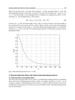
Fig. 3. The symbols () indicate the estimates of the binaural auditory filter bandwidth from
the N1m amplitudes at various center frequencies. The curve fitted to the data is specified
by the equation in the figure. For comparison, the dotted line and dash-dot line show the the
monaural CB function (Zwicker & Terhardt, 1980) and equivalent rectangular bandwidth of
the auditory filter (Moore & Glasberg, 1987), respectively.
We estimated the binaural auditory filter bandwidth by fitting the N1m amplitude as a
function of frequency separation with the best combination of two straight lines as shown
by the arrows in Fig. 2 in each center frequency. The averaged N1m amplitude from the left
and right hemispheres was used for this fitting, because the main effect of hemisphere on
the N1m amplitude was not significant. The estimated binaural critical bandwidth was
approximately 10-20% of the center frequency and fitted to an equation (Fig. 3). The
resulting function was 0.45f
2
+ 0.92f – 0.89 (Fig. 3). For comparison, the dotted line and dash-
dot line show the estimated monaural auditory filter bandwisth (Zwicker & Terhardt, 1980;
Moore & Glasberg, 1987). For the diotic condition, the effects of frequency separation of a
two-tone complex and a three-tone complex on the AEFs have also been examined when the
center frequency was 1000 Hz (Soeta & Nakagawa, 2006a). The auditory filter bandwidth
was estimated in a similar way to that used in this study; the estimated auditory filter
bandwidth was 153 Hz for a two-tone complex and 236 Hz for a three-tone complex. For the
monaural condition, Sams & Salmelin (1994) investigated the frequency tuning of the
human auditory cortex by masking tones using continuous white-noise maskers with
frequency notches at the tone frequencies. The estimated auditory filter bandwidth for 1000

Neurophysiological Correlate of Binaural Auditory Filter Bandwidth and
Localization Performance Studied by Auditory Evoked Fields

393
and 2000 Hz tones were 247 and 602 Hz, respectively. The reasons for these differing
bandwidths are unclear. One factor might be the influence of a different presentation of the
stimulus; that is, dichotic, diotic and monaural presentation. Additionally, different spectra
or temporal shapes of the stimulus may have contributed to the discrepancies. Finally,
different participants may have contributed to the discrepancies.
All eatimated ECDs were located at or near the Heschl’s gyrus or planum temporale. The
effects of frequency separation on the ECD locations of the N1m in each hemisphere and
each center frequency were statistically analyzed by a repeated-measure ANOVA. While
this analysis yielded some significant main effects of frequency separation for some of the
dipole dimensions with a center frequency of 125 and 8000 Hz, none of these significant
effects was replicated among center frequencies. It has been suggested that there is a
hierarchy of pitch processing in which the center of activity moves away from the primary
auditory cortex as the processing of music and speech proceeds, and the early stage of
processing depends on core areas bilaterally; that is, pitch processing is largely symmetric in
the hierarchy up to and including lateral Heschl’s gyrus (Patterson et al., 2002; Zatorre et al.,
2002; Hickok & Poeppel, 2004). In the present study, hemispheric differences in the latency
and amplitude of the N1m were not observed. This might indicate that binaural frequency
selectivity is symmetric up to the primary auditory cortex, including core areas of the
auditory cortex such as Heschl’s gyrus and planum temporale.
3. Estimation of localization performance related to ITD and frequency
For low-frequency tones, ITD provide effective and unambiguous cue for sound
localization. For higher frequency sounds, however, ITD provide ambiguous cues. For pure
tones, ITDs are only helpful when localizing sounds with frequencies less than 1500 Hz
(Mills, 1958). The wavelength of the sound is about twice the distance between the two ears
at these frequencies. Phase cues for tones with shorter wavelengths are ambiguous since
after the first cycle of the wave, it is unclear which ear is leading or lagging. The present

study aimed to evaluate responses related to the localization performance of ITDs, AEFs
elicited by pure tones with different ITDs and frequencies were analyzed.
The stimuli used in this study were pure tones (sinusoidal sounds) of 800 and 1600 Hz. The
ITD is an effective cue for sound localization when the frequency of the pure tone is 800 Hz,
though it is not an effective cue for sound localization when the frequency of the pure tone
is 1600 Hz (Mills, 1958). The stimulus duration used in the experiment was 500 ms,
including rise and fall ramps of 10 ms. Stimuli were presented binaurally to the left and
right ears through plastic tubes and earpieces inserted into the ear canals. All signals were
presented at 60 dB SPL, and the ILD was set to 0 dB.
Ten right-handed participants (22-37 years) took part in the experiment. They all had normal
audiological status and no history of neurological diseases. Informed consent was obtained
from each participant after the nature of the study was explained. The study has been
approved by the ethics committee of the National Institute of Advanced Industrial Science
and Technology (AIST).
AEFs were recorded using a 122-channel whole-head MEG system in a magnetically
shielded room (Hämäläinen et al., 1993). Two experimental sessions, each with a different
frequency (800 or 1600 Hz), were conducted. In each session, combinations of a reference
stimulus (ITD = 0.0 ms) and left-leading test stimuli (ITD = 0.1, 0.4, 0.7 ms) were presented
alternately at a constant 1.5 s interstimulus interval. Usually, ITDs range from 0 ms for a
Advances in Sound Localization

394
sound at 0° azimuth (for a sound straight ahead) to about 0.7 ms for a sound at 90° azimuth
(directly opposite one ear). To maintain a constant vigilance level, the participants were
instructed to concentrate on a self-selected silent movie that was being projected on a screen
in front of them and to ignore the stimuli. The method of MEG data analysis, that is, the
latency, amplitude and ECD location of the N1m component, was the same way that we did
in the previous experiment.
All the stimuli elicited prominent N1m responses in both the left and right hemispheres,
with the near-dipolar field patterns, indicating sources in the vicinity of the auditory cortex

of each hemisphere. The N1m latencies were not significantly affected by ITD and
hemisphere in both frequencies (Fig. 4).


Fig. 4. Mean N1m latencies (± SEMs) as a function of the ITD from the right (z) and left ({)
hemispheres.
Figure 5 shows the N1m amplitude as a function of ITD. When the frequency of the pure
tone was 800 Hz, the N1m amplitude increased with increasing ITD. The main effect of the
ITDs was significant (P < 0.005). This result is consistent with previous findings (McEvoy et
al., 1993; Sams et al., 1993; Palomäki et al., 2005). The main effect of the hemispheres on the
N1m amplitude was not significant. There were no significant interactions between the ITDs
and hemispheres. When the frequency of the pure tone was 1600 Hz, the main effect of the
ITDs was not significant. Humans can detect ITDs only up to 1500 Hz (Mills, 1958). When an
ITD is conveyed by a narrowband signal such as a tone of appropriate frequency, humans
may fail to derive the direction represented by that ITD. This is because they cannot
distinguish the true ITD contained in the signal from its phase equivalents that are ITD + nT,
where T is the period of the stimulus tone and n is an integer. This uncertainty is called
phase-ambiguity.
Whether brain activity correlates with participants’ localizations has been previously
assessed using functional magnetic resonance imaging (fMRI) (Zimmer & Macaluso, 2005),
with the results indicating that better localization performance is associated with increased
activity both in Heschl’s Gyrus (possibly including the primary auditory cortex) and in
posterior auditory regions that are thought to process the spatial characteristics of sounds
and generate the N1m components. Therefore, the present results indicate that localization
performance could be reflected in N1m amplitudes.
Neurophysiological Correlate of Binaural Auditory Filter Bandwidth and
Localization Performance Studied by Auditory Evoked Fields

395


Fig. 5. Mean N1m amplitudes (± SEMs) as a function of the ITD from the right (z) and left
({) hemispheres. Asterisks indicate statistical significance (*P<0.05; Post hoc Newman-
Keuls test).
There was a tendency that the N1m amplitudes in the right hemisphere were larger than
those in the left hemisphere, although a significant effect was only found when the
frequency of the stimulus was 1600 Hz (P < 0.05). The previous studies indicated that the
N1m amplitude was significantly larger for stimuli presented with contralaterally-leading
ITDs than for those with ipsilaterally-leading ITDs (McEvoy et al., 1993; 1994; Palomäki et
al., 2000; 2002; 2005). These agree with our findings.
It has been found that the participant does not merely use the sound signals perceived at a
given moment, but also makes a comparison with stored stimulus patterns in localization of
a sound source (Plenge, 1974). The spectral cues generated by the head and outer ears vary
between individuals and have to be calibrated by learning, which most probably takes place
at the cortical level (Rauschecker, 1999). It has been reported that auditory training might
develop enhanced auditory localization by using AEP (Munte et al., 2003). Three of the ten
participants had increasing N1m amplitudes clearly with increasing ITDs in the right
hemisphere even when the frequency of the stimulus was 1600 Hz. This might indicate that
the effects of ITDs on N1m amplitudes depend on the individual, which is related to
learning, training and so on.
The location of the ECDs underlying the N1m responses did not vary as a function of ITD in
agreement with the previous results (McEvoy et al., 1993; Sams et al., 2003). Stimuli
presented with different ITDs may excite somewhat different neuronal populations, though
the cortical source location of the N1m did not vary systematically as a function of ITD.
Therefore, we may conclude that the present data do not show an orderly representation of
ITDs in the human auditory cortex that could be resolved by MEG.
4. Estimation of localization performance related to ITD and IAC
The detection of ITD for sound localization depends on the similarity between the left and
right ear signals, namely IAC. Human localization performance deteriorates with decreasing
IACs. The psychological responses to ITDs in relation to IACs have been obtained in
humans (Jeffress et al., 1962; McEvoy et al., 1991; Zimmer & Macaluso, 2005), and the

Advances in Sound Localization

396
neurophysiological responses have been limited to animal studies (e.g., Yin et al., 1987; Yin
& Chan, 1990; Albeck & Konishi, 1995; Keller & Takahashi, 1996; Saberi et al., 1998;
D’Angelo et al., 2003; Shackleton et al., 2005). The present study aimed to evaluate the
effects of ITDs of noises with different IACs on the AEF. In order to evaluate responses in
the auditory cortex related to the ITDs and IACs of the sound, the AEFs elicited by noises
with different ITDs and IACs were analyzed.
Bandpass noises were employed for acoustic signals. To create bandpass noises, white
noises, each of 10 s duration, were digitally filtered between 200 and 3000 Hz (Chebychev
bandpass: order 18). The IACF between the sound signals received at each ear f
l
(t) and f
r
(t) is
defined by

,)()(
2
1
)( dttftf
T
T
T
rllr
∫
+
−
+

′′
=Φ
ττ
(1)
where f
l
’(t) and f
r
’(t) are obtained after passing through the A-weighted network, which
approximately corresponds to ear sensitivity (Ando et al., 1987; Ando, 1998). The
normalized IACF is defined by

,
)0()0(
)(
)(
rrll
lr
lr
ΦΦ
Φ
=
τ
τφ
(2)
where Φ
ll
(0) and Φ
rr
(0) are the autocorrelation functions at

τ
= 0 for the left and right ear,
respectively. The IAC is defined as the maximum of the IACF. The IAC of the stimuli was
controlled by mixing in-phase diotic bandpass and dichotic independent bandpass noises in
appropriate ratios (Blauert, 1983). The frequency range of these noises was always kept the
same. The stimulus duration used in the experiment was 0.5 s, including rise and fall ramps
of 10 ms, which were cut out of a 10 s long bandpass filtered noise with varying IAC and
ITD. For stimulus localization, two cues were available to participants: envelope ITD and
ongoing ITD. In this experiment, the envelope ITD was zero for all stimuli, and the ongoing
ITD was varied, as shown in Fig. 6. Here, “envelope” refers to the shape of a gating function
with 10-ms linear ramps at the onset and offset. Stimuli were presented binaurally to the left
and right ears through plastic tubes and earpieces inserted into the ear canals. To check the
frequency characteristics of the stimuli, stimuli were measured with an ear simulator.
Figures 7 and 8 show examples of the power spectrum and the IACF of some of the stimuli
measured. All signals were presented at 60 dB SPL, and the ILD was set to 0 dB.


Fig. 6. Illustration of the stimuli used in the experiments. The fine structure (IAC controlled)
of the stimulus was interaurally delayed, while the envelopes were synchronized between
the ears.
Neurophysiological Correlate of Binaural Auditory Filter Bandwidth and
Localization Performance Studied by Auditory Evoked Fields

397

Fig. 7. Power spectrums of the stimuli used in the experiments.
Ten right-handed participants (22-35 years) took part in the experiment. They all had normal
audiological status and none had a history of neurological disease. Informed consent was
obtained from each participant after the nature of the study was explained. The study was
approved by the Ethics Committee of the National Institute of Advanced Industrial Science

and Technology (AIST).


Fig. 8. IACFs of some of the stimuli used in the present study.
Advances in Sound Localization

398
AEFs were recorded using a 122-channel whole-head MEG system in a magnetically
shielded room (Hämäläinen et al., 1993). Combinations of a reference stimulus (IAC = 0.0)
and test stimuli were presented alternately at a constant interstimulus interval of 1.5 s.
Auditory evoked responses are affected by the preceding stimulus IAC (Ando et al., 1987;
Chait et al., 2005). In order to reduce the effect of the IAC of the preceding stimulus,
stimulus were alternated with the reference stimulus. The ITD of the test stimuli were 0,
±0.1, ±0.4, and ±0.7 ms, which had the IAC of 0.95 or 0.5. Two experimental sessions, each
had right or left leading ITDs, were carried out. In order to maintain a constant vigilance
level, the participants were instructed to concentrate on a self-selected silent movie that was
being projected on a screen in front of them and to ignore the stimuli. The method of MEG
data analysis was the same way that we did in the previous experiment.
All the stimuli elicited prominent N1m responses in both the left and right hemispheres,
with near-dipolar field patterns (Fig. 9). Figures 10 show the N1m latency as a function of
ITD. The N1m latency was not influenced by the ITDs. There was a tendency that the N1m
latencies in the right hemisphere were shorter than those in the left hemisphere in the case
of right-leading stimuli. That is, ipsilaterally localized stimuli produced shorter latencies in
the case of right-leading stimuli. This result is consistent with previous findings (McEvoy et
al., 1994; Palomäki et al., 2005).
Figures 11 show the N1m amplitude as a function of ITD. When the IAC of the stimulus was
0.95, the effect of ITD on the N1m amplitude was significant. The N1m amplitude increased
with increasing ITD in the right hemisphere in the case of a left-leading stimulus and in both
the left and right hemispheres in the case of a right-leading stimulus. This result is
consistent with previous findings (McEvoy et al., 1993; Sams et al., 1993; Palomäki et al.,

2005). The N1m amplitude increased slightly with increasing ITDs in the hemisphere
contralateral to the ITDs when the IAC of the stimulus was 0.5; however, the main effect of
ITDs on the N1m amplitude was not significant. Localization performance worsens with
decreasing IACs (Jeffress et al., 1962; McEvoy et al., 1991; Zimmer & Macaluso, 2005);
therefore, the present results indicate that localization performance is reflected in N1m
amplitudes. Put another way, there is a close relationship between the N1m amplitudes,
ITDs, and IACs of the stimuli.


Fig. 9. Typical waveforms of AEFs from 122 channels in a subject when the IAC of the
stimulus was 0.95.
Neurophysiological Correlate of Binaural Auditory Filter Bandwidth and
Localization Performance Studied by Auditory Evoked Fields

399

Fig. 10. Mean N1m latencies (± SEMs) as a function of the ITD from the right (z) and left
({) hemispheres.


Fig. 11. Mean N1m amplitudes (± SEMs) as a function of the ITD from the right (z) and left
({) hemispheres. Asterisks indicate statistical significance (*P<0.05, **P<0.01; Post hoc
Newman-Keuls test).
The effects of ITD and IAC on brain activity have recently been investigated using fMRI
(Zimmer & Macaluso, 2005). The results showed that activity in Heschl’s gyrus increased
with increasing IAC and activity in posterior auditory regions also increased with increasing
IAC, primarily when sound localization was required and participants successfully localized
sounds. It was concluded that IAC cues are processed throughout the auditory cortex and
that these cues are used in posterior regions for successful auditory localization. The activity
in posterior regions might affect our findings of the N1m amplitude.

The right hemisphere dominance of the human brain in spatial processing has previously
been reported (Burke et al., 1994; Butler, 1994; Ito et al., 2000; Kaiser et al., 2000; Palomäki et
al., 2000; 2002; 2005). When the head-related transfer functions, ITD, and ILD were varied,
Advances in Sound Localization

400
the N1m amplitude in the right hemisphere was larger than that in the left hemisphere
(Palomäki et al., 2002; 2005). In our study, the N1m amplitude in the right hemisphere was
larger than that in the left hemisphere only in the case of a left-leading stimulus. However,
the effects of ITDs on the right hemisphere were significant, with the N1m amplitude
increasing with increasing ITD in the right hemisphere in the case of both left- and right-
leading stimuli. These may indicate the right hemisphere dominance in spatial processing.
The pattern of the right-hemisphere dominance observed in the current study is strikingly
similar to that found in a previous fMRI study on the processing of sounds localized by
ITDs (Krumbholz et al., 2005).
Figure 12 shows the averaged ECD locations in the left and right hemispheres. The ECD
locations did not show any systematic variation across participants as a function of the ITDs
or IACs. The location of the ECDs underlying the N1m responses did not vary as a function
of ITD or IAC, a finding in agreement with previous MEG results (McEvoy et al., 1993; Sams
et al., 1993; Soeta et al., 2004). As for fMRI, similarly, little evidence exists for segregated
representations of specific ITDs or IACs in auditory cortex (Woldorff et al., 1999; Maeder et
al., 2001; Budd et al., 2003; Krumbholz et al., 2005; Zimmer & Macaluso, 2005). Stimuli with
different ITDs or IACs may excite somewhat different neuronal populations, although the
cortical source location did not differ systematically as a function of ITD or IAC. Therefore,
we conclude that the present data do not show an orderly representation of ITD or IAC in
the human auditory cortex that can be resolved by MEG.


Fig. 12. Mean ECD location (± SEM) of all subjects in the left and right temporal planes.
The ECD locations were normalized within each subject with respect to the position of

ITD = 0.0 ms.
Neurophysiological Correlate of Binaural Auditory Filter Bandwidth and
Localization Performance Studied by Auditory Evoked Fields

401
Recently it has been suggested that ITDs may be coded by the activity level in two broadly
tuned hemispheric channels (McAlpine et al., 2001; Brand et al., 2002; McAlpine & Grothe,
2003; Stecker et al., 2005). The present study showed that the N1m amplitude varies with the
ITD; however, the location of the ECDs underlying the N1m responses did not vary with the
ITD. This could suggest that different ITDs are coded non-topographically but by response
level. Thus, the current data seem to be more consistent with a two-channel model
(McAlpine et al., 2001; Brand et al., 2002; McAlpine & Grothe, 2003; Stecker et al., 2005)
rather than a topographic representation model (e.g., Jeffress, 1948).
5. Conclusion
We tried to estimate binaural auditory filter bandwidth as a function of frequency and
localization performance related to ITD, frequency, and IAC by the response in human
auditory cortex. First, in order to estimate binaural auditory filter bandwidth, two tones
with different frequency separations and center frequencies, which were presented
dichotically to the left and right ears, were used as the sound stimuli and AEFs were
evaluated. The results indicated that the N1m amplitudes are approximately constant when
the frequency separation is less than 10-20% of the center frequency; however, the N1m
amplitudes increase with increasing frequency separation when the frequency separation is
greater than 10-20% of the center frequency (Soeta & Nakagawa, 2007; Soeta et al., 2008).
These results indicate that binaural auditory filter bandwidth is approximately 10-20% of
the center frequency. The estimated binaural auditory filter bandwidth is roughly consistent
with the estimated monaural auditory filter bandwidth by psychological experiment
(Zwicker & Terhardt, 1980; Moore & Glasberg, 1987). Second, in order to identify the
physiological correlates of the localization performance related to ITD and frequency, the
AEFs in response to ITDs of pure tone with different frequency were examined. The results
indicated that the N1m amplitudes increase with the ITDs when the frequency of the pure

tone is 800 Hz; however, the N1m amplitudes do not vary with the ITDs when the
frequency of the pure tone is 1600 Hz (Soeta & Nakagawa, 2006b). The results indicate that
localization performance related to ITD and frequency is reflected in N1m amplitudes
because ITDs provide effective and unambiguous information for low-frequency tones;
however, ITDs provide ambiguous cues for higher-frequency tones. Finally, in order to
identify the physiological correlates of the localization performance related to ITD and IAC,
the AEFs in response to ITDs of bandpass noise with different IACs were examined. When
the IAC is 0.95, the N1m amplitudes significantly increase with increasing ITD; however the
effect of ITD on the N1m amplitudes is not significant when the IAC is 0.5 (Soeta &
Nakagawa, 2006c). The results suggest that localization performance related to ITD and IAC
is also reflected in the N1m amplitudes because human localization performance
deteriorates with decreasing IACs. The results of two experiments related to localization
performance suggest that ITDs are coded non-topographically but by response level.
6. References
Albeck, Y. & Konishi, M. (1995). Responses of neurons in the auditory pathway of the
barn owl to partially correlated binaural signals. J. Neurophysiol., Vol. 74, 1689-
1700.
Advances in Sound Localization

402
Ando, Y. & Kurihara, Y. (1986). Nonlinear response in evaluating the subjective diffuseness
of sound fields. J. Acoust. Soc. Am., Vol. 80, 833-836.
Ando, Y.; Kang, S. H. & Nagamatsu, H. (1987). On the auditory-evoked potential in relation
to the IACC of sound field. J. Acoust. Soc. Jpn. (E), Vol. 8, 183-190.
Ando, Y. (1998). Architectural acoustics: Blending sound sources, sound fields, and listeners, AIP
Press Springer-Verlag, New York.
Blauert, J. (1983). Spatial hearing: The psychophysics of human sound localization, The MIT Press,
Cambridge.
Blauert, J. & Lindemann, W. (1986). Spatial mapping of intracranical auditory events for
various degrees of interaural coherence. J. Acoust. Soc. Am., Vol. 79, 806-813.

Brand, A.; Behrend, O.; Marquardt, T.; McAlpine, D. & Grothe, B. (2002). Precise inhibition is
essential for microsecond interaural time difference coding. Nature, Vol. 417, 543–
547.
Budd, T. W.; Hall, D. A.; Gonçalves, M. S.; Akeroyd, M. A.; Foster, J. R.; Palmer, A. R.; Head,
K. & Summerfield, A. Q. (2003). Binaural specialisation in human auditory cortex:
an fMRI investigation of interaural correlation sensitivity. Neuroimage, Vol. 20,
1783–1794.
Burke, K. A.; Letsos, A. & Butler, R. A. (1994). Asymmetric performances in binaural
localization of sound in space. Neuropsychologia, Vol. 32, 1409–1417.
Burrows, D. L. & Barry, S. J. (1990). Electrophysiological evidence for the critical band in
humans: middle-latency responses. J. Acoust. Soc. Am., Vol. 88, 180–184.
Butler, R. A. (1994). Asymmetric performances in monaural localization of sound in space.
Neuropsychologia, Vol. 32, 221–229.
Chait, M.; Poeppel, D.; Cheveigne, A. & Simon, J. Z. (2005). Human auditory cortical
processing of changes in interaural correlation. J Neurosci., Vol. 25, 8518–8527.
Colburn, H. S. (1977). Theory of binaural interaction based on auditory-nerve data. II
Detection of tones in noise. J. Acoust. Soc. Am., Vol. 61, 525-533.
D'Angelo, W. R.; Sterbing, S. J.; Ostapoff, E. M. & Kuwada, S. (2003). Effects of amplitude
modulation on the coding of interaural time differences of low-frequency sounds
in the inferior colliculus. II. neural mechanisms. J. Neurophysiol., Vol. 90, 2827-
2836.
Fujiki, N.; Riederer, K. A. J.; Jousmäki, V.; Mäkelä, J. P. & Hari, R. (2002). Human cortical
representation of virtual auditory space: differences between sound azimuth and
elevation. Eur. J. Neurosci., Vol. 16, 2207–2213.
Hämäläinen, M. S.; Hari, R.; Ilmoniemi, R. J.; Knuutila, J. & Lounasmaa, O. V. (1993).
Magnetoencephalography – theory, instrumentation, and applications to
noninvasive studies of the working human brain. Rev. Mod. Phys., Vol. 65, 413-
497.
Hickok, G. & Poeppel, D. (2004). Dorsal and ventral streams: a framework for
understanding aspects of the functional anatomy of language. Cognition, Vol. 92,

67–99.
Holube, I.; Kinkel, M. & Kollmeier, B. (1998). Binaural and monaural auditory filter
bandwidths and time constants in probe tone detection experiment. J. Acoust. Soc.
Am., Vol. 104, 2412–2425.
Neurophysiological Correlate of Binaural Auditory Filter Bandwidth and
Localization Performance Studied by Auditory Evoked Fields

403
Itoh, K.; Yumoto, M.; Uno, A.; Kurauchi, T. & Kaga, K. (2000). Temporal stream of cortical
representation for auditory spatial localization in human hemispheres. Neurosci.
Lett., Vol. 292, 215–219.
Jeffres, L. A. (1948). A place theory of sound localization. J. Comp. Physiol. Psychol., Vol. 41,
35-39.
Jeffress, L. A.; Blodgett, H. C. & Deatherage, B. H. (1962). Effects of interaural correlation on
the precision of centering a noise. J. Acoust. Soc. Am., Vol. 34, 1122-1123.
Joris, P. X.; Smith, P. H. & Yin, T. C. (1998). Coincidence detection in the auditory system: 50
years after Jeffress. Neuron, Vol. 21, 1235–1238.
Kaiser, J.; Lutzenberger, W.; Preissl, H.; Ackermann, H. & Birbaumer, N. (2000). Right-
hemisphere dominance for the processing of sound-source lateralization. J.
Neurosci., Vol. 20, 6631–6639.
Keller, C. H. & Takahashi, T. T. (1996). Binaural cross-correlation predicts the responses of
neurons in the owl's auditory space map under conditions simulating summing
localization. J. Neurosci., Vol. 16, 4300-4309.
Kollmeier, B. & Holube, I. (1989). Auditory filter bandwidths in binaural and monaural
listening conditions. J. Acoust. Soc. Am., Vol. 92, 1889–1901.
Krumbholz, K.; Schönwiesner, M.; von Cramon, D. Y.; Rübsamen, R.; Shah, N. J.; Zilles, K. &
Fink, G. R. (2005). Representation of interaural temporal information from left and
right auditory space in the human planum temporale and inferior parietal lobe.
Cereb. Cortex, Vol. 15, 317-324.
Kurozumi, K. & Ohgushi, K. (1983). The relationship between the cross-correlation

coefficient of two-channel acoustic signals and sound image quality. J. Acoust. Soc.
Am., Vol. 74, 1726-1733.
Licklider, J. C. R. (1948). The influence of interaural phase relations upon masking of speech
by white noise. J. Acoust. Soc. Am., Vol. 20, 150-159.
Lindemann, W. (1986). Extension of a binaural cross-correlation model by means of
contralateral inhibition, I: Simulation of lateralization of stationary signals. J.
Acoust. Soc. Am., Vol. 80, 1608-1622.
Maeder, P. P.; Meuli, R. A.; Adriani, M.; Bellmann, A.; Fornari, E.; Thiran, J. P.; Pittet, A. &
Clarke, S. (2001). Distinct pathways involved in sound recognition and localization:
a human fMRI study. Neuroimage, Vol. 14, 802–816.
McAlpine, D.; Jiang, D. & Palmer, A. R. (2001). A neural code for low-frequency sound
localization in mammals. Nature Neurosci., Vol. 4, 396–401.
McAlpine, D. & Grothe, B. (2003). Sound localization and delay lines – do mammals fit the
model? Trends Neurosci., Vol. 13, 347-350.
McEvoy, L.; Picton, T.; Champagne, S.; Kellett, A. & Kelly, J. (1990). Human auditory evoked
potentials to shifts in the lateralization of noise. Audiology, Vol. 29, 163-180.
McEvoy, L. K.; Picton T. W. & Champagne, S. C. (1991). The timing of the processes
underlying lateralization: psychophysical and evoked potential measures. Ear
Hear., Vol. 12, 389-398.
McEvoy, L.; Hari, R.; Imada, T. & Sams, M. (1993). Human auditory cortical mechanisms of
sound lateralization: II. Interaural time differences at sound onset. Hear. Res., Vol.
67, 98-109.
Advances in Sound Localization

404
McEvoy, L.; Mäkelä, J. P.; Hämäläinen, M. & Hari, R. (1994). Effect of interaural time
diferences on middle-latency and late auditory evoked magnetic fields. Hear. Res.,
Vol. 78, 249-257.
Mills, A. W. (1958). On the minimum audible angle. J. Acoust. Soc. Am., Vol. 30, 237-246.
Moore, B. C. J. (2003). An introduction to the psychology of hearing. New York: Academic

Press.
Moore, B. C. J. & Glasberg, B. E. (1987). Formulae describing frequency selectivity as a
function of frequency and level, and their use in calculating excitation patterns.
Hear. Res., Vol. 28, 209-225.
Munte, T. F.; Nager, W.; Beiss, T.; Schroeder, C. & Altenmuller, E. (2003). Specialization of
the specialized: electrophysiological investigations in professional musicians. Ann.
N.Y. Acad. Sci., Vol. 999, 131-139.
Näätänen, R. & Picton, T. (1987). The N1 wave of the human electric and magnetic response
to sound: a review and an analysis of the component structure. Psychophysiol., Vol.
24, 375–425.
Osman, E. (1971). A correlation model of binaural masking level differences. J. Acoust. Soc.
Am., Vol. 50, 1494-1511.
Palomäki, K.; Alku, P.; Mäkinen, V.; May, P. & Tiitinen, H. (2000). Sound localization in
the human brain: neuromagnetic observations. Neuroreport, Vol. 11, 1535–1538.
Palomäki, K.; Tiitinen, H.; Mäkinen, V.; May, P. & Alku, P. (2002). Cortical processing of
speech sounds and their analogues in a spatial auditory environment. Cogn. Brain
Res., Vol. 14, 294-299.
Palomäki, K.; Tiitinen, H.; Mäkinen, V.; May, P. J. C. & Alku, P. (2005). Spatial processing in
human auditory cortex: The effects of 3D, ITD, and ILD stimulation techniques,
Cogn. Brain Res., Vol. 24, 364-379.
Patterson, R. D.; Uppenkamp, S.; Johnsrude, I. S. & Griffiths, T. D. (2002). The processing of
temporal pitch and melody information in auditory cortex. Neuron, Vol. 36, 767–
776.
Plenge, G. (1974). On the differences between localization and lateralization. J. Acoust. Soc.
Am., Vol. 56, 944-951.
Rauschecker, J. P. (1999). Auditory cortical plasticity: a comparison with other sensory
systems. Trends Neurosci., Vol. 22, 74-80.
Saberi, K.; Takahashi, Y.; Konishi, M.; Albeck, Y.; Arthur, B. J. & Farahbod, H. (1998). Effects
of interaural decorrelation on neural and behavioral detection of spatial cues.
Neuron, Vol. 21, 789–798.

Sams, M.; Hämäläinen, M.; Hari, R. & McEvoy, L. (1993). Human auditory cortical
mechanisms of sound lateralization: I. Interaural time differences within sound.
Hear. Res., Vol. 67, 89-97.
Sams, M. & Salmelin, R. (1994). Evidence of sharp frequency tuning in the human auditory
cortex. Hear. Res., Vol. 75, 67-74.
Sayers, B. M., & Cherry, E. C. (1957). Mechanism of binaural fusion in the hearing of speech.
J. Acoust. Soc. Am., Vol. 29, 973-987.
Neurophysiological Correlate of Binaural Auditory Filter Bandwidth and
Localization Performance Studied by Auditory Evoked Fields

405
Shackleton, T. M.; Arnott, R. H. & Palmer, A. R. (2005). Sensitivity to interaural correlation of
single neurons in the inferior colliculusof guinea pigs. J. Assoc. Res. Otolaryngol.,
Vol. 6, 244-259.
Soeta, Y.; Hotehama, T.; Nakagawa, S.; Tonoike, M. & Ando, Y. (2004). Auditory evoked
magnetic fields in relation to the inter-aural cross-correlation of bandpass noise,
Hear. Res., Vol. 196, 109-114.
Soeta, Y.; Nakagawa, S. & Matsuoka, K. (2005). Effects of the critical band on auditory
evoked magnetic fields. NeuroReport, Vol. 16, 1787-1790.
Soeta, Y. & Nakagawa, S. (2006a). Complex tone processing and critical band in human
auditory cortex. Hear. Res., Vol. 222, 125-132.
Soeta, Y. & Nakagawa, S. (2006b). Effects of the frequency on interaural time difference in
the human brain. NeuroReport, Vol. 17, 505-509.
Soeta, Y. & Nakagawa, S. (2006c). Auditory evoked magnetic fields in relation to interaural
time delay and interaural correlation. Hear. Res., Vol. 220, 106-115.
Soeta, Y. and Nakagawa, S. (2007). Effects of the binaural auditory filter in the human brain.
NeuroReport, Vol. 18, 1939-1943.
Soeta, Y.; Shimokura, R. & Nakagawa, S. (2008). Effects of the center frequency on
binaural auditory filter bandwidth in the human brain. NeuroReport, Vol. 19,
1709-1713.

Stecker, G. C.; Harrington, I. A. & Middlebrooks, J. C. (2005). Location coding by opponent
neural populations in the auditory cortex. PLoS Biol., Vol. 3, 520-528.
Ungan, P.; Sahinoglu, B. & Utkuçal, R. (1989). Human laterality reversal auditory evoked
potentials: stimulation by reversing the interaural delay of dichotically presented
continuous click trains. Electroenceph. Clin. Neurophysiol., Vol. 73. 306-321.
Webster, F. A. (1951). The influence of binaural masking level differences. J. Acoust. Soc. Am.,
Vol. 50, 1494-1511.
Woldorff, M. G.; Tempelmann, C.; Fell, J.; Tegeler, C.; Gaschler-Markefski, B.; Hinrichs,
H.; Heinze, H. & Scheich, H. (1999). Lateralized auditory spatial perception and
the contralaterality of cortical processing as studied with functional magnetic
resonance imaging and magnetoencephalography. Hum. Brain Mapp., Vol. 7,
49-66.
Yin, T. C.; Chan, J. C. & Carney, L. H. (1987). Effects of interaural time delays of noise
stimuli on low-frequency cells in the cat’s inferior colliculus. III. Evidence for cross-
correlation, J. Neurophysiol., Vol. 58, 562-583.
Yin, T. C. & Chan, J. C. (1990). Interaural time sensitivity in medial superior olive of cat. J.
Neurophysiol., Vol. 64, 465-488.
Yvert, B.; Bertrand, O.; Pernier, J. & Ilmoniemi, R. J. (1998). Human cortical responses
evoked by dichotically presented tones of different frequencies. NeuroReport, Vol. 9,
1115-1119.
Zatorre, R. J.; Belin, P. & Penhune, V. B. (2002). Structure and function of auditory cortex:
music and speech. Trends Cogn. Sci., Vol. 6, 37–46.
Zerlin, S. (1986). Electrophysiological evidence for the critical band in humans. J. Acoust. Soc.
Am., Vol. 79, 1612–1616.
Advances in Sound Localization

406
Zimmer, U. & Macaluso, E. (2005). High binaural coherence determines successful sound
localization and increased activity in posterior auditory areas. Neuron, Vol. 47, 893-
905.

Zwicker, E. & Terhardt, E. (1980). Analytical expression for critical-band rate and critical
bandwidth as a function of frequency. J. Acoust. Soc. Am., Vol. 68, 1523-1525.

22
Processing of Binaural Information in
Human Auditory Cortex
Blake W. Johnson
Macquarie Centre for Cognitive Science, Macquarie University, Sydney
Australia
1. Introduction
The mammalian auditory system is able to compute highly useful information by analyzing
slight disparities in the information received by the two ears. Binaural information is used to
build spatial representations of objects and also enhances our capacity to perform a
fundamental structuring of perception referred to as ‘auditory scene analysis’ (Bregman,
1990) involving a parsing of the acoustic input stream into behaviourally-relevant
representations. In a world that contains a cacophony of sounds, binaural hearing is
employed to separate out concurrent sound sources, determine their locations, and assign
them meaning. In the last several years our group has studied how binaural information is
processed in the human auditory cortex, using a psychophysical paradigm to elicit binaural
processing and using electroencephalography (EEG) and magnetoencephalography (MEG)
to measure cortical function.
In our psychophysical paradigm listeners are posed with monaurally identical broadband
sounds containing a timing or level disparity restricted to a narrow band of frequencies
within their overall spectra. This results in the perception of a pitch corresponding to the
affected frequency band, concurrent with, but spatially separated from, the remaining
background (Yost, 1991). The illusion of “hearing out” (termed “dichotic pitch”) has a close
analogy in the visual system, where retinal disparities in random dot stereograms can be
used to achieve the “seeing out” of a shape displaced in depth from a random background
(Julesz, 1971).
Using EEG and MEG to measure brain activity in human listeners, we have found that the

hearing out of dichotic pitches elicits a sequence of auditory cortical responses over a time
window of some 150-400 ms after the onset of a dichotically-embedded pitch. In a series of
experiments (Johnson et al., 2003; Hautus & Johnson, 2005; Johnson et al., 2007; Johnson &
Hautus, 2010) we have shown that these responses correspond to functionally distinct stages
of auditory scene analysis. Our data provide new insights into the nature, sequencing and
timing of those stages.
2. Dichotic pitch paradigm
Dichotic pitch is a binaural unmasking phenomenon that is theoretically closely related to
the masking level difference (MLD), and involves the perception of pitches from stimuli that
Advances in Sound Localization

408
contain no monaural cues to pitch (Bilsen, 1976; Cramer & Huggins, 1958). Dichotic pitch
can be produced by presenting listeners with two broadband noises with interaurally
identical amplitude spectra but with a specific interaural lag over a narrow frequency band
(Dougherty et al., 1998). The interaurally-shifted frequency band becomes perceptually
segregated from the noise, and the resulting pitch has a tonal quality associated with the
centre frequency of the dichotically-delayed portion of the spectrum. Because the stimuli
are discriminable solely by the interaural lag but are otherwise acoustically identical, the
perception of dichotic pitch must ultimately depend upon the binaural fusion of interaural
time differences (ITDs) within the central auditory system. The phenomenon of dichotic
pitch demonstrates that the human auditory system applies its exquisite sensitivity for the
fine-grained temporal structure of sounds to the perceptual segregation, localization, and
identification of concurrently-presented sound sources.
Fig. 1 shows how dichotic pitches can be generated using a complementary filtering method
described by Dougherty et al. (1998). Two independent broadband Gaussian noise
processes, 500-ms in duration are digitally constructed, in this case with a sampling rate of
44,100 Hz. One noise process is bandpass filtered with a centre frequency of 600 Hz and 3-
dB bandwidth of 50 Hz using a 4th-order Butterworth filter with corner frequencies of 575
and 625 Hz (Fig. 1: middle panels). The other noise process is notch filtered using the same

corner frequencies as the bandpass filter (Figure 1: left panels). The sum of the filter
functions for the notch and bandpass filters is equal to one for all frequencies.
The bandpass-filtered noise process is duplicated and, to produce the dichotic-pitch stimuli,
one copy of the noise process is delayed by 500 µs. Control stimuli contain no delay. The
notch and bandpass filtered noise processes are recombined, producing two spectrally flat
noise processes, which are again bandpass filtered (4th-order Butterworth) with corner
frequencies of 400 and 800 Hz (Fig. 1: right panels). All stimuli are windowed using a cos2
function with 4-ms rise and fall times. In our laboratory auditory stimuli are generated on
two channels of a 16-bit converter (Model DAQPad 6052E, National Instruments, Austin,
Texas, USA). Programmable attenuators (Model PA4, Tucker-Davis Technologies, Alachua,
Florida, USA) set the binaural stimuli to 70 dB SPL prior to their delivery via earphones (In
our lab, Etymotic insert earphones Model ER2 or ER3, Etymotic Research Inc., Elk Grove
Village, Illinois, USA). For sequences of stimuli, a jittered interstimulus (offset to onset)
interval is drawn from a rectangular distribution between 1000 and 3000 ms.
Comparable dichotic pitch perceptions can be elicited using interaural level (ILD) rather
than timing differences. To produce ILD dichotic pitch, the relative amplitude of the two
bandpass noises is adjusted to increase the level in one channel while reducing the level in
the other, and the same is done for the two notched noises. The two noises for each channel
are combined as for the ITD stimuli.
Fig. 2 illustrates some of the perceptions that can be evoked by dichotic pitch stimuli
presented via earphones. Control stimuli (top row) contain an interaural time disparity
(ITD) that is uniform over the entire frequency spectrum of the noise stimuli and results in a
single percept of noise (represented as ###) lateralized to the side of the temporally leading
ear. Dichotic pitch stimuli (bottom row) contain interaural disparities that are oppositely
directed for a narrow notch of frequencies (e.g. 575-625 Hz) versus the remainder of the
frequency spectrum. These stimuli evoke a perception of two concurrent but spatially
separated sounds lateralized to opposite sides: a dichotic pitch (represented as a musical
note) with a perceived pitch corresponding to the centre frequency binaurally delayed notch

Processing of Binaural Information in Human Auditory Cortex


409


Fig. 1. Temporal and spectral representations of dichotic pitch stimulus. From Johnson et al.,
(2003) with permission.


Fig. 2. Experimental stimuli and percepts of a listener. Adapted from Johnson and Hautus
(2010) with permission.
( 600 Hz) and a background noise corresponding to the remainder of the noise spectrum.
From the point of view of an auditory researcher, the dichotic pitch paradigm has a number
of features that make it useful for probing the workings of the central auditory system:
1. For experiments with dichotic pitch the control stimulus is simply one that has a
uniform interaural disparity over its entire frequency range. Since the control and
dichotic pitch stimuli are monaurally identical, any differences in perception or
measured brain activity can be confidently attributed to differences in binaural
processing;
Advances in Sound Localization

410
2. Interaural disparities are first computed at the level of the medial superior olive in the
brainstem (Goldberg & Brown, 1969; Yin & Chan, 1990) so perception of dichotic pitch
can be confidently attributed to central rather than peripheral processes;
3. The perception of dichotic pitch depends on the ability of the auditory system to
compute, encode, and process very fine temporal disparities (microseconds) and so
provides a sensitive index of the temporal processing capabilities of the binaural
auditory system. Consequently, dichotic pitch has been used to study clinical disorders
such as dyslexia, that are suspected to involve central problems in auditory temporal
processing (Dougherty et al., 1998);

4. The overall perceptual problem posed by dichotic pitch – that of separating a
behaviourally relevant sound from a background noise or, more generally, that of
segregating concurrent sound objects – is of considerable interest to those interested in
how, and by what mechanisms, the brain is able to accomplish this important
structuring of perception (Alain, 2007; Bregman, 1990).
Before proceeding to review experimental studies, we digress in the next section to describe
for non-specialists the two main technologies used to measure auditory brain function in
these studies, namely electroencephalography (EEG) and magnetoencephalography (MEG)
and to introduce some terminology pertinent to these techniques.
3. EEG and MEG for measuring central auditory function
The methodologies for measuring brain function merit some consideration in any review of
empirical studies, since the choice of method determines the type of brain activity measured
(e.g. neuroelectric versus hemodynamic responses) and the spatial and temporal resolution
of the measurements. These factors have a large impact on the types of inferences that can
be derived from measured brain data.
Roughly speaking, EEG and MEG are the methods of choice when temporal resolution is an
important or paramount requirement of a study. The reason for this is that the
electromagnetic fields measured by these techniques are directly and instantaneously
generated by ionic current flow in neurons. In contrast, positron emission tomography
(PET) and functional magnetic resonance imaging (fMRI) techniques measure the indirect,
and temporally sluggish, metabolic and hemodynamic consequences of neuronal activity.
Consequently PET and fMRI have inherently coarse temporal resolutions, on the order of
one to many seconds. EEG and MEG are often described as having “millisecond” temporal
resolution, but this is a technical limit imposed by the sampling capabilities of analogue-to-
digital converters: by the nature of the measurements EEG and MEG can theoretically track
ionic currents as fast as they occur. In practice though there are a number of additional
limitations to the temporal capabilities of EEG and MEG: for example, time series are
typically averaged over spans of tens or even hundreds of ms to improve the reliability of
measurements and to reduce the dimensionality of the data. Even so, EEG-MEG are the
methods of choice when one studies brain events that change rapidly and dynamically over

time. For example, EEG-MEG techniques have long been an essential tool of psycholinguists
studying the brain processes associated with language (Kutas et al., 2006).
The very properties that confer a high temporal resolution to impart fundamental limits on
spatial resolution and EEG-MEG are generally considered inferior to PET and fMRI for
localizing brain events in space. For both techniques the algebraic summation of
electromagnetic fields limits their ability to resolve concurrent and closely-spaced neuronal
Processing of Binaural Information in Human Auditory Cortex

411
events. MEG has certain advantages over EEG in this regard because magnetic fields are not
altered by conductive anisotropies and inhomogeneities. There are also advantages
conferred to MEG by the fact that it is relatively less sensitive to distant sources and to
neuronal sources in the crests of gyri (since these are oriented radially to the skull their
magnetic fields do not exit the head). This lack of sensitivity is advantageous because MEG
measurements present a relatively simpler picture of brain activity for researchers to
interpret: simply put, there are fewer contributing brain sources that must be disentangled
from measurements of fields on the surface of the head.
EEG-MEG measurements are typically carried out in event-related experimental designs in
which stimuli are presented repeatedly (tens to hundreds or thousands of trials) and
measurements are averaged over repeated trials to increase the signal-to-noise ratio of brain
responses. In the case of EEG averaged signals are referred to as event-related potentials
(ERPs) or evoked potentials (EPs). ERPs recorded on the surface of the head are often
averaged across subjects as well to produce “grand-averaged” ERPs. In the case of MEG
averaged signals are referred to as event-related magnetic fields (ERFs) but these are
typically not analyzed as grand averages. This is because the higher spatial resolution of
MEG means that it is not reasonable to assume that a given MEG sensor will record the
same configuration of brain activations from subject to subject. For this reason MEG data is
typically rendered into “source space” by computing the brain sources of the surface-
recorded data, before performing descriptive and inferential statistics. Source analysis of
EEG data is also possible and this is increasingly done by researchers. However the EEG

source analysis problem is somewhat more complicated because of the need to specify the
resistive parameters of the various tissue compartments of the head and brain. A final but
essential piece of EEG-MEG nomenclature pertains to the naming of landmarks within ERP-
ERF time series. ERP averages are presented as voltage deflections over time and deflections
are named according to their polarity and latency (for example, “P100” may refer to a
positive deflection at a latency of 100 ms after stimulus onset) or polarity and relative timing
in a sequence (for example, P1-N1-P2 refers to a sequence of a positive and a negative and
another positive deflection). ERP-ERF are also roughly subdivided into “middle” (about 20-
70 ms) and “late” latency responses (greater than 80 ms or so). ERPs contain a third class of
“early” (less than 10 ms) responses generated in CN VIII and the auditory brainstem.
Because of the distance, MEG sensors are relatively insensitive to the sources of these early
responses. Although this approach will not be further discussed in this review, we note in
passing that it is also informative to analyse the frequency content of EEG and MEG signals
and these are computed as “event-related spectral perturbations” (ERSPs).
4. Brain responses to dichotic pitch: the ORN
4.1 Passive listening conditions
Fig. 3 illustrates brain responses to dichotic pitch and control sounds, recorded with EEG
from healthy adult subjects in a “passive” listening experiment (Johnson et al., 2003). In this
experiment participants were instructed to attend to an engaging video viewed with the
soundtrack silenced while they ignored experimental stimuli presented via insert
earphones. Prior to the EEG recording session all subjects underwent a psychophysical
screening procedure to ensure they could detect dichotic pitch (hereafter, “DP”).
The left column of Fig. 3 shows ERPs averaged over 400 trials of each stimulus type and
grand averaged over a group of 13 subjects, and recorded from electrodes placed at a frontal