Advances in Sound Localization part 10 doc
Bạn đang xem bản rút gọn của tài liệu. Xem và tải ngay bản đầy đủ của tài liệu tại đây (3.55 MB, 40 trang )
L
R
θ
δ
δ
center
normal
grid of field points
display panel
h
-θ
(a)
S
1
S
2
n
3,1
n
3,2
S
3
n
1
n
2
(ρ ,c )
22
Г
2
Г
1
q
int
ext
X
Y
Z
r
q
r
S
(ρ ,c )
11
v
S
v
S
(b)
Fig. 3. (a) Optimization of L-like rigid barriers for a target listening area. (b) Theoretical
model for the numerical optimization.
discrete frequencies in a given audible frequency band, as
δ
opt
= min
δ∈R
+
1
β
β
∑
k=1
G( f
k
, δ) (1)
subject to 0
< δ ≤ max ,
where
G
( f
k
, δ)=10 log
10
1
N
N
∑
q =1
p
des
q
( f
k
, θ)
2
−
p
sim
q
( f
k
, δ)
2
.(2)
Here, p
des
q
and p
sim
q
are the actually desired and the numerically simulated sound pressures at
the q-th field point. Alternatively, the sound field p
des
q
can be further represented as
p
des
q
( f
k
, θ)=p
des
q
( f
k
) · W(θ) ,(3)
0
≤ W(θ) ≤ 1,
i.e., the sound pressure p
q
weighted by a normalized θ-dependent function W(θ) to further
control the desired directivity. Thus, G measures the average (in dB’s) of the error between
the (squared) magnitude of p
des
q
and p
sim
q
.
The acoustic optimization is usually performed numerically with the aid of computational
tools such as finite element (FEM) or boundary element (BEM) methods, being the latter a
frequently preferred approach to model sound scattering by vibroacoustic systems because
of its computational efficiency over its FEM counterpart. BEM is, indeed, an appropriate
framework to model the acoustic display-loudspeaker system of Fig. 3(a). Therefore,
the adopted theoretical approach will be briefly developed following boundary element
formulations similar to those described in (Ciskowski & Brebbia, 1991; Estorff, 2000; Wu, 2000)
and the domain decomposition equations in (Seybert et al., 1990).
Consider the solid body of Fig. 3(b) whose concave shape defines two subdomains, an interior
Γ
1
and an exterior Γ
2
, filled with homogeneous compressible media of densities ρ
1
and ρ
2
,
347
Sound Image Localization on Flat Display Panels
where any sound wave propagates at the speed c
1
and c
2
respectively. The surface of the
body is divided into subsegments so that the total surface is S
= S
1
+ S
2
+ S
3
,i.e.theinterior,
exterior and an imaginary auxiliary surface. When the acoustic system is perturbed with
a harmonic force of angular frequency ω, the sound pressure p
q
at any point q in the 3D
propagation field, is governed by the Kirchhoff-Helmholtz equation
S
p
S
∂Ψ
∂n
−Ψ
∂p
S
∂n
dS
+ p
q
= 0, (4)
where p
S
is the sound pressure at the boundary surface S with normal vector n. The Green’s
function Ψ is defined as Ψ
= e
−jkr
/4πr in which k = ω/c is the wave number, r = |r
S
− r
q
|
and j =
√
−1 . Moreover, if the field point q under consideration falls at any of the domains
Γ
1
or Γ
2
of Fig. 3(b), the sound pressure p
q
is related to the boundary of the concave body by
• for q in Γ
1
:
C
q
p
q
+
S
1
+S
3
∂Ψ
∂n
p
S
1
+S
3
−Ψ
∂p
S
1
+S
3
∂n
dS
=
C
q
p
q
+
S
1
∂Ψ
∂n
1
p
S
1
+ jωρ
1
Ψ v
S
1
dS
+
S
3
∂Ψ
∂n
3,1
p
int
S
3
+ jωρ
1
Ψ v
int
S
3
dS
= 0(5)
• for q in Γ
2
:
C
q
p
q
+
S
2
+S
3
∂Ψ
∂n
p
S
2
+S
3
−Ψ
∂p
S
2
+S
3
∂n
dS
=
C
q
p
q
+
S
2
∂Ψ
∂n
2
p
S
2
+ jωρ
2
Ψ v
S
2
dS
+
S
3
∂Ψ
∂n
3,2
p
ext
S
3
+ jωρ
2
ψ v
ext
S
3
dS
= 0(6)
Note that in the latter equations (5) and (6), the particle velocity equivalent ∂p/∂n
= −jωρ v
has been used. Thus, p
S
i
and v
S
i
represent the sound pressure and particle velocity on the i-th
surface S
i
.TheparameterC
q
depends on the solid angle in which the surface S
i
is seen from
p
q
. For the case when q is on a smooth surface, C
q
= 1/2, and when q is in Γ
1
or Γ
2
but not
on any S
i
, C
p
= 1.
To solve equations (5) and (6) numerically, the model of the solid body is meshed with discrete
surface elements resulting in a number of L elements for the interior surface S
1
+ S
3
and M for
the exterior S
2
+ S
3
. If the point q is matched to each node of the mesh (collocation method),
equations (5) and (6) can be written in a discrete-matrix form
A
S
1
p
S
1
+ A
int
S
3
p
int
S
3
−B
S
1
v
S
1
−B
int
S
3
v
int
S
3
= 0, (7)
and
A
S
2
p
S
2
+ A
ext
S
3
p
ext
S
3
−B
S
2
v
S
2
−B
ext
S
3
v
ext
S
3
= 0, (8)
where the p
S
i
and v
S
i
are vectors of the sound pressures and normal particle velocities on the
elements of the i-th surface. Furthermore, if one collocation point at the centroid of the each
element, and constant interpolation is considered, the entries of the matrices A
S
i
, B
S
i
,canbe
348
Advances in Sound Localization
computed as
a
l,m
=
⎧
⎪
⎪
⎨
⎪
⎪
⎩
s
m
∂Ψ(r
l
, r
m
)
∂n
l
ds for l = m
1/2 for l
= m
b
l,m
= −jωρ
k
s
m
Ψ(r
l
, r
m
) ds ,(9)
where s
m
is the m-th surface element, the indexes l = m = {1, 2, . . . , L or M},andk = {1, 2}
depending on which subdomain is being integrated.
When velocity values are prescribed to the elements of the vibrating surfaces of the
loudspeaker drivers (see
v
S
in Fig. 3(b)), equations (7) and (8) can be further rewritten as
A
S
1
p
S
1
+ A
int
S
3
p
int
S
3
−
ˆ
B
S
1
ˆv
S
1
−B
int
S
3
v
int
S
3
=
¯
B
S
1
¯v
S
1
, (10)
A
S
2
p
S
2
+ A
ext
S
3
p
ext
S
3
−
ˆ
B
S
2
ˆv
S
2
−B
ext
S
3
v
ext
S
3
=
¯
B
S
2
¯v
S
2
, (11)
Thus, in equations (10) and (11), the v
S
i
’s and v
S
i
’s denote the unknown and known particle
velocities, and
B
S
i
’s and B
S
i
’s their corresponding coefficients.
At the auxiliary interface surface S
3
, continuity of the boundary conditions must satisfy
ρ
1
p
int
S
3
= ρ
2
p
ext
S
3
(12)
and
∂p
int
S
3
∂n
3,1
= −
∂p
ext
S
3
∂n
3,2
,or,−jωρ
1
v
int
S
3
= jωρ
2
v
ext
S
3
(13)
Considering that both domains Γ
1
and Γ
2
are filled with the same homogeneous medium (e.g.
air), then ρ
1
= ρ
2
,leadingto
p
int
S
3
= p
ext
S
3
(14)
and
−v
int
S
3
= v
ext
S
3
(15)
Substituting these interface boundary parameters in equations (10) and (11), and rearranging
into a global linear system of equations where the surface sound pressures and particle
velocities represent the unknown parameters, yields to
A
S
1
0A
int
S
3
−
ˆ
B
S
1
0 −B
int
S
3
0A
S
2
A
ext
S
3
0 −
ˆ
B
S
2
B
ext
S
3
⎡
⎢
⎢
⎢
⎢
⎢
⎢
⎣
p
S1
p
S2
p
S3
ˆv
S1
ˆv
S2
v
int
S3
⎤
⎥
⎥
⎥
⎥
⎥
⎥
⎦
=
¯
B
S
1
¯v
S
1
¯
B
S
2
¯v
S
2
. (16)
Observe that the matrices A
s and B
s are known since they depend on the geometry of the
model. Thus, once the vibration ¯v
S1
of the loudspeakers is prescribed, and after equation
(16) is solved for the surface parameters, the sound pressure at any point q can be readily
computed by direct substitution and integration of equation (5) or (6). Note also that, a
349
Sound Image Localization on Flat Display Panels
156
92
20
8.5
4.5
stereo
x
y
z
units: cm
loudspeakers
left
right
channel
channel
ML
MR
(a)
x
y
z
units: cm
14
3
0.6
92
156
4.5
6.3
loudspeakers
left
right
channel
channel
ML
MR
rigid barriers
drivers
(b)
Fig. 4. Conventional stereo loudspeakers (a), and the L-like rigid barrier design (b), installed
on 65
flat display panels.
multidomain approach allows a reduction of computational effort during the optimization
process since the coefficients of only one domain (interior) have to be recomputed.
3. Sound field analysis of a display-loudspeaker panel
3.1 Computer simulations
3.1.1 Numerical model
Recent multimedia applications often involve large displays to present life-size images and
sound. Fig. 4(a) shows an example of a vertically aligned 65-inch LCD panel intended to
be used in immersive teleconferencing. To this model, conventional (box) loudspeakers have
been attached at the lateral sides to provide stereo spatialization. A second display panel is
shown in Fig. 4(b), this is a prototype model of the L-shape loudspeakers introduced in the
previous section. The structure of both models is considered to be rigid, thus, satisfying the
requirements of flatness and hardness of the display surface.
In order to appreciate the sound field generated by each loudspeaker setup, the sound
pressure at a grid of field points was computed following the theoretical BEM framework
discussed previously. Considering the convention of the coordinate system illustrated in
Figs. 4(a) and 4(b), the grid of field points were distributed within
−0.5 m ≤ x ≤ 2mand
−1.5 m ≤ y ≤ 1.5 m spaced by 1 cm. For the numerical simulation of the sound fields,
the models were meshed with isoparametric triangular elements with a maximum size of
4.2 cm which leaves room for simulations up to 1 kHz assuming a resolution of 8 elements
per wavelength. The sound source of the simulated sound field was the left-side loudspeaker
(marked as ML in Figs. 4(a) and 4(b)) emitting a tone of 250 Hz, 500 Hz and 1 kHz, respectively
for each simulation. The rest of the structure is considered static.
3.1.2 Sound field radiated from the flat panels
The sound fields produced by each model are shown in Fig. 5. The sound pressure level
(SPL) in those plots is expressed in dB’s, where the amplitude of the sound pressure has been
350
Advances in Sound Localization
Conventional stereo loudspeakers L-like loudspeaker design
X= 1
Y= 0.75
−56.41 dB
X[m]
Y[m]
X= 1
Y= 0
−55.74 dB
X= 1
Y= −0.75
−55.96 dB
0 0.5 1 1.5 2
−1.5
−1
−0.5
0
0.5
1
1.5
−100
−80
−60
−40
−20
0
right
left
A
B
C
dB
(a) 250 Hz
X[m]
Y[m]
0 0.5 1 1.5 2
−1.5
−1
−0.5
0
0.5
1
1.5
−100
−80
−60
−40
−20
0
X= 1
Y= 0.75
−49.58 dB
A
X= 1
Y= 0
−50.56 dB
B
X= 1
Y= -0.75
−54.13 dB
C
right
left
dB
(b) 250 Hz
X[m]
Y[m]
0 0.5 1 1.5 2
−1.5
−1
−0.5
0
0.5
1
1.5
−100
−80
−60
−40
−20
0
X= 1
Y= 0.75
−59.49 dB
A
X= 1
Y= 0
−55.01 dB
B
X= 1
Y= -0.75
−55.61 dB
C
dB
right
left
(c) 500 Hz
X[m]
Y[m]
0 0.5 1 1.5 2
−1.5
−1
−0.5
0
0.5
1
1.5
−100
−80
−60
−40
−20
0
X= 1
Y= 0.75
−50.05 dB
A
X= 1
Y= 0
−49.37 dB
B
X= 1
Y= -0.75
−51.22 dB
C
right
left
dB
(d) 500 Hz
X[m]
Y[m]
0 0.5 1 1.5 2
−1.5
−1
−0.5
0
0.5
1
1.5
−100
−80
−60
−40
−20
0
X= 1
Y= 0.75
−49.81 dB
A
X= 1
Y= 0
−48.86 dB
B
X= 1
Y= -0.75
−48.74 dB
C
right
left
dB
(e) 1 kHz
X[m]
Y[m]
0 0.5 1 1.5 2
−1.5
−1
−0.5
0
0.5
1
1.5
−100
−80
−60
−40
−20
0
X= 1
Y= 0.75
−52.53 dB
A
X= 1
Y= 0
−52.51 dB
B
X= 1
Y= -0.75
−55.37 dB
C
right
left
dB
(f) 1 kHz
Fig. 5. Sound field generated by a conventional stereo setup (left column), and by the L-like
loudspeaker design (right column) attached to a 65-inch display panel. Sound source:
left-side loudspeaker (ML) emitting a tone of 250 Hz, 500 Hz, and 1 kHz respectively.
351
Sound Image Localization on Flat Display Panels
normalized to the sound pressure p
spk
on the surface of the loudspeaker driver ML. For each
analysis frequency, the SPL is given by
SPL
= 20 log
10
|p
q
|
|p
spk
|
(17)
where a SPL of 0 dB is observed on the surface of ML.
In the plots of Figs. 5(b), 5(d) and 5(f), (the L-like design), the SPL at the points A and B has
nearly the same level, while point C accounts for the lowest level since the rigid barriers
have effectively attenuated the sound at that area. Contrarily, Figs. 5(a), 5(c) and 5(e),
(conventional loudspeakers) show that the highest SPL level is observed at point C (the closest
to the sounding loudspeaker), whereas point A gets the lowest. Further note that if the right
loudspeaker is sounding instead, symmetric plots are obtained. Let us recall the example
where a sound image at the center of the display panel is desired. When both channels radiate
the same signal, a listener on point B observes similar arrival times and sound intensities from
both sides, leading to a sound image perception on the center of the panel. However, as
demonstrated by the simulations, the sound intensities (and presumably, the arrival times) at
the asymmetric areas are unequal. In the conventional stereo setup of Fig. 4(a), listeners at
points A and C would perceive a sound image shifted towards their closest loudspeaker. But
in the loudspeaker design of Fig. 4(b), the sound of the closest loudspeaker has been delayed
and attenuated by the mechanical action of the rigid barriers. Thus, the masking effect on the
sound from the opposite side is expected to be reduced leading to an improvement of sound
image localization at the off-symmetry areas.
3.2 Experimental analysis
3.2.1 Experimental prototype
It is a common practice to perform experimental measurements to confirm the predictions
of the numerical model. In this validation stage, a basic (controllable) experimental model
is desired rather than a real LCD display which might bias the results. For that purpose, a
flat dummy panel made of wood can be useful to play the role of a real display. Similarly,
the rigid L-like loudspeakers may be implemented with the same material. An example
of an experimental prototype is depicted in Fig. 6(a) which shows a 65-inch experimental
dummy panel built with the same dimensions as the model of Fig. 4(b). The loudspeaker
drivers employed in this prototype are 6 mm-thick flat coil drivers manufactured by FPS Inc.,
which can output audio signals of frequency above approximately 150 Hz. This experimental
prototype was used to performed measurements of sound pressure inside a semi-anechoic
room.
3.2.2 Sound pressure around the panel
The sound field radiated by the flat display panel has been demonstrated with numerical
simulations in Fig. 5. In practice, however, measuring the sound pressure in a grid of a large
number of points is troublesome. Therefore, the first experiment was limited to observe the
amplitude of the sound pressure at a total of 19 points distributed on a radius of 65 cm from
the center of the dummy panel, and separated by steps of 10
o
along the arc −90
o
≤ θ ≤ 90
o
as depicted in Fig. 6(b), while the left-side loudspeaker ML was emitting a pure tone of 250
Hz, 500 Hz and 1 kHz respectively.
352
Advances in Sound Localization
rigid
barriers
loudspeaker drivers
ML
MR
microphone
x
y
z
14 cm
3 cm
0.6 cm
(a)
θ
A
r = 0.65 m
B
C
0.92 m
−θ
(b)
Fig. 6. (a) Experimental dummy panel made of wood resembling a 65-inch vertically align
LCD display. (b) Location of the measurements of the SPL generated by the dummy panel.
0
°
15
°
30
°
45
°
60
°
75
°
90
°
105
°
120
°
135
°
150
°
165
°
±
180
°
−165
°
−150
°
−135
°
−120
°
−105
°
−90
°
−75
°
−60
°
−45
°
−30
°
−15
°
50
60
70
80
90
[dB]
Experimental
Simulated
(a) 250 Hz
Experimental
Simulated
0
°
15
°
30
°
45
°
60
°
75
°
90
°
105
°
120
°
135
°
150
°
165
°
±1 8 0
°
−165
°
−150
°
−135
°
−120
°
−105
°
−90
°
−75
°
−60
°
−45
°
−30
°
−15
°
50
60
70
80
90
[dB]
(b) 500 Hz
0
°
15
°
30
°
45
°
60
°
75
°
90
°
105
°
120
°
135
°
150
°
165
°
±1 8 0
°
−165
°
−150
°
−135
°
−120
°
−105
°
−90
°
−75
°
−60
°
−45
°
−30
°
−15
°
50
60
70
80
90
[dB]
Experimental
Simulated
(c) 1 kHz
Fig. 7. Sound pressure at three static points (A, B and C), generated by a 65-inch LCD panel
(Sharp LC-65RX) within the frequency band 0.2 - 4 kHz.
The attenuation of sound intensity introduced by the L-like rigid barriers as a function of
the listening angle, can be observed on the polar plots of Fig. 7 where the results of the
measurements are presented. Note that the predicted and experimental SPL show close
agreement and also similarity to the sound fields of Fig. 5 obtained numerically, suggesting
that the panel is effectively radiating sound as expected. Also, the dependency of the radiation
pattern to the frequency has been made evident by these graphs, reason why this factor is
taken into account in the acoustic optimization of the loudspeaker design.
353
Sound Image Localization on Flat Display Panels
0.5 1 1.5 2 2.5 3 3.5 4
60
65
70
75
80
85
90
95
100
Frequency [kHz]
SPL
[dB]
Experimental
Predicted
0.2
(a) Point A
0.5 1 1.5 2 2.5 3 3.5 4
60
65
70
75
80
85
90
95
100
Frequency [kHz]
SPL
[dB]
Experimental
Predicted
0.2
(b) Point B
0.5 1 1.5 2 2.5 3 3.5 4
60
65
70
75
80
85
90
95
100
Frequency [kHz]
SPL
[dB]
Experimental
Predicted
0.2
(c) 1 kHz
Fig. 8. Sound pressure level at a radius of 65 cm apart from the center of the dummy panel.
3.2.3 Frequency response in the sound field
A second series of measurements of SPL were performed at three points where, presumably,
users in a practical situation are likely to stand. Following the convention of the coordinate
system aligned to the center of the panel (see Fig. 6(a)), the chosen test points are A
(0.25, 0.25),
B
(0.5, 0.0) and C(0.3, −0.6) (in meters). At these points, the SPL due to the harmonic vibration
of both loudspeakers, ML and MR, was measured within the frequency band 0.2–4 kHz with
intervals of 10 Hz. For the case of the predicted data, the analysis was constrained to a
maximum frequency of 2 kHz because of computational power limitations. The lower bound
of 0.2 kHz is due to the frequency characteristics of the employed loudspeaker drivers.
The frequency response at the test points A, B and C, are shown in Fig. 8. Although there
is a degree of mismatch between the predicted and experimental data, both show similar
tendencies. It is also worth to note that the panel radiates relatively less acoustic energy
at low frequencies (approximately below 800 Hz). This highpass response was originally
attributed to the characteristics of the experimental loudspeaker drives, however, observation
of a similar effect in the simulated data reveals that the panel, indeed, embodies a highpass
behavior. This feature can lead to difficulties in speech perception in some applications such
as in teleconferencing, in which case, reenforcement of the low frequency contents may be
required.
4. Subjective evaluation of the sound images on the display panel
The perception of the sound images rendered on a display panel has been evaluated by
subjective experiments. Thus, the purpose of these experiments was to assess the accuracy
of the sound image localization achieved by the L-like loudspeakers, from the judgement of a
group of subjects. The test group consisted of 15 participants with normal hearing capabilities
whose age ranged between 23 and 56 years old (with mean of 31.5). These subjects were
354
Advances in Sound Localization
loudspeakers
ML
MR
UL
UR
BL
BR
(a)
1
2
3
LCD display
60 dB
0.6 m 0.6 m
LLCCRCR
listeners
0.92 m
L
R
1 m
(b)
0.15 sec
0.4 sec
δ
0
1
to left
to right
channel
channel
power
amp
burst signals
G
G
L
R
-1.5 ms ≤ δ ≤ 1.5 ms
(c)
Fig. 9. 65-inch LCD display with the L-like loudspeakers installed (a). Setup for the
subjective tests (b). Broadband signals to render a single sound image between ML and MR
on the LCD display.
asked to localize the sound images rendered on the surface of a 65-inch LCD display (Sharp
LC-65RX) which was used to implement the model of Fig. 9(a).
4.1 Setup for the subjective tests
The 15 subjects were divided into groups of 3 individuals to yield 5 test sessions (one group
per session). Each group was asked to seat at one of the positions 1, 2 or 3 which are, one
meter away form the display, as indicated in Fig. 9(b). In each session, the participants were
presented with 5 sequences of 3 different sound images reproduced (one at a time) arbitrarily
at one of the 5 equidistant positions marked as L, LC, C, RC, and R, along the line joining
the left (ML) and right (MR) loudspeakers. At the end of each session, 3 sound images have
appeared at each position, leading to a total of 15 sound images at the end of the session. After
every sequence, the subjects were asked to identify and write down the perceived location of
the sound images.
To render a sound image at a given position, the process started with a monaural signal of
broadband-noise bursts with amplitude and duration as specified in Fig. 9(c). Therefore, to
place a sound image, the gain G of each channel was varied within (0
≤ G ≤ 1), and the delay
δ between the channels was linearly interpolated in the range
−1.5 ms ≤ δ ≤ 1.5 ms. In such
a way that, a sound image on the center corresponds to half the gain of the channels and zero
delay, producing a sound pressure level of 60 dB (normalized to 20 μP) at the central point
(position 2).
355
Sound Image Localization on Flat Display Panels
L LC C RC R
L
LC
C
RC
R
Reproduced
Perceived
(a) Position 1
L LC C RC R
L
LC
C
RC
R
Reproduced
Perceived
(b) Position 2
L LC C RC R
L
LC
C
RC
R
Reproduced
Perceived
(c) Position 3
scale:
13 5 7 11 13 159
Fig. 10. Results of the subjective experiments.
4.2 Reproduced versus Perceived sound images
The data compiled from the subjective tests is shown in Fig. 10 as plots of Reproduced versus
Perceived sound images. In the ideal case that all the reproduced sound images were perceived
at the intended locations, a high correlation is visualized as plots of large circles with no
sparsity from the diagonal. Although such ideal results were not obtained, note that the
highest correlation between the parameters was achieved at Position 2 (Fig. 10(b)). Such
result may be a priori expected since the sound delivered by the panel at that position is
similar to that delivered by a standard stereo loudspeaker setup in terms of symmetry. At
the lateral Positions 1 and 3, the subjects evaluated the sound images with more confusion
which is reflected with some degree of sparsity in the plots of Figs. 10(a) and (c), but yet
achieving significant level of correlation. Moreover, it is interesting to note the similarity of
the correlation patterns of Figs(a) and (c) which implies that listeners at those positions were
able to perceive similar sound images.
5. Example applications: Multichannel auditory displays for large screens
One of the challenges of immersive teleconference systems is to reproduce at the local space,
the acoustic (and visual) cues from the remote meeting room allowing the users to maintain
the sense of presence and natural interaction among them. For such a purpose, it is important
to provide the local users with positional agreement between what they see and what they
hear. In other words, it is desired that the speech of a remote speaker is perceived as
coming out from (nearby) the image of his/her face on the screen. Aiming such problem,
this section introduces two examples of interactive applications that implement multichannel
auditory displays using the L-like loudspeakers to provide realistic sound reproduction on
large display panels in the context of teleconferencing.
5.1 Single-sound image localization w ith real-time talker tracking
Fig. 11 of the first application example, presents a multichannel audio system capable of
rendering a remote user’s voice at the image of his face which is being tracked in real-time by
video cameras. At the remote side, the monaural signal of the speech of a speaker (original
356
Advances in Sound Localization
microphone
line
video cameras
(stereo tracking)
mic amp
power
amp
3 channels (left)
3 channels (right)
2 channels
low freq boost
loudspeakers
multichannel
interface
PC
original user
65’’ LCD
display
video stream of the user
in the 65’’ LCD display
sound image
Fig. 11. A multichannel (8 channels) audio system for a 65-inch LCD display, combined with
stereo video cameras for real-time talker tracking.
user, Fig.11) is acquired by a microphone on which a visual marker was installed. The position
of the marker is constantly estimated and tracked by a set of video cameras. This simple
video tracking system assumes that the speaker holds the microphone close to his mouth
when speaking, thus, the origin of the sound source can be inferred. Note that for the purpose
of demonstration of the auditory display, this basic implementation works, but alternatively
it can be replaced by current robust face tracking algorithms to improve the localization
accuracy and possibly provide a hands-free interface.
In the local room (top-right picture of Fig. 11), while the video of the remote user is
being streamed to a 65-inch LCD screen, the audio is being output through the 6-channel
loudspeakers attached to the screen panel. In fact, the 65-inch display used in this real-time
interactive application is the prototype model of Fig. 4(a) plus two loudspeakers at the top
and bottom to enforce the low frequency contents. Therefore, the signal to drive these booster
loudspeakers is obtained by simply lowpass filtering (cut off above 700 Hz) the monaural
source signal of the microphone. As for the sound image on the surface of the display, once
the position of the sound source (i.e. the face of the speaker) has been acquired by the video
cameras, the coordinate information is used to interpolate the sound image (left and right, and
up/down), thus, the effect of a moving sound source is simulated by panning the monaural
source signal among the six lateral channels in a similar way as described in section 4.1. The
final effect is a sound image that moves together with the streaming video of a remote user,
providing a realistic sense of presence for a spectator in the local end.
5.2 Sound positioning in a multi-screen te leconference room
The second application example is an implementation of an auditory display to render a
remote sound source on the large displays of an immersive teleconference/collaboration room
357
Sound Image Localization on Flat Display Panels
known as t-Room (see ref. to NTT CS). In its current development stage, various users at
different locations can participate simultaneously in a meeting by sharing a common virtual
space recreated by the local t-Room in which each of them is physically present. Other users
can also take part of the meeting by connecting through a mobile device such a note PC. In
order to participate in a meeting, a user requires only the same interfaces needed for standard
video chat through internet: a web camera, and a head set (microphone and earphones). In
Fig. 12 (right lower corner), a remote user is having a discussion from his note PC with
attendees of a meeting inside a t-Room unit (left upper corner). Moreover, the graphic
interface in the laptop is capable of providing full-body view of the t-Room participants
through a 3D representation of the eight t-Room’s decagonally aligned displays. Thus, the
note PC user is allowed to navigate around the display panels to change his view angle,
and with the head set, he can exchange audio information as in a normal full-duplex audio
system. Inside t-Room, the local users have visual feedback of the remote user through a video
window representing the note PC user’s position. Thus, this video window can be moved to
the remote user’s will, and as the window moves around (and up/down) in the displays, the
sound image of his voice also displaces accordingly. In this way, local users who are dispersed
within the t-Room space are able to localize the remote user’s position not only by visual but
also by audible cues.
The reproduction of sound images over the 8 displays is achieved by a 64-channel loudspeaker
system (8 channels per display). Each display is equipped with a loudspeaker array similar
to that introduced in the previous section: 6 lateral channels plus 2 low frequency booster
channels. As in the multichannel audio system with speaker tracking, the sound image of the
laptop user is interpolated among the 64 channels by controlling the gain of those channels
necessary to render a specific sound images as a function of the video window position.
Non-involved channels are switched off at the corresponding moment. For this multichannel
auditory display, the position of the speech source (laptop user) is not estimated by video
cameras but it is readily known from the laptop’s graphic interface used to navigate inside
t-Room, i.e., the sound source (face of the user) is assumed to be nearby the center of the
video window displayed at the t-Room side.
6. Potential impact of the sound image localization technology for large displays
As display technologies evolve, the future digital environment that surrounds us will be
occupied with displays of diverse sizes playing a more ubiquitous role (Intille, 2002; McCarthy
et al., 2001). In response to such rapid development, the sound image localization approach
introduced in this chapter opens the possibility for a number of applications with different
levels of interactivity. Some examples are discussed in what follows.
6.1 Supporting interactivity w ith positional acoustic cues
Recent ubiquitous computing environments that use multiple displays often output rich video
contents. However, because the user’s attentive capability is limited by his field of vision,
user’s attention management has become an issue of research (Vertegaal, 2003). Important
information which is displayed on a screen out of the scope of the user’s visual attention
may just be missed or not realized on time. But on the other hand, since humans are able
to accurately localize sound in a 360
o
plane, auditory notifications represent an attractive
alternative to deliver information (e.g. (Takao et al., 2002)). Let us consider the specific
example of the video interactivity in t-Room. Users have reported discomfort when using
358
Advances in Sound Localization
t-Room
note PC
audio
server
video
server
internet
(gigabit network)
network
server
local users
in t-Room
remote user
remote user’s
image and sound
t-Room users on
the note PC screen
65-inch
displays
Fig. 12. Immersive teleconference room (t-Room) with a multichannel (64 channels) auditory
display to render the sound images of remote participants on the surface of its large LCD
displays.
the mouse pointer which is often visually lost among the eight surrounding large screens.
This problem is even worsened as users are free to change their relative positions. In this
case, with the loudspeaker system introduced in this chapter, it is possible to associate a
subtle acoustic image positioned on the mouse pointer to facilitate its localization. Another
example of a potential application is in public advertising where public interactive media
systems with large displays have been already put in practice (Shinohara et al., 2007). Here, a
sound spatialization system with a wide listening area can provide information on the spatial
relationship among several advertisements.
6.2 Delivering information with positional sound as a property
In the field of Human Computer Interaction, there is an active research on the
user-subconscious interactivity based on the premise that humans have the ability to
subconsciously process information which is presented at the background of his attention.
This idea has been widely used to build not only ambient video displays but also ambient
auditory displays. For example, the whiteboard system of Wisneski et al. (1998) outputs an
ambient sound to indicate the usage status of the whiteboard. Combination of musical sounds
with the ambient background has been also explored (E. D. Mynatt & Ellis, 1998).
In an ambient display, the source information has to be appropriately mapped into the
background in order to create a subtle representation in the ambient (Wisneski et al., 1998).
For the case of an auditory ambient, features of the background information have been
used to control audio parameters such as sound volume, musical rhythm, pitch and music
gender. The controllable parameters can be further extended with a loudspeaker system
that in addition allows us to position the sound icons according to information contents (e.g.
depending on its relevance, the position and/or characteristics of the sound are changed).
359
Sound Image Localization on Flat Display Panels
6.3 Supporting position-dependent information
There are situations where it is desired to communicate specific information to a user
depending on his position and/or orientation. This occurs usually in places where the users
are free to move and approach contextual contents of his interest. For example, at event spaces
such as museums, audio headsets are usually available with pre-recorded explanations which
are automatically playbacked as the user approaches an exhibition booth. Sophisticated audio
earphones with such features have been developed (T. Nishimura, 2004). However, from
the auralization point of view, sound localization can be achieved only for the user who
wears the headset. If a number of users within a specific listening field is considered, the
L-like loudspeaker design offers the possibility to control the desired audible perimeter by
optimizing the size of the L-like barriers to the target area and by controlling the radiated
sound intensity. Thus, only users within the scope of the information panel listen to the
sound images of the corresponding visual contents, while users out of that range remain
undisturbed.
7. Conclusions
In this chapter, the issue of sound image localization with stereophonic audio has been
addressed making emphasis on sound spatialization for applications which involve large
flat displays. It was pointed out that the effect of precedence that occur with conventional
stereo loudspeakers setups represents an impairment to achieve accurate localization of sound
images over a wide listening area. Furthermore, some of the approaches dealing with this
problem were enumerated. The list of the survey was extended with the introduction of
a novel loudspeaker design targeting the sound image localization on flat display panels.
Compared to existent techniques, the proposed design aims to achieve expansion of the
listening area by mechanically altering the radiated sound field through the attachment of
L-like rigid barriers and a counter-fire positioning of the loudspeaker drivers. Results from
numerical simulations and experimental tests have shown that the insertion of the rigid
barriers effectively aids to redirect the sound field to the desired space. The results also
exposed the drawbacks of the design, such as the dependency of its radiation pattern with
the dimensions of the target display panel and the listening coverage. For such a reason, the
dimensions of the L-like barriers have to be optimized for a particular application. The need
for low-frequency reenforcement is another issue to take into account in applications where
the intelligibility of the audio information (e.g. speech) is degraded. On the other hand, it is
worth to remark that the simplicity of the design makes it easy to implement on any flat hard
display panel.
To illustrate the use of the proposed loudspeaker design, two applications within the
framework of immersive telepresence were presented: one, an audio system for a single
65-inch LCD panel combined with video cameras for real-time talker tracking, and another,
a multichannel auditory display for an immersive teleconference system. Finally, the
potentiality of the proposed design was highlighted in terms of sound spatialization for
human-computer interfaces in various multimedia scenarios.
8. References
Aoki, S. & Koizumi, N. (1987). Expansion of listening area with good localization in audio
conferencing, ICASSP ’87, Dallas TX, USA.
360
Advances in Sound Localization
Bauer, B. B. (1960). Broadening the area of stereophonic perception, J. Audio Eng. Soc.
8(2): 91–94.
Berkhout, A. J., de Vries, D. & Vogel, P. (1993). Acoustic control by wave field synthesis, J.
Acoustical Soc. of Am. 93(5): 2764–2778.
Ciskowski, C. & Brebbia, C. (1991). Boundary Element Methods in Acoustics, Elsevier, London.
Davis, M. F. (1987). Loudspeaker systems with optimized wide-listening-area imaging, J.
Audio Eng. Soc. 35(11): 888–896.
E. D. Mynatt, M. Back, R. W. M. B. & Ellis, J. (1998). Designing audio aura, Proc. of SIGCHI
Conf. on Human Factors in Computing Systems, Los Angeles, US.
Estorff, O. (2000). Boundary Elements in Acoustics, Advances and Applications, WIT Press,
Southampton.
Gardner, M. B. (1968). Historical background of the haas and/or precedence effect, J. Acoustical
Soc. of Am. 43(6): 1243–1248.
Gardner, W. G. (1997). 3-D Audio using loudspeakers,PhDthesis.
Intille, S. (2002). Change blind information display for ubiquitous computing environments,
Proc. of Ubicomp2002, Göterborg, Sweden, pp. 91–106.
Kates, J. M. (1980). Optimum loudspeaker directional patterns, J. Audio Eng. Soc.
28(11): 787–794.
Kim, S M. & Wang, S. (2003). A wiener filter approach to the binaural reproduction of stereo
sound, J. Acoustical Soc. of Am. 114(6): 3179–3188.
Kyriakakis, C., Holman, T., Lim, J S., Hong, H. & Neven, H. (1998). Signal processing,
acoustics, and psychoacoustics for high quality desktop audio, J. Visual Com. and
Image Represenation 9(1): 51–61.
Litovsky, R. Y., Colubrn, H. S., Yost, W. A. & Guzman, S. J. (1999). The precedence effect, J.
Acoustical Soc. of Am. 106(4): 1633–1654.
McCarthy, J., Costa, T. & Liongosari, E. (2001). Unicast, outcast & groupcast: Toward
ubiquitous, peripheral displays, Proc. of Ubicomp2001, Atlanta, US, pp. 331–345.
Melchoir, F., Brix, S., Sporer, T., Roder, T. & Klehs, B. (2003). Wave field synthesis in
combination with 2D video projection, 24th AES Int. Conf. Multichannel Audio, The
New Reality, Alberta, Canada.
Merchel, S. & Groth, S. (2009). Analysis and implementation of a stereophonic play back
system for adjusting the “sweet spot” to the listener’s position, 126th Conv. of the
Audio Eng. Soc.,Munich,Germany.
NTT CS The future telephone: t-Room, NTT Communication Science Labs.
/>Rakerd, B. (1986). Localization of sound in rooms, III: Onset and duration effects, J. Acoustical
Soc. of Am. 80(6): 1695–1706.
Ródenas, J. A., Aarts, R. M. & Janssen, A. J. E. M. (2003). Derivation of an optimal directivity
pattern for sweet spot widening in stereo sound reproduction, J. Acoustical Soc. of Am.
113(1): 267–278.
Seybert, A., Cheng, C. & Wu, T. (1990). The resolution of coupled interior/exterior acoustic
problems using boundary element method, J. Acoustical Soc. of Am. 88(3): 1612–1618.
Shinohara, A., Tomita, J., Kihara, T., Nakajima, S. & Ogawa, K. (2007). A huge screen
interactive public media system: mirai-tube, Proc. of 2th international Conference
on Human-Computer interaction: interaction Platforms and Techniques, Beijin, China,
pp. 936–945.
361
Sound Image Localization on Flat Display Panels
T. Nishimura, Y. Nakamura, H. I. H. N. (2004). System design of event space information
support utilizing cobits, Proc. of Distributed Computing Systems Wrokshops, Tokyo,
Japan, pp. 384–387.
Takao, H., Sakai, K., Osufi, J. & Ishii, H. (2002). Acoustic user interface (aui) for the auditory
displays, Communications of the ACM 23(1-2): 65–73.
Vertegaal, R. (2003). Attentive user interfaces, Communications of the ACM 46(3): 30–33.
Werner, P. J. & Boone, M. M. (2003). Application of wave field synthesis in life-size
videoconferencing, 114th Conv. of the Audio Eng. Soc., Amsterdam, The Netherlands.
Wisneski, C., Ishii, H. & Dahley, A. (1998). Ambient displays: Turning architectural space
into an interface between people and digital information, Proc. of Int. Workshop on
Cooperative Buildings, Darmstadt, Germany, pp. 22–32.
Wu, T. (2000). Boundary Element Acoustics, Fundamentals and Computer Codes, WIT Press,
Southampton.
362
Advances in Sound Localization
20
Backward Compatible Spatialized
Teleconferencing based on
Squeezed Recordings
Christian H. Ritz
1
, Muawiyath Shujau
1
, Xiguang Zheng
1
, Bin Cheng
1
,
Eva Cheng
1,2
and Ian S Burnett
2
1
School of Electrical, Computer and Telecommunications Engineering,
University of Wollongong, Wollongong,
2
School of Electrical and Computer Engineering, RMIT University, Melbourne,
Australia
1. Introduction
Commercial teleconferencing systems currently available, although offering sophisticated
video stimulus of the remote participants, commonly employ only mono or stereo audio
playback for the user. However, in teleconferencing applications where there are multiple
participants at multiple sites, spatializing the audio reproduced at each site (using
headphones or loudspeakers) to assist listeners to distinguish between participating
speakers can significantly improve the meeting experience (Baldis, 2001; Evans et al., 2000;
Ward & Elko 1999; Kilgore et al., 2003; Wrigley et al., 2009; James & Hawksford, 2008). An
example is Vocal Village (Kilgore et al., 2003), which uses online avatars to co-locate remote
participants over the Internet in virtual space with audio spatialized over headphones
(Kilgore, et al., 2003). This system adds speaker location cues to monaural speech to create a
user manipulable soundfield that matches the avatar’s position in the virtual space. Giving
participants the freedom to manipulate the acoustic location of other participants in the
rendered sound scene that they experience has been shown to provide for improved
multitasking performance (Wrigley et al., 2009).
A system for multiparty teleconferencing requires firstly a stage for recording speech from
multiple participants at each site. These signals then need to be compressed to allow for
efficient transmission of the spatial speech. One approach is to utilise close-talking
microphones to record each participant (e.g. lapel microphones), and then encode each
speech signal separately prior to transmission (James & Hawksford, 2008). Alternatively, for
increased flexibility, a microphone array located at a central point on, say, a meeting table
can be used to generate a multichannel recording of the meeting speech A microphone array
approach is adopted in this work and allows for processing of the recordings to identify
relative spatial locations of the sources as well as multichannel speech enhancement
techniques to improve the quality of recordings in noisy environments. For efficient
transmission of the recorded signals, the approach also requires a multichannel compression
technique suitable to spatially recorded speech signals.
Advances in Sound Localization
364
A recent approach for multichannel audio compression is MPEG Surround (Breebaart et al.,
2005). While this approach provides for efficient compression, it’s target application is
loudspeaker signals such as 5.1 channel surround audio rather than microphone array
recordings. More recently, Directional Audio Coding (DirAC) was proposed for both
compression of loudspeaker signals as well as microphone array recordings (Pulkki, 2007)
and in (Ahonen et al., 2007), an application of DirAC to spatial teleconferencing was
proposed. In this chapter, an alternative approach based on the authors’ Spatially Squeezed
Surround Audio Coding (S
3
AC) framework (Cheng et al., 2007) will be presented. In
previous work, it has been shown that the S
3
AC approach can be successfully applied to the
compression of multichannel loudspeaker signals (Cheng et al., 2007) and has some specific
advantages over existing approaches such as Binaural Cue Coding (BCC) (Faller et al., 2003),
Parametric Stereo (Breebaart et al., 2005) and the MPEG Surround standard (Breebaart, et al.,
2005). These include the accurate preservation of spatial location information whilst not
requiring the transmission of additional side information representing the location of the
spatial sound sources. In this chapter, it will be shown how the S
3
AC approach can be
applied to microphone array recordings for use within the proposed teleconferencing
system. This extends the previous work investigating the application of S
3
AC to B-format
recordings as used in Ambisonics spatial audio (Cheng et al., 2008b) as well as the
previously application of S
3
AC to spatialized teleconferencing (Cheng et al., 2008a).
For recording, there are a variety of different microphone arrays that can be used such as
simple uniform linear or circular arrays or more complex spherical arrays, where accurate
recording of the entire soundfield is possible. In this chapter, the focus is on relatively
simple microphone arrays with small numbers of microphone capsules: these are likely to
provide the most practical solutions for spatial teleconferencing in the near future. In the
authors’ previously proposed spatial teleconferencing system (Cheng et al., 2008a), a simple
four element circular array was investigated. Recently, the authors have investigated the
Acoustic Vector Sensor (AVS) as an alternative for recording spatial sound (Shujau et al.,
2009). An AVS has a number of advantages over existing microphone array types including
their compact size (occupying a volume of approximately 1 cm
3
) whilst still being able to
accurately record sound sources and their location. In this chapter, the S
3
AC will be used to
process and encode the signals captured from an AVS.
Fig. 1 illustrates the conceptual framework of the multi-party teleconferencing system with
N geographically distributed sites concurrently participating in the teleconference. At each
site, a microphone array (in this work an AVS) is used to record all participants and the
resulting signals are then processed to estimate the spatial location of each speech source
(participant) relative to the array and to enhance the recorded signals that may be degraded
by unwanted noise present in the meeting room (e.g. babble noise, environmental noise).
The resulting signals are then analysed to derive a downmix signal using the S
3
AC
representing the spatial meeting speech. The downmix signal is an encoding of the
individual speech signals as well as information representing their original location at the
participants’ site. The downmix could be a stereo signal or a mono signal. For a stereo (two
channel) downmix, spatial location information for each source is encoded as a function of
the amplitude ratios of the two channels; this requires no separate transmission of spatial
location information. For a mono (single channel) downmix, separate information
representing the spatial location of the sound sources is transmitted as side information. In
either approach, the downmix signal is further compressed in a backwards compatible
Backward Compatible Spatialized Teleconferencing based on Squeezed Recordings
365
approach using standard audio coders such as the Advanced Audio Coder (AAC) (Bosi &
Goldberg, 2002). Since the application of this chapter is spatial teleconferencing, downmix
compression is achieved using the extended Adaptive Multi-Rate Wide Band (AMR-WB+)
coder (Makinen, 2005). This coder is chosen as it is one of the best performing standard
coders at low bit rates for both speech and audio (Makinen, 2005) and is particularly suited
to S
3
AC. In Fig. 1, each site must unambiguously spatialise N-1 remote sites and utilizes a
standard 5.1 playback system, however, the system is not restricted to this and alternative
playback scenarios could be used (e.g. spatialization via headphones using Head Related
Transfer Functions (HRTFs) (Cheng et al., 2001).
Fig. 1. Conceptual Framework of the Spatial Teleconferencing System. Illustrated are
multiple sites each participating in a teleconference as well as a system overview of the
S
3
AC-based recording and coding system used at each site.
A fundamental principle of S
3
AC is the estimation of the location of sound sources and this
requires estimation of the location of sources corresponding to each speaker. In (Cheng et
al., 2008a), the speaker azimuths were estimated using using the Steered Response Power
Advances in Sound Localization
366
with PHAse Transform (SRP-PHAT) algorithm (DiBiase et al., 2001). This technique is suited
to spaced microphone arrays such as the circular array presented in Fig. 1 and relies on
Time-Delay Estimation (TDE) applied to microphone pairs in the array. In the current
system, the AVS is a co-incident microphone array and hence methods based on TDE such
as SRP-PHAT are not directly applicable. Hence in this work, source location information
will be found by performing Directional of Arrival (DOA) estimation using the Multiple
Signal Classification (MUSIC) method as proposed in (Shujau et al., 2009).
In this chapter two multichannel speech enhancement techniques are investigated and
compared: a technique based on the Minimum Variance Distortionless Response (MVDR)
beamformer (Benesty et al., 2008); and an enhancement technique based on sound source
separation using Independent Component Analysis (ICA) (Hyvärinen et al., 2001). In
contrast to existing work, these enhancement techniques are applied to the coincident AVS
microphone array and results will extend those previously described in (Shujau et al., 2010).
The structure of this chapter is as follows: Section 2 will describe the application of S
3
AC
to the proposed teleconferencing system while Section 3 will describe the recording and
source location estimation based on the AVS; Section 4 will describe the experimental
methodology adopted and present objective and subjective results for sound source
location estimation, speech enhancement and overall speech quality based on Perceptual
Evaluation of Speech Quality (PESQ) (ITU-R P.862, 2001) measures; Conclusions will be
presented in Section 4.
2. Spatial teleconferencing based on S3AC
In this section, an overview of the S
3
AC based spatial teleconferencing system will first be
presented followed by a detailed description of the transcoding and decoding stages of the
system.
2.1 Overview of the system
Fig. 2 describes the high level architecture of the proposed spatial teleconferencing system
based on S
3
AC. Each site records one or more sound sources using a microphone array and
these recordings are analysed to derive individual sources and information representing
their spatial location using the source localisation approaches illustrated in Fig. 1 and
described in more detail in Section 3. In this work, spatial location is determined only as the
azimuth of the source in the horizontal plane relative to the array. In Fig. 2 sources and their
corresponding azimuth are indicated as Speaker 1 + Azimuth to Speaker N + Azimuth.
The resulting signals from one or more sites are input to the S
3
AC transcoder that processes
the signals using the techniques to be described in Section 2.2 to produce a downmix signal
that encodes the original soundfield information. The downmix signal can either be a stereo
signal (labeled as S
3
AC-SD in Fig. 2), where information about the source location is
encoded as a function of the amplitude ratio of the two signals (see Section 2.2) or a mono-
signal (labeled as S
3
AC-SD in Fig. 2), where side-information is used to encode the source
location information. In the implementation described in this work, the downmix is
compressed using the AMR-WB+ coder, as illustrated in Fig. 2. This AMR-WB+ coder was
chosen to provide backwards compatibility with a state-of-the-art standardised coder that
has been shown to provide superior performance for speech and mixtures of speech and
other audio at low bit rates (6 kbps up to 36 kbps), which is the target of this work.
Backward Compatible Spatialized Teleconferencing based on Squeezed Recordings
367
Fig. 2. High Level Architecture of the S
3
AC based teleconferencing system. S
3
AC-SD refers
to the Stereo Downmix mode while S
3
AC-MD refers to the optional Mono Downmix mode.
Speaker 1 to Speaker N refers to the recorded signals from one or more sites.
At the decoder, following decoding by the speech codec, the received downmix signals are
analysed using the S
3
AC decoder described in Section 2.3 to determine the encoded source
signals and information representing their spatial location. It should be noted that the
spatial information represents the original location of each speaker relative to a central point
at the recording site. The final stage is rendering of a spatial soundfield representing the
teleconference, which is achieved using a standard 5.1 Surround Sound loudspeaker system
(although alternative spatialization techniques may also be used due to the coding
framework representing sound sources and their locations, which provides for alternative
spatial rendering).
2.2 S
3
AC transcoder
An illustration of the S
3
AC transcoder is shown in Fig. 3 and consists of three main stages:
Time-Frequency Transformation, Spatial Squeezing and Inverse Time-Frequency
Transformation. Input to the S
3
AC transcoder are the speaker signals and corresponding
azimuths of Fig. 2. Here, s
i,j
(n) and θ
i,j
(n) are defined asthe speech source j and
corresponding azimuth at site i, where i=1 to N and j = 1 to M
j
and where N is the number of
sites and M
j
is the number of participants (unique speech sources) at each site.
In Fig. 3, this notation is used to indicate for site 1, signals representing the recorded sources
and their corresponding azimuths. These signals are converted to the Fourier domain using
a short time Fourier transform to produce the frequency domain signals S
i,j
(n,k), where n
represents the time frame and k represents discrete frequency. Here, similar to the existing
principle of S
3
AC, a separate azimuth is determined for each time-frequency component
using the direction of arrival estimation approaches described in Section 3. While the
azimuth is not expected to vary widely with frequency when a single participant is
speaking, there will be variation when multiple participants are speaking concurrently;
hence azimuths are denoted θ
i,j
(n,k). This indicates that at each time and frequency there
could be one or more speakers active at one or more sites.
The second stage of the S
3
AC transcoder is spatial squeezing, which assigns a new azimuth
for the sound source in a squeezed soundfield. Conceptually, this involves a mapping of the
source azimuth derived for the original 360° soundfield of the recording site to a new
azimuth within a smaller region of a virtual 360° soundfield that represents all sources from
all sites. This process can be described as:
Advances in Sound Localization
368
Fig. 3 S
3
AC Transcoder showing the encoding of multiple spatial speech signals and their
azimuths as a time domain stereo (or optional mono) downmix signal.
(
)
,,
(,) (,)
s
ij ij
nk
f
nk
θθ
=
(1)
where f is a mapping function, which can be thought of as a quantization of the original
azimuth to the squeezed azimuth. Examples of mapping functions for spatial audio
compression are described in (Cheng et al., 2006). Here, a uniform quantization approach is
adopted, whereby each azimuth is mapped to a squeezed azimuth equal to one of a possible
360/N quantized azimuths; conceptually, this divides the virtual soundfield into N equal
regions, each representing one of the N remote sites. Following azimuth mapping, a
downmix signal is created using one of two possible. Firstly, a stereo downmix can be
created using the approach described by:
(
)
()
,
22
,
,
22
,
(,) tan tan (,)
(,)
2tan 2tan ( , )
(,) tan tan (,)
(,)
2tan 2tan ( , )
pdps
S
dps
pdps
S
dps
Snk nk
Lnk
nk
Snk nk
Rnk
nk
ϕθ
ϕθ
ϕθ
ϕθ
⋅+
=
+
⋅−
=
+
(2)
where the left and right channel of the stereo signals,
s
L and
s
R , have an angular separation
of
d
ϕ
2 and this approach encodes the azimuth as the ratio of the downmix signals and
hence requires no separate representation (or transmission) of spatial information. In(2),
S
p
(n,k) represents the primary spatial sound source corresponding to the active speech at a
given time at frequency over all participants and sites. This is determined as the source with
the highest magnitude using (3).
,
,
(,) max( (,))
pij
ij
Snk S nk=
(3)
For non-concurrently speaking participants, this will correspond to the speech of the only
person speaking. In the alternative mono-downmix approach (see Fig. 3), the downmix is
Backward Compatible Spatialized Teleconferencing based on Squeezed Recordings
369
simply equal to the primary sound sources, S
p
(n,k). This approach requires separate
representation (and transmission) of the azimuth information. For either downmix
approach, the resulting signal is passed through an inverse time-frequency transform to
create a time-domain downmix for each frame. This is the final stage of Fig. 3. The output of
the transcoder is then fed to the AMR-WB+ encoder block of Fig. 3 prior to transmission
2.3 S
3
AC decoder
The S
3
AC decoder block of Fig. 2 is illustrated in more detail in Fig. 4. Following speech
decoding, the resulting received downmix signals are converted to the frequency domain
using the same transform as applied in the S
3
AC transcoder. These signals are then fed to
the spatial repanning stage of Fig. 4. In the stereo-downmix mode, spatial repanning applies
inverse tangent panning to the decoded stereo signals
),(
ˆ
knR
s
and
),(
ˆ
knL
s
to derive the
squeezed azimuth of the time-frequency virtual source,
),(
ˆ
,
kn
sp
θ
, using (4):
,
ˆˆ
(,) (,)
ˆ
(,) arctan tan
ˆˆ
(,) (,)
ss
p
sd
ss
Lnk Rnk
nk
Lnk Rnk
θ
ϕ
⎛⎞
−
=⋅
⎜⎟
⎜⎟
+
⎝⎠
(4)
The original azimuth
),(
ˆ
,
kn
s
ji
θ
of this virtual source is then recovered using:
(
)
),(
ˆ
),(
ˆ
,
1
,
knfkn
sp
s
ji
θθ
−
=
(5)
In Equation (4), f
-1
represents the inverse azimuth mapping function used in Equation (1).
Following decoding of the original azimuth of the primary source, an estimate of the
primary source
),(
ˆ
knS
p
is obtained using Equation (2) and the estimated primary source
azimuths and decoded downmix signals.
Fig. 4. S
3
AC Decoder illustrating the processing of time domain signals recovered by the
AMR-WB+ decoder to produce time-domain loudspeaker signals for reproduction of the
spatial teleconference audio at each site.
The final rendering stage of the spatial re-panning is dependent on the desired playback
system at each site. Illustrated in Fig. 4 is the scenario whereby reproduction at each site is
achieved using a standard 5.1 channel Surround Sound loudspeaker system and utilizing all
Advances in Sound Localization
370
channels other than the low frequency effect channel. In this scenario, the estimated primary
sources are amplitude panned to the desired location using two channels of the 5 channel
system. This can be achieved by re-applying equation (2) using the azimuthal separation of
the chosen two channels in the playback system and the estimated primary source azimuth.
The output of this stage is a set of frequency-domain loudspeaker channel signals and the
final step is to apply an inverse time-frequency transform to obtain the time-domain
loudspeaker signals. Other reproduction techniques are also possible (e.g. binaural
reproduction using HRTF processing (Cheng, 2008b). Due to the preservation of the original
spatial location of each participant at each site, rendering could include accurate
spatialization for virtual recreation of remote participants (e.g. for correct positioning of
speech signals to correspond with the videoed participants). Alternatively, positioning
could be achieved interactively at each site such as described in (Kilgore et al., 2003). In this
chapter the primary focus is to ensure the perceptual quality resulting from decoding of
each of the received spatial speech signals and hence further discussion on spatial rendering
is not included.
3. An AVS for spatial teleconferencing
3.1 Overview of the AVS
An AVS consists of three orthogonally mounted acoustic particle velocity sensors and one
omni-directional acoustic pressure microphone, allowing the measurement of scalar acoustic
pressure and all three components of acoustic particle velocity (Hawkes & Nehorai, 1996;
Lockwood & Jones, 2006). A picture of the AVS used in this work is shown in Fig. 5.
Compared to linear microphone arrays, AVS’s are significantly more compact (typically
occupying a volume of 1 cm
3
) (Hawkes & Nehorai, 1996; Lockwood & Jones, 2006; Shujau et
al., 2009) and can be used to record audio signals in both the azimuth and elevation plane.
Fig. 2 presents a picture of the AVS developed in (Shujau et al., 2009). The acoustic
pressure and the 2D (x and y) velocity components of the AVS can be expressed in vector
form as:
( ) [ ( ), ( ), ( )]
T
nonxn
y
n=s
(6)
In (6),
s(n), is the vector of recorded samples, where o(n) represents the acoustic pressure
component measured by the omni-directional microphone and x(n) and y(n) represent the
outputs from two gradient sensors that estimate the acoustic particle velocity in the x and y
direction, relative to the microphone position. For the gradient microphones, the
relationship between the acoustic pressure and the particle velocity is given by Equation (7)
(Shujau et al., 2009):
[(),()] (() ( ))xn yn gpn pn n u
=
−−Δ (7)
Equation (7) assumes a single primary source, where g represents a function of the acoustic
pressure difference and:
,,
cos sin
T
ij ij
θθ
⎡
⎤
=
⎣
⎦
u
(8)
Backward Compatible Spatialized Teleconferencing based on Squeezed Recordings
371
is the source bearing vector with
θ
i,j
representing the azimuth of the single source relative to
the microphone array (Shujau et al., 2009).
3.2 Direction of arrival estimation of speech sources using the AVS
Directional information from an AVS can be extracted by examining the relationship
between the 3 microphone channels. Accurate Direction of Arrival (DOA) estimates are
dependent upon placement of the microphones, the structure that holds the microphones
and the polar patterns generated by each microphone. A design that results in highly
accurate DOA estimation using the Multiple Signal Classification (MUSIC) method of
Schmidt (Schmidt, 1979) was presented in (Shujau et al., 2009) and is adopted here.
Fig. 5. The Acoustic Vector Sensor (AVS) used for recording of the spatial teleconference at
each site.
The MUSIC algorithm allows for the estimation of the source DOA using the eigenvalues
and eigenvectors of the covariance matrix formed from the recorded signals (Manolakis et
al. 2005; Schmidt, 1979). The covariance matrix formed from the recorded signals is
described in Equation (9), where L represents the number of samples used to find the
covariance matrix (in this work, L corresponds to a single frame of 20 ms duration).
() ()
{
}
∑
=
∗
=
L
n
nsns
L
nR
1
Re
1
)(
(9)
The MUSIC algorithm is then used to estimate the azimuth of source j at site i, θ
i,j
, using
Equation (10).
⎥
⎥
⎥
⎦
⎤
⎢
⎢
⎢
⎣
⎡
==
∑
2
,
)(
1
)(min
θ
θθ
θ
hV
H
ji
P (10)
where V
is the smallest eigenvector of the covariance matrix R from (9) and
()
θ
h
is the
steering vector for the AVS and
θ
∈
(-π, π). Assuming sources are only in the 2D plane,
relative to the microphone array, , the steering vector can be described as a function of the
azimuth as (Manolakis et al. 2005; Schmidt, 1979):
(
)
(
)
(
)
cos in 1s
θθθ
⎡
⎤
=
⎣
⎦
h
(11)