Six Sigma Projects and Personal Experiences

126

Fig. 5. Fishbone Three for Process Factors

We have only discussed a few key examples of Six Sigma tools and techniques and their
application to business and IT service management. Therefore, this is not an exhaustive list
of relevant six sigma tools applicable for service management.
13. References
Six Sigma for IT Service Management, Sven Den Boer., Rajeev Andharia, Melvin Harteveld,
Linh C Ho, Patrick L Musto, Silva Prickel.
Lean Six Sigma for Services, Micahel L George.
Framework for IT Intelligence, Rajesh Radhakrishnan (upcoming publication).
Non-Functional Requirement (or Service Quality Requirements) Framework, A subset of the
Enterprise Architecture Framework, Rajesh Radhakrishnan (IBM).
/>blicationid=12202
IT Service Management for High Availability, Radhakrishnan, R., Mark, K., Powell, B.
/>rg%2Fiel5%2F5288519%2F5386506%2F05386521.pdf%3Farnumber%3D5386521&aut
hDecision=-203
7
Demystifying Six Sigma
Metrics in Software
Ajit Ashok Shenvi
Philips Innovation Campus
India
1. Introduction
Design for Six Sigma (DFSS) principles have been proved to be very successful in reducing
defects and attaining very high quality standards in every field be it new product
development or service delivery. These Six sigma concepts are very tightly coupled with the

branch of mathematics i.e. statistics. The primary metric of success in Six sigma techniques is
the Z-score and is based on the extent of “variation“ or in other words the standard
deviation. Many a times, statistics induces lot of fear and this becomes a hurdle for
deploying the six sigma concepts especially in case of software development. One because
the digital nature of software does not lend itself to have “inherent variation” i.e. the same
software would have exactly the same behavior under the same environmental conditions
and inputs. The other difficult endeavor is the paradigm of samples. When it comes to
software, the sample size is almost always 1 as it is the same software code that transitions
from development phase to maturity phase. With all this, the very concept of “statistics”
and correspondingly the various fundamental DFSS metrics like the Z-score, etc start to
become fuzzy in case of software.
It is difficult to imagine a product or service these days that does not have software at its
core. The flexibility and differentiation made possible by software makes it the most
essential element in any product or service offering. The base product or features of most of
the manufactures/service providers is essentially the same. The differentiation is in the
unique delighters, such as intuitive user interface, reliability, responsiveness etc i.e. the non-
functional requirements and software is at the heart of such differentiation. Putting a
mechanism to set up metrics for these non-functional requirements itself poses a lot of
challenge. Even if one is able to define certain measurements for such requirements, the
paradigm of defects itself changes. For e.g. just because a particular use case takes an
additional second to perform than defined by the upper specification limit does not
necessarily make the product defective.
Compared to other fields such as civil, electrical, mechanical etc, software industry is still in
its infancy when it comes to concepts such as “process control”. Breaking down a software
process into controlled parameters (Xs) and setting targets for these parameters using
“Transfer function” techniques is not a naturally occurring phenomenon in software
development processes.

Six Sigma Projects and Personal Experiences


128
This raises fundamental questions like –
 How does one approach the definition of software Critical To Quality (CTQs)
parameters from metrics perspective?
 Are all software related CTQs only discrete or are continuous CTQs also possible?
 What kind of statistical concepts/tools fit into the Six Sigma scheme of things?
 How does one apply the same concepts for process control?
 What does it mean to say a product / service process is six sigma? And so on …
This chapter is an attempt to answer these questions by re-iterating the fundamental
statistical concepts in the purview of DFSS methodology. Sharing few examples of using
these statistical tools can be guide to set up six sigma metrics mechanisms in software
projects.
This chapter is divided into 4 parts
1. Part-1 briefly introduces the DFSS metrics starting from type of data, the concept of
variation, calculation of Z-score, DPMO (defects per million opportunities) etc
2. Part-2 gives the general set up for using “inferential statistics” – concepts of confidence
intervals, setting up hypothesis, converting practical problems into statistical problems,
use of transfer function techniques such as Regression analysis to drill down top level
CTQ into lower level Xs, Design of experiments, Gage R&R analysis. Some cases from
actual software projects are also mentioned as examples
3. Part-3 ties in all the concepts to conceptualize the big picture and gives a small case
study for few non-functional elements e.g.Usability, Reliability, Responsiveness etc
4. The chapter concludes by mapping the DFSS concepts with the higher maturity
practices of the SEI-CMMI
R
model
The Statistical tool Minitab
R
is used for demonstrating the examples, analysis etc
2. DfSS metrics

2.1 The data types and sample size
The primary consideration in the analysis of any metric is the “type of data”. The entire data
world can be placed into two broad types - qualitative and quantitative which can be further
classified into “Continuous” or “Discrete” as shown in the figure-1 below.


Fig. 1. The Different Data Types

Demystifying Six Sigma Metrics in Software

129
The Continuous data type as the name suggests can take on any values in the spectrum and
typically requires some kind of gage to measure. The Discrete data type is to do with
counting/classifying something. It is essential to understand the type of data before getting
into further steps because the kind of distribution and statistics associated vary based on the
type of data as summarized in figure-1 above. Furthermore it has implications on the type of
analysis, tools, statistical tests etc that would be used to make inferences/conclusions based
on that data.
The next important consideration then relating to data is “how much data is good enough”.
Typically higher the number of samples, the better is the confidence on the inference based
on that data, but at the same time it is costly and time consuming to gather large number of
data points.
One of the thumb rule used for Minimum Sample size (MSS) is as follows :-
 For Continuous data: MSS = (2*Standard Deviation/ Required Precision)
2
. The obvious
issue at this stage is that the data itself is not available to compute the standard
deviation. Hence an estimated value can be used based on historical range and dividing
it by 5. Normally there are six standard deviations in the range of data for a typical
normal distribution, so using 5 is a pessimistic over estimation.

 For Discrete-Attribute data : MSS = (2/Required Precision)
2
*Proportion * (1-proportion) .
Again here the proportion is an estimated number based on historical data or domain
knowledge. The sample size required in case of Attribute data is significantly higher
than in case of Continuous data because of the lower resolution associated with that
type of data.
In any case if the minimum sample size required exceeds the population then every data
point needs to be measured.
2.2 The six sigma metrics
The word “Six-sigma” in itself indicates the concept of variation as “Sigma” is a measure of
standard deviation in Statistics. The entire philosophy of Six Sigma metrics is based on the
premise that “Variation is an enemy of Quality”. Too often we are worried only about
“average” or mean however every human activity has variability. The figure-2 below shows
the typical normal distribution and % of points that would lie between 1 sigma, 2 sigma and
3-sigma limits. Understanding variability with respect to “Customer Specification” is an
essence of statistical thinking. The figure-3 below depicts the nature of variation in relation
to the customer specification. Anything outside the customer specification limit is the
“Defect” as per Six Sigma philosophy.



Fig. 2. Typical Normal Distribution Fig. 3. Concept of Variation and Defects

Six Sigma Projects and Personal Experiences

130
2.2.1 The Z-score
Z-score is the most popular metric that is used in Six sigma projects and is defined as the
“number of standard deviations that can be fit between the mean and the customer specification

limits”. This is depicted pictorially in figure-4 below. Mathematically that can be computed
as






ecLimitCustomerSp
Z



Fig. 4. The Z-score
So a “3-Sigma” process indicates 3 standard deviations can fit between mean and
Specification limit. In other words if the process is centered (i.e. target and mean are equal)
then a 3-sigma process has 6 standard deviations that can fit between the Upper
Specification limit (USL) and Lower specification limit (LSL). This is important because
anything outside the customer specification limit is considered a defect/defective.
Correspondingly the Z-score indicates the area under the curve that lies outside
Specification limits – in other words “% of defects”. Extrapolating the sample space to a
million, the Z-score then illustrates the % of defects/defectives that can occur when a
sample of million opportunities is taken. This number is called DPMO (Defects per million
opportunities). Higher Z-value indicates lower standard deviation and corresponding lower
probability of anything lying outside the specification limits and hence lower defects and
vice-versa. This concept is represented by figure-5 below:


Fig. 5. Z-score and its relation to defects
By reducing variability, a robust product/process can be designed – the idea being with

lower variation, even if the process shifts for whatever reasons, it would be still within the

Demystifying Six Sigma Metrics in Software

131
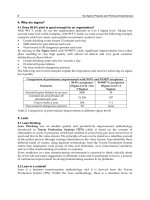
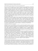
customer specification and the defects would be as minimum as possible. The table-1 below
depicts the different sigma level i.e. the Z scores and the corresponding DPMO with
remarks indicating typical industry level benchmarks.

Z
ST
DPMO Remarks
6 3.4 World-class
5 233 Significantly above average
4.2 3470 Above industry average
4 6210 Industry average
3 66800 Industry average
2 308500 Below industry average
1 691500 Not competitive
Table 1. The DPMO at various Z-values
Z-score can be a good indicator for business parameters and a consistent measurement for
performance. The advantage of such a measure is that it can be abstracted to any industry,
any discipline and any kind of operations. For e.g. on one hand it can be used to indicate
performance of an “Order booking service” and at the same time it can represent the “Image
quality” in a complex Medical imaging modality. It manifests itself well to indicate the
quality level for a process parameter as well as for a product parameter, and can scale
conveniently to represent a lower level Critical to Quality (CTQ) parameter or a higher level
CTQ. The only catch is that the scale is not linear but an exponential one i.e. a 4-sigma
process/product is not twice as better as 2-sigma process/product. In a software
development case, the Kilo Lines of code developed (KLOC) is a typical base that is taken to

represent most of the quality indicators. Although not precise and can be manipulated, for
want of better measure, each Line of code can be considered an opportunity to make a
defect. So if a project defect density value is 6 defects/KLOC, then it can be translated as
6000 DPMO and the development process quality can be said to operate at 4-sigma level.
Practical problem: “Content feedback time” is an important performance related CTQ for the
DVD Recorder product measured from the time of insertion of DVD to the start of playback.
The Upper limit for this is 15 seconds as per one study done on human irritation thresholds.
The figure-6 below shows the Minitab menu options with sample data as input along with
USL-LSL and the computed Z-score.


Fig. 6. Capability Analysis : Minitab menu options and Sample data

Six Sigma Projects and Personal Experiences

132
2.2.2 The capability index (Cp)
Capability index (Cp) is another popular indicator that is used in Six sigma projects to denote
the relation between “Voice of customer” to “Voice of process”. Voice of customer (VOC) is
what the process/product must do and Voice of process (VOP) is what the process/product
can do i.e. the spread of the process.
Cp = VOC/VOP = (USL-LSL)/6
This relation is expressed pictorially by the figure-7 below


Fig. 7. Capability Index Definition
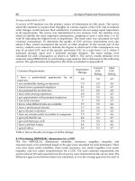
There is striking similarity between the definitions of Cp and the Z-score and for a centered
normally distributed process the Z-score is 3 times that of Cp value. The table-2 below
shows the mapping of the Z-score and Cp values with DPMO and the corresponding Yield.


Z
ST
DPMO Cp Yield
6 3.4 2 99.9997 %
5 233 1.67 99.977 %
4.2 3470 1.4 99.653 %
4 6210 1.33 99.38 %
3 66800 1 93.2 %
2 308500 0.67 69.1 %
1 691500 0.33 30.85 %
Table 2. Cp and its relation to Z-score
3. Inferential statistics
The “statistics” are valuable when the entire population is not available at our disposal and
we take a sample from population to infer about the population. These set of mechanisms
wherein we use data from a sample to conclude about the entire population are referred to
as “Inferential statistics”.
3.1 Population and samples
“Population” is the entire group of objects under study and a “Sample” is a representative
subset of the population. The various elements such as average/standard deviation

Demystifying Six Sigma Metrics in Software

133
calculated using entire population are referred to as “parameters” and those calculated from
sample are called “statistics” as depicted in figure-8 below.


Fig. 8. Population and Samples
3.2 The confidence intervals
When a population parameter is being estimated from samples, it is possible that any of the

sample A, B, C etc as shown in figure-9 below could have been chosen in the sampling
process.


Fig. 9. Sampling impact on Population parameters
If the sample-A in figure-9 above was chosen then the estimate of population mean would
be same as mean of sample-A, if sample B was chosen then it would have been the same as
sample B and so on. This means depending on the sample chosen, our estimate of
population mean would be varying and is left to chance based on the sample chosen. This is
not an acceptable proposition.
From “Central Limit theorem“ it has been found that for sufficiently large number of samples
n, the “means“ of the samples itself is normally distributed with mean at  and standard
deviation of /sqrt (n).
Hence mathematically :
nszx /




Six Sigma Projects and Personal Experiences

134
Where x is the sample mean, s is the sample standard deviation;  is the area under the
normal curve outside the confidence interval area and z-value corresponding to . This
means that instead of a single number, the population mean is likely to be in a range with
known level of confidence. Instead of assuming a statistics as absolutely accurate,
“Confidence Intervals“ can be used to provide a range within which the true process statistic
is likely to be (with known level of confidence).
 All confidence intervals use samples to estimate a population parameter, such as the
population mean, standard deviation, variance, proportion

 Typically the 95% confidence interval is used as an industry standard
 As the confidence is increased (i.e. 95% to 99%), the width of our upper and lower
confidence limits will increase because to increase certainty, a wider region needs to be
covered to be certain the population parameter lies within this region
 As we increase our sample size, the width of the confidence interval decreases based on
the square root of the sample size: Increasing the sample size is like increasing
magnification on a microscope.
Practical Problem: “Integration & Testing” is one of the Software development life cycle
phases. Adequate effort needs to be planned for this phase, so for the project manager the
95% interval on the mean of % effort for this phase from historical data serves as a sound
basis for estimating for future projects. The figure-10 below demonstrates the menu options
in Minitab and the corresponding graphical summary for “% Integration & Testing” effort.
Note that the confidence level can be configured in the tool to required value.
For the Project manager, the 95% confidence interval on the mean is of interest for planning
for the current project. For the Quality engineer of this business, the 95% interval of
standard deviation would be of interest to drill down into the data, stratify further if
necessary and analyse the causes for the variation to make the process more predictable.


Fig. 10. Confidence Intervals : Minitab menu options and Sample Data

Demystifying Six Sigma Metrics in Software

135
3.3 Hypothesis tests
From the undertsanding of Confidence Intervals, it follows that there always will be some
error possible whenever we take any statistic. This means we cannot prove or disprove
anything with 100% certainity on that statistic. We can be 99.99% certain but not 100%.
“Hypothesis tests“ is a mechanism that can help to set a level of certainity on the observations
or a specific statement. By quantifying the certainity (or uncertainity) of the data, hypothesis

testing can help to eliminate the subjectivity of the inference based on that data. In other
words, this will indicate the “confidence“ of our decision or the quantify risk of being wrong.
The utility of hypothesis testing is primarily then to infer from the sample data as to
whether there is a change in population parameter or not and if yes with what level of
confidence. Putting it differently, hypothesis testing is a mechanism of minimizing the
inherent risk of concluding that the population has changed when in reality the change may
simply be a result of random sampling. Some terms that is used in context of hypothesis
testing:
 Null Hypothesis – H
o
: This is a statement of no change
 Alternate Hypothesis - H
a
: This is the opposite of the Null Hypothesis. In other words
there is a change which is statistically significant and not due to randomness of the
sample chosen
 -risk : This is risk of finding a difference when actually there is none. Rejecting H
o
in a
favor of H
a
when in fact H
o
is true, a false positive. It is also called as Type-I error
 -risk : This is the risk of not finding a difference when indeed there is one. Not
rejecting H
o
in a favor of H
a
when in fact H

a
is true, a false negative. It is also called as
Type-II error.
The figure-11 below explains the concept of hypothesis tests. Referring to the figure-11, the
X-axis is the Reality or the Truth and Y-axis is the Decision that we take based on the data.


Fig. 11. Concept of Hypothesis Tests
If “in reality” there is no change (Ho) and the “decision” based on data also we infer that
there is no change then it is a correct decision. Correspondingly “in reality” there is a
change and we conclude also that way based on the data then again it is a correct
decision. These are the boxes that are shown in green color (top-left & bottom-right) in the
figure-11.
If “in reality” there is no change (H
o
) and our “decision” based on data is that there is
change(H
a
), then we are taking a wrong decision which is called as Type-I error. The risk of

Six Sigma Projects and Personal Experiences

136
such an event is called as

-risk and it should be as low as possible. (1-

is then the
“Confidence” that we have on the decision. The industry typical value for  risk is 5%.
If “in reality” there is change (H

a
) and our “decision” based on data is that there is no change
(H
o
), then again we are taking a wrong decision which is called a Type-II error. The risk of
such an event is called as

-risk. This means that our test is not sensitive enough to detect the
change; hence (1-

is called as “power of test”.
The right side of figure-11 depicts the old and the new population with corresponding  and
areas.
Hypothesis tests are very useful to prove/disprove the statistically significant change in the
various parameters such as mean, proportion and standard deviation. The figure-12 below
shows the various tests available in Minitab tool for testing with corresponding menu
options list.


Fig. 12. The Various Hypothesis Tests and the Minitab Menu options
3.3.1 One-sample t-test
1-sample t-test is used when comparing a sample against a target mean. In this test, the null
hypothesis is “the sample mean and the target are the same”.
Practical problem: The “File Transfer speed“ between the Hard disk and a USB (Universal
Serial Bus) device connected to it is an important Critical to Quality (CTQ) parameter for the
DVD Recorder product. The target time for a transfer of around 100 files of average 5 MB
should not exceed 183 seconds.
This is a case of 1-Sample test as we are comparing a sample data to a specified target.
Statistical problem :
Null Hypothessis H

o
: 
a
= 183 sec
Alternate Hypothesis H
a
: 
a
> 183 sec or H
a
: 
a
< 183 sec or H
a
: 
a


183 sec
Alpha risk  = 0.05
The data is collected for atleast 10 samples using appropriate measurement methods such as
stop-watch etc. The figure-13 below shows the menu options in Minitab to perform this test.
After selecting 1-sample T-test, it is important to give the “hypothesized mean” value. This is
the value that will be used for Null hypothesis. The “options” tab gives text box to input the
Alternative hypothesis. Our H
a
is H
a
: 
a

> 183 seconds. We select “greater than” because
Minitab looks at the sample data first and then the value of 183 entered in the “Test Mean”.
It is important to know how Minitab handles the information to get the “Alternative
hypothesis” correct.

Demystifying Six Sigma Metrics in Software

137

Fig. 13. 1-Sample t-test : Minitab menu options and Sample Results
 The test criteria was  = 0.05, which means we were willing to take a 5% chance of
being wrong if we rejected Ho in favor of Ha
 The Minitab results show the p-value which indicates there is only a 3.9% chance of
being wrong if we reject Ho in favor of Ha
 3.9% risk is less than 5%; therefore, we are willing to conclude Ha. The file-transfer, on
average, is taking longer than 183 seconds between USB-Hard Disk
The same test would be performed again after the improvements were done to confirm the
statistically significant improvement in the file-transfer performance is achieved.
3.3.2 Two-sample t-test
2-sample t-test can be used to check for statistical significant differences in “means” between
2 samples. One can even specify the exact difference to test against. In this test, the null
hypothesis is “there is no difference in means between the samples”.
Practical problem : The “Jpeg Recognition Time“ is another CTQ for the DVD recorder
product. The system (hardware+software) was changed to improve this perfromance. From
our perspective the reduction in average recognition time has be more than 0.5 sec to be
considered significant enough from a practical perspective.
This is a case of 2-Sample test as we are comparing two independent samples.
Statistical problem :
Null Hypothessis H
o

: 
Old

New
sec
Alternate Hypothesis H
a
: 
Old

New
sec
Alpha risk  = 0.05
The data is collected for atleast 10 samples using appropriate measurement methods for the
old and the new samples.
The figure-14 below shows the menu options in Minitab to perform this test. After selecting
2-sample T-test, either the summarized data of samples can be input or directly the sample
data itself. The “options” tab gives box to indicate the Alternative hypothesis. Based on
what we have indicated as sample-1 and sample-2, the corresponding option of “greater
than” or “less than” can be chosen. It also allows to specify the “test difference” that we are
looking for which is 0.5 seconds in this example.

Six Sigma Projects and Personal Experiences

138

Fig. 14. 2-Sample t-test : Minitab menu options and Sample Results
 The criteria for this test was  = 0.05, which means we were willing to take a 5% chance
of being wrong if we rejected H
o

in favor of H
a

 The Minitab results show the p-value which indicates there is only a 0.5% chance of
being wrong if we reject H
o
in favor of H
a

 0.5% risk is less than 5%; therefore, we are willing to conclude H
a
. The Sample-New
has indeed improved the response time by more than 0.5 seconds
 The estimate for that difference is around 0.74 seconds


The above two sections has given some examples of setting up tests for checking differences
in mean. The philosophy remains the same when testing for differences in “proportion” or
“Variation”. Only the statistic behind the check and the corresponding test changes as was
shown in the figure-12 above.
3.4 Transfer functions
An important element of design phase in a Six sigma project is to break down the CTQs (Y)
into lower level inputs (Xs) and a make a “Transfer Function”. The purpose of this transfer
function is to identify the “strength of correlation” between the “Inputs (Xs)” and output (Y) so
that we know where to focus the effort in order to optimise the CTQ. The purpose of this
exercise also is to find those inputs that have an influence on the output but cannot be
controlled. One such category of inputs is “Constants or fixed variables (C)”and other category
is “Noise parameters (N)”. Both these categories of inputs impact the output but cannot be
controlled. The only difference between the Constants and the Noise is the former has
always a certain fixed value e.g. gravity and the latter is purely random in nature e.g.

humidity on a given day etc.
There are various mechanisms to derive transfer functions such as regression analysis,
Design of experiments or as simple as physical/mathematical equations. These are
described in the below sections.
3.4.1 Physics/Geometry
Based on the domain knowledge it is possible to find out the relationship between the CTQ
(Y) and the factor influencing it (Xs). Most of the timing/distance related CTQs fall under

Demystifying Six Sigma Metrics in Software

139
this category where total time is simply an addition of its sub components. These are called
as “Loop equations”. For e.g.
Service time(Y) = Receive order(x1) +Analyse order(x2) +Process order(x3) +Collect payment (x4)
Some part of the process can happen in parallel. In such cases
Service time(Y)=Receive order(x1)+Analyse order(x2)+Max(Process order(x3), Collect payment(x3))
Practical problem :
“Recording duration” (i.e. number of hours of recording possible) is one of the CTQs for the
DVD recorder as dictated by the marketing conditions/competitor products. The size of
hard disk is one of the factors influencing the duration. Each additional space comes at a
cost hence it is important to optimise that as well. The transfer function in this case is the
one that translates available memory space (in Gigabytes) into time (hours of recording).
From domain knowledge this translation can be done using audio bit rate and video bit rate
as follows:
b = ((video_bitrate * 1024 * 1024)/8) + ((audio_bitrate*1024)/8) bytes
k = b/1024 kilobytes
no. of hrs of recording = ((space_in GB)*1024*1024)/(k*3600)
3.4.2 Regression analysis
“Regression Analysis” is a mechanism of deriving transfer function when historical data is
available for both the Y and the Xs. Based on the scatter of points, regression analysis

computes a best fit line that represents the relation of X to Y minimizing the “residual error”.
Practical Problem:
“Cost of Non-Quality (CONQ)” is a measure given to indicate the effort/cost that is spent on
rework. If it was “right” the first time this effort could have been saved and maybe utilised
for some other purpose. In a software development scenario, because there are bugs/issues
lot of effort is spent on rework. Not only it is additional effort due to not being right the first
time, but also modifying things after it is developed always poses risks due to regression
effects. Hence CONQ is a measure of efficiency of the software development process as well
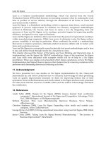
as indirect measure for first-time-right quality. Treating it as CTQ (Y), the cause-effect
diagram in figure-15 below shows the various factors (Xs) that impact this CONQ. This is
not an exhaustive list of Xs and there could be many more based on the context of the
project/business.


Fig. 15. Factors Impacting CONQ

Six Sigma Projects and Personal Experiences

140
Since lot of historical data of past projects is available, regression analysis would be a good
mechanism to derive the transfer function with Continuous Y and Continuous Xs. Finding
the relation between Y and multiple Xs is called “Multiple Regression” and that with single X
is referred to as “Simple Regression”. It would be too complicated to do the analysis with all
Xs at the same time; hence it was decided to choose one of the Xs in the list that has a higher
impact, which can be directly controlled and most importantly which is “continuous” data
for e.g. Review effort. The figure-16 below shows the Regression model for CONQ.


Fig. 16. The Regression Analysis for CONQ
When concluding the regression equation, there are 4 things that need to be considered:-

1. The p-value. The Null hypothesis is that “there is no correlation between Y and X”. So if p-
value < then we can safely reject Null and accept the Alternate, which is that Y and X
are correlated. In this case p-value is 0, this means that we can conclude that the
regression equation is statistically significant
2. Once the p-value test is passed, the next value to look at is R
2
(adj). This signifies that the
amount of variability of Y that is explained by the regression equation. Higher the R
2

better it is. Typical values are > 70%. In this case, R
2
(adj) value is 40%. This indicates
that only 40% of variability in CONQ is explained by the above regression equation.
This may not be sufficient but in R&D kind of situation especially in software, where
the number of variables are high, R
2
(adj) value of 40% and above could be considered a
reasonable starting point
3. The third thing is then to look at the residuals. A Residual is the error between the fitted
line (regression equation) and the individual data points. For the regression line to be
un-biased, the residuals themselves must be normally distributed (random). A visual
inspection of the residual plots as shown in figure-17 below can confirm that e.g. a
lognormal plot of residuals should follow a straight line on the “normal probability
plot” and residuals should be either side of 0 in the “versus fits” plot. The “histogram”
in the residual plot can also be good indication.
4. Once the above 3 tests pass, the regression equation can be considered statistically
significant to predict the relations of X to Y. However one important point to note is the
“range of values for X” under which this equation is applicable. For e.g. the above CONQ
equation can be used only in the range of Review % from 0 to 6% as the regression

analysis was done with that range.