A Complete Control Scheme for Variable Speed Stall Regulated Wind Turbines
319
The same mechanism holds for the propagation of the covariance 

of the true state 
around its mean .
As can be seen from Eqns. 12-16 the Kalman filter in principle contains a copy of the applied
dynamic system, the state vector of which, 

is corrected at every update step by the
correcting term 




|
 of Eqn. 14. The expression inside the parenthesis is
called the Innovation sequence of the Kalman filter:






|

(17)
which is equal to the estimation error at every time step. When the Kalman filter state
estimate is optimum, 


is a white noise sequence (Chui & Chen, 1999). The operation of any
Q and R adaptation algorithms that are included in the Kalman filter is based on the
statistics of the innovation sequence (Bourlis & Bleijs, 2010a, 2010b).
Regarding the stability of the Kalman filter algorithm, this is always guaranteed providing
that the dynamic system of Eqns. 8-9 is stable and that Q and R have been selected
appropriately. In the case of the wind turbine, the dynamic system is always stable, since in
Eqns. 8-9 only the dynamics of the drivetrain are included, which have to be stable by
default. In addition, the Q and R are continuously updated appropriately by adaptive
algorithms and the stability of the adaptive Kalman filter can be easily assessed through
software or hardware simulations.
From the above it becomes obvious that the stability of the closed loop control system of
Figs. 6-7 is then guaranteed provided that the speed controller stabilizes the system.
5.2 Adaptive Kalman filtering and advantages
In order to see the advantage of the adaptive Kalman filter over the simple Kalman filter,
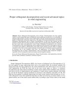
software simulations of aerodynamic torque estimation for a 3MW wind turbine for
different wind conditions are shown in Figs. 8 (a-b).
From the below figures the advantage of the adaptive Kalman filter compared to the
nonadaptive one can be observed. Specifically, the torque estimate obtained by the adaptive
filter achieved similar time delay in high wind speed, but much improved performance in
low wind speeds.
The adaptive Kalman filter can be realized by incorporating Q and/or R adaptation routines
in the Kalman filter algorithm, as mentioned in (Bourlis & Bleijs, 2010a, 2010b).



0 0.5 1 1.5 2 2.5 3 3.5
x 10
4
0
1

2
3
4
5
6
7
x 10
6
Time (*0.005 sec)
Ta (Nm)
Actual and estimated Ta
(a)



Actual and estimated aerodynamic torque


Fundamental and Advanced Topics in Wind Power
320









Fig. 8. T

a
(blue) and 


(red) of a 3MW wind turbine: (a) For high wind speeds with a
Kalman filter, (b) for high wind speeds with an adaptive Kalman filter, (c) for low wind
speeds with a Kalman filter and (d) for low wind speeds with an adaptive Kalman filter.
6. Speed reference determination
As mentioned earlier, an estimate of the effective wind speed 

is used for the determination
of the generator speed reference. This can be extracted by numerically solving Eqn. 3 using
the Newton-Raphson method.
0 0.5 1 1.5 2 2.5 3 3.5
x 10
4
0
1
2
3
4
5
6
7
x 10
6
Time (*0.005 sec)
Ta (Nm)
Actual


and

estimated

Ta
0 0.5 1 1.5 2 2.5 3 3.5
x 10
4
0
2
4
6
8
10
x 10
5
Time (*0.005 sec)
Ta (Nm)
Actual and estimated Ta
0 0.5 1 1.5 2 2.5 3 3.5
x10
4
0
1
2
3
4
5
6
7

8
9
10
x 10
5
Time
(
*0.005 sec
)
T
a
(N
m
)
Actual and estimated Ta
(b)
(d)
(c)


Time (*0.005 sec)

Time (*0.005 sec)






Actual and estimated aerodynamic torque



Actual and estimated aerodynamic torque
Actual and estimated aerodynamic torque
Time (*0.005 sec)


A Complete Control Scheme for Variable Speed Stall Regulated Wind Turbines
321
In order for the Newton-Raphson method to be applied, the C
p
-λ characteristic of the rotor is
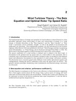
analytically expressed using a polynomial. Fig. 9 shows the C
p
curve of a Windharvester
wind turbine rotor and its approximation by a 5
th
order polynomial.


Fig. 9. Actual C
p
curve (red) and approximation using a 5
th
order polynomial (blue).
Fig. 10 shows T
a
versus V for a fixed value of ω, for a stall regulated wind turbine. As can be
seen, T
a

after exhibiting a peak, drops and then starts rising again towards higher wind
speeds (Biachi et al., 2007). Fig. 10 also displays three possible V solutions V
1
, V
2
and V
3
corresponding to an arbitrary aerodynamic torque level T
a
=T
aM
, given the fixed ω.


Fig. 10. T
a
versus V for fixed ω.
Also, Fig. 11 shows a graph similar to that of Fig. 10 for ω=ω
N
, where 


and 

/

are the
aerodynamic torque levels corresponding to the points B and C of Fig. 5 respectively.



Fig. 11. T
a
versus V for ω=

.
1 2 3 4 5 6
0
0.05
0.1
0.15
0.2
0.25
0.3
0.35
0.4
0.45
0.5
tip-speed ratio
Cp
Cp curve and approximation

Fundamental and Advanced Topics in Wind Power
322
For the part AB of Fig. 5, the optimum speed reference is: 








, where V
1
is the lowest
V solution seen in Fig. 10. Also, for the part BC the speed reference is: 



. In
addition, from Fig. 11 it can be seen that for ω=

when V
1
>


, the aerodynamic torque is
always T
a
>


, so there is a monotonic relation between V
1
and T
a
. Therefore, V
1
can be
effectively used in order to switch between the parts AB and BC. So, 


for the part ABC
can be expressed as:








,






,




,
(18)
Regarding V
1
, it

can be easily obtained with a Newton-Raphson if this is initialized at an

appropriate point, as seen in Fig. 12, where the expression 




versus V is shown.


Fig. 12. Newton-Raphson routine NR
1
used for V solution extraction of Eqn. 3.
Fig. 13 shows the actual V and its estimate, 

obtained in Simulink using the Newton-
Raphson routine for the model of the aforementioned Windharvester wind turbine.


Fig. 13. Actual V (blue) and estimated 

(red) using NR
1
.
As can be seen, the wind speed estimation is very accurate. In the next section, the speed
control design is described.
7. Gain scheduled proportional-integral speed controller
The speed controller should satisfy conflicting requirements, such as accurate speed
reference tracking and effective disturbance rejection due to high frequency components of
0.5 1 1.5 2 2.5 3 3.5
x 10
4

3
4
5
6
7
8
9
Time (*0.005 sec)
V ( m/sec)
Actual and estimated V without dynamic inflow effects simulated
Actual and estimated effective wind s
p
eed



A Complete Control Scheme for Variable Speed Stall Regulated Wind Turbines
323
the aerodynamic torque, but at the same time should not induce high cyclical torque loads
to the drivetrain, via excessive control action. In addition, the controller should limit the
torque of the generator to its rated torque, T
N
and also not impose motoring torque.
Although all the above objectives can be satisfied by a single PI controller, as shown in
(Bourlis & Bleijs, 2010a), this cannot be the case in general, due to the highly nonlinear
behavior of the wind turbine, due to the rotor aerodynamics. Specifically, the nonlinear
dependence of T
a
to ω through Eqn. 3, establishes a nonlinear feedback from ω to T
a

and due
to this feedback, the wind turbine is not unconditionally stable. The dynamics are stable for
below rated operation, close to the C
pmax
, where the slope of the C
q
curve is negative (see Fig.
3) and therefore causes a negative feedback, but unstable for stall operation (operation on
the left hand side of the C
q
curve, where its slope is positive), (Biachi et al., 2007; Novak et
al., 1995).
A single PI controller may marginally satisfy stability and performance requirements, but in
general it cannot be used when high control performance is required. High performance
requires very effective maximum power point tracking and at the same time very effective
power regulation for above rated conditions and for Mega Watt scale wind turbines, which
are now under demand, trading off between these two objectives is not acceptable, due to
economic reasons.
Specifically, for below rated operation and until ω
Ν
is reached, the speed reference for the
controller follows the wind variations. For this operating region moderate values of the
control bandwidth are required for acceptable reference tracking. Although tracking of
higher frequency components of the wind would increase the energy yield, it would
simultaneously increase the torque demand variations, which would induce higher cyclical
loads to the drivetrain.
For constant speed operation (part BC in Fig. 5) the requirements are a bit different. At this
region, the wind acts as a disturbance that tries to alter the fixed rotational speed of the
wind turbine. Considering that at this region the aerodynamic torque increases
considerably, before it reaches its peak (see Fig. 11), where stall starts occurring, the

controller should be able to withstand to potential rotational speed increases, as this could
lead to catastrophic wind up of the rotor. For this reason, at this operating region a higher
control bandwidth is required.
Further, in the stall region, it is known from (Biachi et al., 2007) that the wind turbine has
unstable dynamics, with Right Half Plane zeros and poles. Therefore, different bandwidth
requirements exist for this region too.
A type of speed controller that can effectively overcome the above challenges, while at the
same time is easy to implement and tune in actual systems, is the gain scheduled PI
controller. This type of controller consists of several PI controllers, each one tuned for a
particular part of the operating region. Depending on the operating conditions, the
appropriate controller is selected each time by the system, satisfying that way the local
performance requirements.
In order to avoid bumps of the torque demand that can occur during the switching from one
controller to another, the controller is equipped with a bumpless transfer controller, which
guarantees a smooth transition between them. The bumpless transfer controller in principle
ensures that all the neighbouring controllers have exactly the same output with the active
one, so no transient will happen during the transition. For this reason for every PI controller
there is a bumpless transfer controller, which measures the difference of its output with the
active one and drives it appropriately through its input. Fig. 14 shows a schematic of a gain
scheduled controller consisting of two PI controllers.

Fundamental and Advanced Topics in Wind Power
324


Fig. 14. Gain scheduled controller with bumpless transfer circuit.
As can be seen in Fig. 14, there is a Switch Command (SC) signal that selects the control
output via switch “s2”. The same signal is responsible for the activation of the bumpless
transfer controller. Specifically, when “controller 2” is activated, the bumpless transfer
controller for “controller 1” is activated too. The bumpless transfer controller receives as

input the difference of the outputs of the two controllers and drives “controller 1” through
one of its inputs such that this difference becomes zero. It is mentioned the same bumpless
transfer controller exists for “controller 2”, but if the dynamic characteristics of the two
controllers are not very different, a single bumpless transfer controller can be used for both
of them, when only two of them are used.
Regarding the PI controllers used, they have the proportional term applied only to the
feedback signal, (known as I-P controller (Johnson & Moradi, 2005; Wilkie et al, 2002)). The
I-P controller exhibits a reduced proportional kick and smoother control action under
abrupt changes of the reference. The structure of this controller is shown in Fig. 15(a). In Fig.
15(b) the discrete time implementation of the controller with Matlab/Simulink blocks is
shown. The implementation also includes a saturation block, which limits the output torque
demand to the specified levels (generating demands up to T
N
) and an anti-windup circuit,
which stops the integrating action during saturation.



Fig. 15. (a) I-P controller diagram (Johnson & Moradi, 2005) and (b) Simulink
implementation.
In the following section, a case design study for the Windharvester wind turbine is
presented.
(a)
(b)

A Complete Control Scheme for Variable Speed Stall Regulated Wind Turbines
325
8. Case design study
The analysis that follows is based on data from a 25kW Windharvester constant speed stall
regulated wind turbine that has been installed at the Rutherford Appleton Laboratory in

Oxfordshire of England. The control system that has been described in the previous sections
has been designed for this wind turbine and the complete system has been simulated in a
hardware-in-loop wind turbine simulator.
8.1 Description and parameters of the Windharvester wind turbine
This wind turbine has a 3-bladed rotor and its drivetrain consists of a low speed shaft, a
step-up gearbox and a high speed shaft. In fact, the gear arrangement consists of a fixed-
ratio gearbox, followed by a belt drive. This was originally intended to accommodate
different rotor speeds during the low wind and high wind seasons. The drivetrain can be
seen in Fig. 16, where the belt drive is obvious. The generator is a 4-pole induction
generator.


Fig. 16. Drivetrain of the Windharvester wind turbine.
The data for this wind turbine are given in Table 1.

Rotor inertia, I
1
14145 Kgm
2

Gearbox inertia, I
g

34.2 Kgm
2

Generator inertia, I
2
0.3897 Kgm
2


LSS stiffness, K
1
3.36•10
6
Nm/rad
HSS stifness, K
2
2.13•10
3
Nm/rad
Rotor radius, R 8.45 m
Gearbox ratio, N 1:39.16
LSS rated rotational frequency, ω
1
4.01 rad/sec
Table 1. Wind turbine data.

Fundamental and Advanced Topics in Wind Power
326
The C
p
and C
q
curves of the rotor of the wind turbines are shown in Fig. 17 (a) and (b)
respectively (in blue). In addition, the data have been slightly modified in order to obtain
the steeper C
p
and C
q

curves, shown in red colour. As mentioned before, the steeper C
p

curve requires less speed reduction during stall regulation at constant power and therefore
it can be preferred for a variable speed stall regulated wind turbine. However, such a C
p

curve requires more accurate control in below rated operation. Thus, the modified curves
are also used to assess the performance of the proposed control methods for below rated
operation.
The maximum power coefficient C
pmax
=0.45 is obtained for a tip speed ratio λ
Cpmax
=5.02,
while the maximum torque coefficient is C
qmax
=0.098 for a tip speed ratio λ
Cqmax
=4.37.


Fig. 17.

(a) Power and (b) torque coefficient curve of the rotor of the Windharvester wind
turbine.
8.2 Dynamic analysis of the wind turbine

The dynamics of the wind turbine are mainly represented by Eqns. 19-23 after the drivetrain
has been modeled as a system with three masses and two stifnesses as shown in Fig. 18.







1
2






,










(19)

















(20)














(21)









(22)








(23)
As can be seen, the dynamic model of Eqns. 19-23 is nonlinear with two inputs V and T
g

(generator torque). Output of the model is the generator speed 

, which is the only speed
measurement available in commercial wind turbines. In order for the model to be analyzed,
the term 

of Eqn. 19, shown in Fig. 17(b), is approximated with a polynomial and the
whole model is linearized (Biachi et al., 2007). Then, the transfer functions from its inputs to

(a) (b)


A Complete Control Scheme for Variable Speed Stall Regulated Wind Turbines
327

Fig. 18. Wind turbine drivetrain: (a) schematic, (b) dynamic model.


Fig. 19. Bode plots of 


for below rated (blue) and above rated (stall) operation (red).


Fig. 20. Bode plots of 




for below rated (blue) and above rated (stall) operation (red).
-250
-200
-150
-100
-50
0
50
Magni tude (dB
)
10
-3
10

-2
10
-1
10
0
10
1
10
2
10
3
10
4
-450
-360
-270
-180
-90
0
Phase ( deg)
Bode Diagram
Fre
q
uenc
y

(
rad/sec
)
-150

-100
-50
0
50
Magnitude (dB)
10
-3
10
-2
10
-1
10
0
10
1
10
2
10
3
-720
-540
-360
-180
0
180
Phase (deg)
Bode Diagram
Frequency (rad/sec)

Fundamental and Advanced Topics in Wind Power

328
its output, 


and 




are examined for different operating conditions. The Bode plots of



and 




are shown in Figs. 19 and 20 respectively, for two operating points, namely
one for below rated operation (ω
1
,V)=(4rad/sec, 6.76m/sec) and one for above rated
operation, (4 rad/sec, 8.76m/sec).
As can be seen from the above plots, a phase change of 180
°
occurs, for frequencies less than
0.1rad/sec as the operating point of the wind turbine moves from below rated to stall
operation, for both transfer functions. In addition, the first drivetrain mode can be observed
at 53rad/sec.
8.3 Control design


In this section the design of the speed controller for the Windharvester wind turbine is
presented. In Fig. 21 the actual T
a
-ω plot for the simulated wind turbine including the
operating point locus (black), is shown. In the plot T
a
-ω characteristics are shown in blue
colour and the characteristics for wind speeds above 20m/sec are shown with bold line. The
brown curve corresponds to operation for 


6.76m/sec where operation at constant
speed ω=ω
Ν
starts. The green curve corresponds to V
N
=8.3m/sec, where P
N
=25kW. Also the
hyperbolic curve of constant power P
N
=25kW is shown in red.


Fig. 21. Actual T
a
-ω plot of the simulated wind turbine.
The operating point locus is shown in black and starts at ω
Α

=2.1rad/sec for V
cut-in
=3.5m/sec.
Regarding the gain scheduled controller, two PI controllers are used, with PI gains of 20 and
10 Nm/rad/sec for operation below ω
Ν
and 30 and 50Nm/rad/sec for operation above ω
Ν
.
Fig. 22 shows the Bode plots of the closed loop transfer function from the reference
rotational speed ω
ref
(see Fig. 7) to the generator speed ω
2
, 




for the two controllers
used. Fig. 23 shows the corresponding Bode plots for the disturbance transfer function from
the wind speed V to ω
2
, 


. These Bode plots have been obtained for operating conditions
(V,ω)=(6.76m/sec, 4rad/sec).

A Complete Control Scheme for Variable Speed Stall Regulated Wind Turbines

329

Fig. 22. Bode plots of 




for ω
1
=4rad/sec and V=6.76m/sec. Controller for operation
below (blue) and above (red) ω
Ν
.

Fig. 23. Bode plots of 


for ω
1
=4rad/sec and V=6.76m/sec for the above controllers.
As can be seen from Fig. 22, the first controller achieves a closed loop speed control bandwidth
of 0.6rad/sec and the second 3rad/sec. Through hardware simulations these values were
considered sufficient as will be seen later. From Fig. 23 it can be also seen that the first
controller achieves good disturbance rejection for frequencies below 0.2rad/sec, which is
absolutely satisfactory, since disturbance rejection extended to higher frequencies increases the
torque demand variations, which would not be desirable. Fig. 23 shows that the disturbance
rejection of the second controller is very improved, which is the main requirement for this
operating region, as this was mentioned in the previous section. Finally, from the graphs it can
be observed that both controllers effectively suppress the first drivetrain mode at 53rad/sec,
achieving a gain of -40 and -28dBs at this frequency, respectively (Fig. 22).

-200
-150
-100
-50
0
50
Magnitude ( dB)
10
-2
10
-1
10
0
10
1
10
2
10
3
10
4
-270
-180
-90
0
Phase (deg)
Bode Diagram
Frequency (rad/sec)
-250
-200

-150
-100
-50
0
50
Magnit ude (dB)
10
-2
10
-1
10
0
10
1
10
2
10
3
10
4
-540
-360
-180
0
180
Phase (deg)
Bode Diagram
Frequency (rad/sec)

Fundamental and Advanced Topics in Wind Power

330
8.4 Hardware-in-loop simulator
In this section the hardware-in-loop simulator developed in the laboratory for the testing of
the proposed control system is briefly described. The simulator was developed such that the
dynamics of the Windharvester and in general of every wind turbine are represented with
high accuracy. It consists of a dSPACE ds1103 simulation platform and two cage Induction
Machines (IM) rated at 3kW connected back-to-back via a stiff coupling. One of them acts as
the prime mover and the other as the generator (IG). The machines are controlled by vector
controlled variable speed industrial drives.
Fig. 24 shows a diagram of the arrangement of the hardware-in-loop simulator, where it can
be seen that the proposed control system together with the dynamic model of the wind
turbine (WT) (Eqns. 19-23) run in real time via a dSPACE ds1103 board, while the 25kW
induction generator of the wind turbine is simulated by the IG. The sampling frequency
used in dSPACE is 200Hz. As can be observed there are two feedback loops, one through
T
IG
, WT model, T
D
and the IM and IG and their drives and one through the IG drive, ω
2
, the
wind turbine control system and Τ. Τhe first is used for the simulation of the wind turbine,
while the second simulates the control system of the wind turbine. As can be seen, the
control system commands the IG drive with torque signal T. The wind turbine model is
driven by wind speed timeseries, which have been obtained by the Rutherford Appleton
Laboratory.


Fig. 24. Hardware-in-loop simulator.
Fig. 25 shows an ensemble of the effective wind speed V, simulated in the hardware-in-loop

simulator. The effective wind speed has also been enhanced with considerable amount of
energy at higher harmonics, in order to test the effectiveness of the control system in
extreme conditions. The corresponding spectrum is shown in Fig.26 (blue), where it is
compared with the spectrum of the harmonic free wind series obtained by the Rutherford
Appleton Laboratory (green).
8.5. Hardware simulation results
Here simulation results of the proposed control system using the hardware-in-loop
simulator for below rated operation are presented. The simulations results shown have been
obtained using the steeper C
p
-λ characteristic of Fig. 17 and the results in terms of energy
yield in maximum power point operation are compared with the ones achieved with the
conventional control law of Eqn. 6 (Eqn. 7 gives similar performance). It is mentioned that
the applied wind series has been scaled down to the specified levels (below V
N
=8.3m/sec).


A Complete Control Scheme for Variable Speed Stall Regulated Wind Turbines
331


Fig. 25. Effective wind speed V.

Fig. 26. Spectrum of V (blue) and of the original wind series (green).

Figs. 27-32 show simulation results using the steep C
p
-λ characteristic. For these simulation
results, maximum power point operation has been extended up to 7.5m/sec (so

ω
N
=4.43rad/sec), so the input wind speed has been limited at this value.


Fig. 27. Actual (blue) and estimated (red) V.
0 0.5 1 1.5 2 2.5 3 3.5
x 10
4
5
10
15
20
Time (*0.005 sec)
V ( m/sec)
Wind speed
0 1 2 3 4 5 6 7 8 9 10
-60
-50
-40
-30
-20
-10
0
10
20
Frequency (Hz)
Power Spectral Density
0 50 100 150
2

3
4
5
6
7
8
9
t (sec)
V (m/sec)
Actual and estimated effective wind speed

Effective wind speed




Fundamental and Advanced Topics in Wind Power
332

Fig. 28. Ideal (blue), estimated (red) and low pass filtered estimated generator speed
reference (black).



Fig. 29. Reference (LPF) (black) and actual (green) generator speed.


Fig. 30. Torque demand (



) (black) and actual generator torque (T
g
) (green).
0 50 100 150
40
60
80
100
120
140
160
180
t (sec)
wmega (rad/sec
)
Ideal and estimated IG speed reference
0 50 100 15
90
100
110
120
130
140
150
160
170
180
t (sec)
wmega (rad/sec)
Reference and actual IG speed

0 50 100 150
-50
0
50
100
150
200
250
t (sec)
T (Nm)
Reference and actual IG torque







Torque demand and actual generator

A Complete Control Scheme for Variable Speed Stall Regulated Wind Turbines
333

Fig. 31. Power coefficient in time.


Fig. 32. Cumulative energy with the conventional control (Eqn. 6), (black) and with the
proposed control, (green).
As can be seen from Fig. 27, the wind speed estimation is very accurate and the resulting
speed reference is quite close to the ideal one (Fig. 28). The speed reference for the generator

is low-pass filtered before it is used by the speed controller, in order to smooth out high
frequency variations. Furthermore, from Figs. 29-30 it can be seen that the speed of the
generator (N*ω) closely follows its reference and this is achieved without excessive control
action. Fig. 31 shows very effective maximum power point operation (close to C
p max
=0.45).
Finally, Fig. 32 shows a remarkable gain of 6.5% in the cumulative produced energy using
the proposed control method, compared to the conventional control method. This is a very
important result, which shows that it is possible to very effectively control a variable speed
stall regulated wind turbine for maximum power point operation, using the proposed
method.
Furthermore, the performance of the control system has been tested at constant speed
operation, at ω=ω
Ν
=4rad/sec, using the original scale of the wind speed series of Fig. 25. At
this operating region, the PI speed controller with higher gains is switched on (see Section
8.2). The performance of this controller in terms of speed reference tracking is compared
with the performance that is achieved when only the controller of lower gains is used,
according to (Bourlis & Bleijs, 2010a). Fig. 33 shows these results, while Fig. 34 shows the
control torque and the IG torque using the PI controller with higher gains, when the original
C
p
-λ curve is used.
0 50 100 150
0.2
0.25
0.3
0.35
0.4
0.45

0.5
t (sec)
Cp
Power coefficient
0 50 100 150
0
2
4
6
8
10
12
14
16
18
x 10
5
t (sec)
E (Joule)
Cumulative energy




Fundamental and Advanced Topics in Wind Power
334


Fig. 33. Reference speed (black), generator speed response with (a) PI controller with low
gains (red) and (b) with dedicated PI controller with higher gains (blue).



Fig. 34. Torque demand (


) (black) and actual (blue) IG torque for the controller with
higher gains.
As can be observed, the speed reference tracking is considerably improved using a
controller with higher gains. Specifically, the generator speed very rarely diverges further
than 2% of its reference, while with the controller with the lower gains, the speed error very
often reaches 3.1% and higher. Furthermore, from Fig. 34 it can be seen that the control
torque variations are limited to less than 40% around its average value (180Nm), which is
absolutely acceptable. This performance can be even better when the steep C
p
-λ curve is
used.
Using the proposed control method, very accurate reference tracking can be achieved
during stall regulation at constant power too. Fig. 35 shows power regulation at 25 and
20kW at above rated wind speeds, when the steeper C
p
-λ curve is simulated and using a PI
controller with PI gains of 30 and 30 Nm/rad/sec, respectively. Fig. 36 shows the generator
torque during this experiment.
As can be seen, Figs. 35 and 36 exhibit very effective power control. This is a result of
accurate speed reference tracking and very smooth control action by the control system
(examination of the speed reference determination algorithm for stall regulation is outside
of the scope of this paper).
0 20 40 60 80 100 120 140 16
0
50

100
150
200
250
300
350
t (sec)
T (Nm)
Reference and actual IG torque
(c)



Torque demand and actual generator

A Complete Control Scheme for Variable Speed Stall Regulated Wind Turbines
335

Fig. 35. Reference (black) and actual (blue) induction generator power.


Fig. 36. IG torque.
9. Conclusions
In this paper a control scheme for variable speed stall regulated wind turbines was
presented. The control system aims to continuously provide the optimum rotational speed
for the wind turbine in order to achieve maximum power production until the rated
rotational speed is reached and effective power limitation when the wind turbine operates at
wind speeds higher than the rated. The proposed control system consists of an aerodynamic
torque estimation stage, a speed reference determination stage and a gain scheduled
proportional-integral speed controller. The first two stages are used to produce the optimum

speed reference for the speed controller. The speed controller is responsible for the system to
closely follow the speed reference and at the same time for the torque loading of the
drivetrain as well as the effect of external disturbances to be kept up to specified levels.
In this paper emphasis is put on the examination of the performance of the control system in
below rated operation, while the ability of the proposed gain scheduled speed controller to
effectively achieve power limitation for above rated wind speeds is also exhibited.
The whole control scheme has been implemented in a high performance hardware-in-loop
simulator, which is driven by real wind site data. The hardware-in-loop simulator has been
developed using industrial machines and drives and is controlled by an accurate dynamic
model of an actual wind turbine, such that it closely approximates the dynamics of the wind
turbine.
0 20 40 60 80 100 120 140 160 180
1
1.5
2
2.5
3
3.5
4
x 10
4
t (sec)
P (W)
IG power with stall regulation
0 20 40 60 80 100 120 140 160 180
80
100
120
140
160

180
200
220
240
t (sec)
T (Nm)
IG torque





Fundamental and Advanced Topics in Wind Power
336
The hardware simulation results exhibited a very good performance of the proposed control
scheme in below rated operation. Specifically, the aerodynamic torque and effective wind
speed were accurately estimated, which in turn resulted in very accurate speed reference
extraction by the control system. Furthermore, the proposed gain scheduled speed controller
very effectively satisfied different bandwidth requirements for different operating regions
and at the same time provided adequate damping to the drivetrain oscillation modes and
eliminated the effects of external disturbances.
Through simulations using a steep power coefficient curve for the wind turbine rotor, which
is a requirement for a variable speed stall regulated wind turbine, the control system
achieved accurate reference tracking, which resulted in effective maximum power point
operation, as this was observed by the high values of the power coefficient achieved during
the operation. As a result, the produced cumulative energy for maximum power point
operation using the proposed control system was increased by 6.5%, when compared with
the one achieved using conventional control methods that are used in commercial wind
turbines. It is also notable that this performance was achieved without excessive control
torque action by the generator and this is possible to be achieved in general by appropriately

adjusting the bandwidth of the PI controller used, as well as the bandwidth of the low-pass
filter at the speed reference.
Furthermore, the hardware simulation results for operation at constant speed for above
rated wind speeds exhibited a very good performance of the proposed gain scheduled PI
speed controller when compared with previous implementations using a single PI controller
for the whole operating region. The proposed controller can be effectively used for speed
control during stall regulation at constant power, as this was also shown through hardware
simulations. So, this type of controller provides a suitable solution for high performance
control of stall regulated wind turbines. In addition, this controller is easy to implement and
its tuning only requires basic knowledge of control systems so it can be performed by any
experienced engineers.
A key feature of the proposed control scheme is that it can run on commercial digital signal
processor boards. From there it can communicate with the drive of the generator of the wind
turbine and the whole scheme requires only a speed measurement of the generator, which is
always available in commercial wind turbines. Also, in general for the operation of the
proposed control scheme there are no considerable requirements for computing power (a
sample time of 5msec was used here).
The proposed control scheme provides a novel and easy to implement solution, which as
was shown from the hardware simulation results provided, it can be effectively applied for
high performance control of variable speed stall regulated wind turbines, outperforming
conventional control methods, which is something that is presented for the first time.
To sum up, the control scheme for variable speed stall regulated wind turbines that is
proposed here and the simulation results that are presented are very important, because
they show that it is possible to effectively control this type of wind turbine using existing
technology. That way, the proposed control scheme gives confidence for the development of
variable speed stall regulated wind turbines in the near future and this is very important
due to the economic advantages that these wind turbines can have.
For the above reasons, future work should be directed on developing this control system in
an actual wind turbine. Challenges that have to overcome then are the uncertainty in the
knowledge of the exact parameters of the actual wind turbine as well as stochastic changes


A Complete Control Scheme for Variable Speed Stall Regulated Wind Turbines
337
of the dynamics of the wind turbine, due to the aerodynamic phenomena. The effects of
these uncertainties in the operation of the control system and in particular in the wind speed
estimation as well as in the performance of the speed controller need therefore to be
examined experimentally. That way the robustness of the proposed control system to this
kind of uncertainties can be increased appropriately, if required. Therefore, industrial
funded research can further contribute to the development of variable speed stall regulated
wind turbines.
10. Acknowledgment
I would like to thank Dr. J.A.M. Bleijs from the Electrical Power and Power Electronics
Group of the University of Leicester for his help and the Engineering and Physical Sciences
Research Council of United Kingdom for providing the funding for this study.
11. References
Anderson B.D.O. & Moore J.B. (1979). Optimal Filtering, Prentice - Hall Information and
System Sciences Series, Englewood Cliffs, N.J.
Biachi, F. D., et al. (2007). Wind Turbine Control Systems. Principles Modelling and Gain
Scheduling Design (1
st
ed.), Springer, ISBN 9871846284922, London UK
Bossanyi, E. A. (2003). The Design Of Closed Loop Controllers For Wind Turbines. Wind
Energy, Vol. 3, No. 3, pp. (149-163)
Bossanyi E.A. (2003). Wind Turbine Control for Load Reduction. Wind Energy, Vol. 6, No. 3,
(3 Jun 2003), pp. (229-244)
Boukhezzar B. & Siguerdidjane H. (2005). Nonlinear control of variable speed wind turbines
without wind speed measurement, Proceedings of the 44
th
IEEE Conference on
Decision and Control, and the European Control Conference, Seville, Spain, (December

12-15, 2005), pp. (3456-3461)
Bourlis D. & Bleijs J.A.M. (2010a). Control of stall regulated variable speed wind turbine
based on wind speed estimation using an adaptive Kalman filter, Proceedings of the
European Wind Energy Conference, Warsaw, Poland, (20-23 April 2010), pp. (242-246)
Bourlis D. & Bleijs J.A.M. (2010b). A wind estimation method using adaptive Kalman
filtering for a variable speed stall regulated wind turbine, Proceedings of the 11
th

IEEE International Conference on Probabilistic Methods Applied to Power Systems,
Singapore, (14-17 July 2010), pp. (89-94)
Chui C.K. & Chen G. (1999). Kalman filtering. With real time applications (3
rd
ed.) Springer
Connor B. & Leithead W.E. (1994). Control strategies for variable speed stall regulated wind
turbines, Proceedings of the 5
th
European Wind Energy Association Conference and
Exhibition, Thessaloniki, Greece, (10-14 Oct 1994), Vol. 1, pp. (420-424)
Goodfellow D., Smith G.A. & Gardner G. (1988). Control strategies for variable-speed wind
energy recovery, Proceedings of the BWECS Conference
Johnson M.A. & Moradi M.H. (2005). PID Control. New Identification and Design Methods,
Springer Kurtulmus F., Vardar A. & Izli N. (2007). Aerodynamic Analyses of
Different Wind Blade Profiles. Journal of Applied Sciences, pp. (663-670)
Leithead, W. E. (1990). Dependence of performance of variable speed wind turbines on the
turbulence, dynamics and control, IEE Proceedings, Vol. 137, No. 6, (November
1990)

Fundamental and Advanced Topics in Wind Power
338
Leithead W.E. & Connor B. (2000). Control of Variable Speed Wind Turbines: Design Task.

International Journal of Control, Vol. 73, No. 13, pp. (1189-1212)
Manwell, J. (2002). Wind energy explained: theory, design and application, Willey
Mercer A.S. & Bossanyi E.A. (1996). Stall regulation of variable speed HAWTS, Proceedings of
the European Wind Energy Conference, Göteborg, Sweden, (20-24 May 1996), pp.
(825-828)
Novak P., et al. (1995). Modelling and Control of Variable-Speed Wind-Turbine Drive-
System Dynamics. IEEE Control Systems Magazine, Vol. 15, No. 4, (Aug 1995), pp.
(28-38)
Østergaard, K.Z., et al. (2007). Estimation of Effective Wind Speed. Journal of Physics:
Conference Series, Vol. 75, No. 1, pp. (1-9)
Parker D.A. (2000). The design and development of a fully dynamic simulator for renewable
energy converters, Phd Thesis, University of Leicester
Wilkie J., et al. (2002). Control Engineering. An introductory course, Palgrave
15
MPPT Control Methods in Wind
Energy Conversion Systems
Jogendra Singh Thongam
1
and Mohand Ouhrouche
2

1
Department of Renewable Energy Systems, STAS Inc.
2
Electric Machines Identification and Control Laboratory, Department of Applied Sciences,
University of Quebec at Chicoutimi
Quebec
Canada
1. Introduction
Wind energy conversion systems have been attracting wide attention as a renewable energy

source due to depleting fossil fuel reserves and environmental concerns as a direct
consequence of using fossil fuel and nuclear energy sources. Wind energy, even though
abundant, varies continually as wind speed changes throughout the day. The amount of
power output from a wind energy conversion system (WECS) depends upon the accuracy
with which the peak power points are tracked by the maximum power point tracking
(MPPT) controller of the WECS control system irrespective of the type of generator used.
This study provides a review of past and present MPPT controllers used for extracting
maximum power from the WECS using permanent magnet synchronous generators
(PMSG), squirrel cage induction generators (SCIG) and doubly fed induction generator
(DFIG). These controllers can be classified into three main control methods, namely tip
speed ratio (TSR) control, power signal feedback (PSF) control and hill-climb search (HCS)
control. The chapter starts with a brief background of wind energy conversion systems.
Then, main MPPT control methods are presented, after which, MPPT controllers used for
extracting maximum possible power in WECS are presented.
2. Wind energy background
Power produced by a wind turbine is given by [1]

23
0.5 ( , )
m
p
w
PCRv
  
 (1)
where R is the turbine radius,
w
v

is the wind speed,


is the air density,
p
C is the power
coefficient,

is the tip speed ratio and

is the pitch angle. In this work


is set to zero.
The tip speed ratio is given by:
/
rw
Rv

 (2)
where

r

is the turbine angular speed. The dynamic equation of the wind turbine is given as

Fundamental and Advanced Topics in Wind Power
340



/1/

rmLr
ddt JTTF


    (3)
where
J
is the system inertia, F is the viscous friction coefficient, T
m
is the torque developed
by the turbine, T
L
is the torque due to load which in this case is the generator torque. The
target optimum power from a wind turbine can be written as

3
max _
o
p
tro
p
t
PK

 (4)

where

5
max

3
0.5
p
opt
opt
CR
K


 (5)

o
p
tw
opt
v
R


 (6)
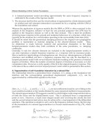
Fig.1 shows turbine mechanical power as a function of rotor speed at various wind speeds.
The power for a certain wind speed is maximum at a certain value of rotor speed called
optimum rotor speed
o
p
t

. This is the speed which corresponds to optimum tip speed
ratio
o

p
t

. In order to have maximum possible power, the turbine should always operate
at
o
p
t

. This is possible by controlling the rotational speed of the turbine so that it always
rotates at the optimum speed of rotation.


Fig. 1. Turbine mechanical power as a function of rotor speed for various wind speeds.
3. Maximum power point tracking control
Wind generation system has been attracting wide attention as a renewable energy source
due to depleting fossil fuel reserves and environmental concerns as a direct consequence of
using fossil fuel and nuclear energy sources. Wind energy, even though abundant, varies

MPPT Control Methods in Wind Energy Conversion Systems
341
continually as wind speed changes throughout the day. Amount of power output from a
WECS depends upon the accuracy with which the peak power points are tracked by the
MPPT controller of the WECS control system irrespective of the type of generator used. The
maximum power extraction algorithms researched so far can be classified into three main
control methods, namely tip speed ratio (TSR) control, power signal feedback (PSF) control
and hill-climb search (HCS) control [2].
The TSR control method regulates the rotational speed of the generator in order to maintain
the TSR to an optimum value at which power extracted is maximum. This method requires
both the wind speed and the turbine speed to be measured or estimated in addition to

requiring the knowledge of optimum TSR of the turbine in order for the system to be able
extract maximum possible power. Fig. 2 shows the block diagram of a WECS with TSR
control.


Fig. 2. Tip speed ratio control of WECS.
In PSF control, it is required to have the knowledge of the wind turbine’s maximum power
curve, and track this curve through its control mechanisms. The maximum power curves
need to be obtained via simulations or off-line experiment on individual wind turbines. In
this method, reference power is generated either using a recorded maximum power curve or
using the mechanical power equation of the wind turbine where wind speed or the rotor
speed is used as the input. Fig. 3 shows the block diagram of a WECS with PSF controller for
maximum power extraction.


Fig. 3. Power signal feedback control.





opt
P

MPPT CONTROLLER

POWER
CONVERTER
TO LOAD
CONTROLLER

P





w
v

TO LOAD
w
v



*


GENERATOR
POWER
CONVERTER
R
opt


CONTROLLE
R








w
v

MPPT CONTROLLER

Fundamental and Advanced Topics in Wind Power
342
The HCS control algorithm continuously searches for the peak power of the wind turbine. It
can overcome some of the common problems normally associated with the other two
methods. The tracking algorithm, depending upon the location of the operating point and
relation between the changes in power and speed, computes the desired optimum signal in
order to drive the system to the point of maximum power. Fig. 4 shows the principle of HCS
control and Fig. 5 shows a WECS with HCS controller for tracking maximum power points.


Fig. 4. HCS Control Principle.

Fig. 5. WECS with hill climb search control.
4. MPPT control methods for PMSG based WECS
Permanent Magnet Synchronous Generator is favoured more and more in developing new
designs because of higher efficiency, high power density, availability of high-energy
permanent magnet material at reasonable price, and possibility of smaller turbine diameter
in direct drive applications. Presently, a lot of research efforts are directed towards
designing of WECS which is reliable, having low wear and tear, compact, efficient, having
low noise and maintenance cost; such a WECS is realisable in the form of a direct drive
PMSG wind energy conversion system.


There are three commonly used configurations for WECS with these machines for
converting variable voltage and variable frequency power to a fixed frequency and fixed
voltage power. The power electronics converter configurations most commonly used for
PMSG WECS are shown in Fig. 6.
PERTURB
d=d+Δd

Y

Δ
P>0

CHANGE
SIGN

N

Generator speed (rad/s
Power ( W )
w
v

x

P



*

x

GENERATO
R

POWER
CONVERTER
TO LOAD
CONTROLLE
R





MPPT CONTROLLER

MPPT Control Methods in Wind Energy Conversion Systems
343

Fig. 6. PMSG wind energy conversion systems

Depending upon the power electronics converter configuration used with a particular
PMSG WECS a suitable MPPT controller is developed for its control. All the three methods
of MPPT control algorithm are found to be in use for the control of PMSG WECS.
4.1 Tip speed ratio control
A wind speed estimation based TSR control is proposed in [3] in order to track the peak
power points. The wind speed is estimated using neural networks, and further, using the
estimated wind speed and knowledge of optimal TSR, the optimal rotor speed command is
computed. The generated optimal speed command is applied to the speed control loop of

the WECS control system. The PI controller controls the actual rotor speed to the desired
value by varying the switching ratio of the PWM inverter. The control target of the inverter
is the output power delivered to the load. This WECS uses the power converter