Extreme Winds in Kuwait Including the Effect of Climate Change

109






















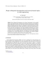
Fig. 20. The predicted extreme gust speed for different return periods from the three
different data groups for the year range 1957-1974, 1975-1992 and 1993-2009.

Fundamental and Advanced Topics in Wind Power

110
5. Conclusions
Extreme wind speed from different directions and for return periods of 10, 25, 50, 100 and
200 years were predicted for five different locations in Kuwait Viz. Kuwait International
Airport (KIA), Kuwait Institute for Scientific Research (KISR), Ras Al-Ardh, Failaka Island
and Al-Wafra. Measured wind speed by the Meteorological office of KIA is used for this
analysis. The wind speeds are measured at 10 m elevation from the ground and the data
value is the average of 10 minutes duration. For KIA location, data is available for 45 years
(From 1962 to 2006). For other locations, measured data is available for about 12 years. The
annual maximum measured wind speed data at KIA location is used as input for the
extreme value analysis for KIA location, whereas the monthly maximum measured wind
speed data is used for other locations. The extreme 10 minute average wind speeds are
predicted based on Gumbel distribution. The wind speed on the earth is dictated by the
spatial gradient of the atmospheric pressure which in turn is governed by the temperature
gradient. The long term climate change affects the temperature gradients and hence the
wind speed. Extreme wind and Gust speed for different return periods is an important
input for safe and economic design of tall structures, power transmission towers, extreme
sand movement in desert and its effects on farm land and related infrastructures. The
updated wind and Gust speed data from Kuwait International Airport (measured data for
54 years from 1957 to 2009) is divided into 3 equal periods, i.e. 1957-1974, 1975-1992, 1993-
2009, each of 18 years duration. Extreme value analysis is also carried out on these three sets
of data to understand the climate change effect on the extreme wind speed. The following
important conclusions are obtained based on the study:-
a. Among the five locations selected for the study,
KIA area is expected to experience the highest wind speed from ENE, ESE, SSE, S, SSW,
SW, WSW, W, and WNW directions.
KISR area is expected to experience the highest wind speed from NW and NNW.
Ras Al-Ardh area is expected to experience the highest wind speed from SE.
Failaka Island is expected to experience the highest wind speed from N, NE and E.
Al-Wafra Island is expected to experience the highest wind speed from NNE.

b. Even though the total land area of Kuwait is about 17,818 km
2
, the variation of space
has very significant effect on the predicted extreme wind speeds in Kuwait. For
example, the 100 year return period wind speed from NW direction varies from 21 m/s
to 27 m/s, when the location is changed from Ras Al-Ardh to KISR. Similarly, the 100
year return period wind speed from SW direction varies from 18 m/s to 31 m/s, when
the location is changed from Al-Wafra to KIA. Similarly, the 100 year return period
wind speed from SE direction varies from 16 m/s to 23 m/s, when the location is
changed from KISR to Ras Al-Ardh.
c. Hence it is strongly recommended that both the effect of wind direction as well as the
location need to be considered, while selecting the probable extreme wind speed for
different return periods for any engineering or scientific applications. The results of the
present study can be useful for the design of tall structures, wind power farms, the
extreme sand transport etc in Kuwait.
d. It is found that the extreme 10 minute average wind speed for 100 year return period is
31.4, 26.5 and 21.8 m/s based on the data set for 1957-1974, 1975-1992, 1993-2009.
e. The extreme gust speed for 100 year return period is 43.1, 38.4 and 33.0 m/s for the
same data sets.

Extreme Winds in Kuwait Including the Effect of Climate Change

111
f. It is clear from the study that long term climate change has reduced the extreme wind
speeds in Kuwait.
g. This information will be useful for various engineering works in Kuwait. Further
investigation is needed to understand why the extreme wind speed for any return
period is reducing when the latest data set is used compared to the oldest data set.
6. Acknowledgements
The authors wish to acknowledge the Kuwait International Airport authorities for providing

the data for the present research work. We are grateful to Warba Insurance Company
(K.S.C.) and Kuwait Foundation for the Advancement of Sciences (KFAS) for the financial
support for the project. We thank Kuwait Institute for Scientific Research, Kuwait for
providing all the facilities for carrying out the research work.
7. References
Abdal,Y., Al-Ajmi, D., Al-Thabia, R., and Abuseil, M., 1986. Recent trends in Wind direction
and Speed in Kuwait. Kuwait Institute for Scientific Research, Report No. 2186,
Kuwait.
Al-Madani, N., Lo, J. M., and Tayfun, M. A., 1989. Estimation of Winds over the Sea from
Land Measurements in Kuwait. Kuwait Institute for Scientific Research, Report No.
3224, Kuwait.
Al-Nassar, W., Al-Hajraf, S., Al-Enizi, A., and Al-Awadhi, L., 2005. Potential Wind Power
Generation in the State of Kuwait, Renewable Energy, Vol. 30, 2149-2161.
Ayyash, S., and Al-Tukhaim, K., 1986. Survey of Wind speed in Kuwait. Kuwait Institute for
Scientific Research, Report No. 2037, Kuwait.
Ayyash, S., and Al-Ammar, J., 1984. Height variation of wind speed in Kuwait. Kuwait
Institute for Scientific Research, Report No. 1402, Kuwait.
Ayyash, S., Al-Tukhaim, K., Al-Jazzaf, M., 1984. Statistical aspects of Wind speed in Kuwait.
Kuwait Institute for Scientific Research, Report No. 1378, Kuwait.
Ayyash, S., Al-Tukhaim, K., Al-Ammar, J., 1985. Assessment of Wind Energy for Kuwait.
Kuwait Institute for Scientific Research, Report No. 1661, Kuwait.
Ayyash, S., Al-Tukhaim, K., Al-Ammar, J., 1984. Characteristics of Wind Energy in Kuwait.
Kuwait Institute for Scientific Research, Report No. 1298, Kuwait.
Climatological Summaries, Kuwait International Airport 1962-1982., 1983. State of Kuwait,
Directorate General of Civil Aviation, Meteorological Department, Climatological
Division.
EPA, 1987. On-Site Meteorological Program Guidance for Regulatory Modeling
Applications, EPA-450/4-87-013, Office of Air Quality Planning and Standards,
Research Triangle Park, NC, 27711
EPA, 1989. Quality Assurance Handbook for Air Pollution Measurement System, Office of

Research and Development, Research Triangle Park, NC, 27711.
Gopalakrishnan, T.C., 1988. Analysis of wind effect in the numerical modeling of flow field.
Kuwait Institute for Scientific Research. Report No.2835-B, Kuwait.
Gomes, L. and Vickery, B.J. (1977). “On the prediction of extreme wind speeds from the
parent distribution”, Journal of Wind Engineering and Industrial Aerodynamics, Vol. 2
No. 1, pp.21-36.

Fundamental and Advanced Topics in Wind Power

112
Gumbel, E.J., 1958. Statistics of Extremes. Columbia University Press, New York.
Kristensen, L., Rathmann, O., and Hansen, S.O. (2000). “Extreme winds in Denmark”,
Journal of Wind Engineering and Industrial Aerodynamics, Vol. 87, No. 2-3, pp.147-166.
IPCC (2007). “Summary for Policymakers, in Climate Change 2007: Impacts, Adaptation and
Vulnerability”. Contribution of Working Group II to the Fourth Assessment Report
of the Intergovernmental Panel on Climate Change, Cambridge University Press,
Cambridge, UK, p. 17.
Milne, R. (1992). “Extreme wind speeds over a Sitka spruce plantation in Scotland”,
Agricultural and Forest Meteorology, Vol. 61, Issues 1-2, pp. 39-53.
Neelamani, S. and Al-Awadi, L., 2004. Extreme wind speed for Kuwait. International
Mechanical Engineering Conference, Dec. 5-8, 2004, Kuwait.
Neelamani, S., Al-Salem, K., and Rakha, K., 2007. Extreme waves for Kuwaiti territorial
waters. Ocean Engineering, Pergaman Press, UK, Vol. 34, Issue 10, July 2007, 1496-
1504.
Neelamani, S., Al-Awadi, L., Al-Ragum, A., Al-Salem, K., Al-Othman, A., Hussein, M. and
Zhao, Y., 2007. Long Term Prediction of Winds for Kuwait, Final report, Kuwait
Institute for Scientific Research, 8731, May 2007.
Simiu, E., Bietry, J., and Filliben, J.J., 1978. Sampling errors in estimation of extreme winds.
Journal of the Structural Division, ASCE, Volume 104, 491-501.
The State Climatologist, 1985. Publication of the American Association of State Standards for

Sensors on Automated Weather Stations, Vol. 9, No.4.
WMO, 1983. Guide to Meteorological Instruments and Methods of Observation, World
Meteorological Organization, No.8, 5
th
Edition, Geneva, Switzerland.
Part 2
Structural and Electromechanical Elements
of Wind Power Conversion

0
Efficient Modelling of Wind Turbine Foundations
Lars Andersen and Johan Clausen
Aalborg University, Department of Civil Engineering
Denmark
1. Introduction
Recently, wind turbines have increased significantly in size, and optimization has led to very
slender and flexible structures. Hence, the Eigenfrequencies of the structure are close to the
excitation frequencies related to e nvironmental loads from wind and waves. To obtain a
reliable estimate of the fatigue life of a wind turbine, the dynamic response of the structure
must be analysed. For this purpose, aeroelastic codes have been developed. Existing codes,
e.g. FLEX by Øye (1996), HAWC by Larsen & Hansen (2004) and FAST by Jonkman & Buhl
(2005), have about 30 degrees of freedom for the structure including tower, nacelle, hub and
rotor; but they do not account for dynamic soil–structure interaction. Thus, the forces on the
structure may be over or underestimated, and the natural frequencies may be determined
inaccurately.
q(t)q(t) Q( f )
ttf
h
t
d

M
f
, J
f
M
n
, J
n
E
t
I
t
, m
t
Rigid
Rigid
Flexible
cylinder
LPM
Layer 1
Layer 2
Half-space
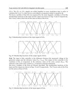
Fig. 1. From prototype to computational model: Wind turbine on a footing over a soil
stratum (left); rigorous model of the layered half-space (centre); lumped-parameter model of
the soil and foundation coupled with finite-element model of the structure (right).
6
2 Will-be-set-by-IN-TECH
Andersen & Clausen (2008) concluded that soil stratification has a significant impact on the
dynamic stiffness, or impedance, of surface footings—even at the very low frequencies
relevant to the first few modes of vibration of a wind turbine. Liingaard et al. (2007)

employed a coupled finite-element/boundary-element model for the analysis of a flexible
bucket foundation, finding a similar variation of the dynamic stiffness in the frequency range
relevant for wind turbines. This illustrated the necessity of implementing a model of the
turbine foundation into the aeroelasic codes that are utilized for design and analysis of the
structure. However, since co mputation speed is of paramount importance, the model of
the foundation should only add few degrees of freedom to the model of the structure. As
proposed by Andersen (2010) and illustr ated in Fig. 1, this may be achieved by fitting a
lumped-parameter model (LPM) to the results of a rigorous analysis, following the concepts
outline by Wolf (1994).
This chapter outlines the methodology for calibration and implementation o f an LPM o f
a wind turbine foundation. Firstly, the f ormulation of rigorous computational models of
foundations is discussed with emphasis on rigid footings, i.e. monolithic gravity-based
foundations. A brief introduction to other types of foundations is given with focus on their
dynamic stiffness properties. Secondly, Sections 2 and 3 provide an in-depth description of an
efficient method for the evaluation of the dynamics stiffness of surface footings of arbitrary
shapes. Thirdly, in Section 4 the concept of consistent lumped-parameter models is presented
and the formulation of a fitting algorithm is discussed. Finally, Section 5 includes a numbe r o f
example results that illustrate the performance of lumped-parameter models.
1.1 Types of foundations and their properties
The gravity footing is the only logical choice of foundation for land-based wind turbines
on residual soils, whereas a direct anchoring may be applied on intact rock. However, for
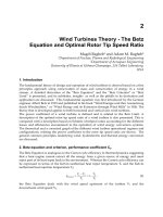
offshore wind turbines a greater variety of possibilities exist. As illustrated in Fig. 2, when the
turbines are taken to greater water depths, the gravity footing may be replaced by a mo nopile,
a bucket foundation or a jacket structure. Another alternative is the tripod which, like the
jacket structure, can be placed o n piles, gravity footings or s pud cans (suction anchors). T he
latter case was studied by Senders (2005). In any case, the choice of foundation type is site
dependent and strongly influenced by the soil properties and the environmental conditions,
i.e. wind, waves, current and ice. Especially, current may involve sediment transport and
scour on sandy and silty seabeds, which m ay lead to the necessity of scour protection around
foundations with a large diameter or width.

Regarding the design of a wind turbine foundation, three limit states must be analysed in
accordance with most codes of practice, e.g. the Eurocodes. For offshore foundations, design
is usually based on the design guidelines provided by the API (2000) o r DNV (2001). Firstly,
the strength and stability of the foundation and subsoil must be high enough to support the
structure in the ultimate limit state (ULS). Secondly, the stiffness of t he foundation should
ensure that the displacements of the structure are below a threshold value in the serviceability
limit state (SLS). Finally, the wind turbine must be analysed regarding failure in the fatigue
limit state (FLS), and this turns out to be critical for large modern o ffshore wind turbines.
The ULS is typically design giving for the foundations of smaller, land-based wind turbines.
In the SLS and FLS the turbine m ay be regarded as fully fixed at the base, leading to a great
simplification of the dynamic system to be analysed. However, as the size of the turbine
increases, soil–structure interaction becomes stronger and due to the high flexibility of the
structure, the first Eigenfrequencies are typically below 0.3 Hz.
116
Fundamental and Advanced Topics in Wind Power
Efficient Modelling of Wind Turbine Foundations 3
(a) (b) (c) (d)
Fig. 2. Different types of wind turbine foundations used offshore a various water depths:
(a) gravity foundation; (b) monopile foundation; (c) monopod bucket foundation and
(d) jacket foundaiton.
An i mproper design may cause resonance d ue to the excitation from wind and waves, leading
to immature failure in the FLS. An accurate prediction of the f atigue life span of a wind turbine
requires a precise estimate of the Eigenfrequencies. This in turn necessitates an adequate
model for the dynamic stiffness of the foundation and subsoil. The formulation of such models
is the focus of such models. The reader is referred to standard text b ooks on geotechnical
engineering for further reading about static behaviour of foundations.
1.2 Computational models of foundations for wind turbines
Several methods can be used to evaluate the dynamic stiffness of footings resting on
the surface of the ground or embedded within the soil. Examples include analytic,
semi-analytic or semi-empirical methods as proposed by Luco & Westmann (1971), Luco

(1976), Krenk & Schmidt (1981), Wong & Luco (1985), Mita & Luco (1989), Wolf (1994) and
Vrettos (1999) as well as Andersen & Clausen (2008). Especially, torsional motion of
footings was studied by Novak & Sachs (1973) and Veletsos & Damodaran Nair (1974) as
well as Avilés & Pérez-Rocha (1996). Rocking and horizontal sliding motion of footings was
analysed by Veletsos & Wei (1971) and Ahmad & Rupani (1999) as well as Bu & Lin (1999).
Alternatively, numerical analysis may be conducted using the finite-element method and the
boundary-element method. See, for example, the work by Emperador & Domínguez (1989)
and Liingaard et al. (2007).
For monopiles, analyses are usually performed by means of the Winkler approach in which
the pile is continuously supported by springs. The nonlinear soil stiffness in the axial direction
along the shaft is described by t–z curves, whereas the horizontal soil resistance along the shaft
is provided by p–y curves. Here, t and p is the resulting force per unit length in the vertical
and horizontal directions, respectively, whereas z and y are the corresponding displacements.
For a pile loaded vertically in compression, a similar model can be formulated for the tip
117
Efficient Modelling of Wind Turbine Foundations
4 Will-be-set-by-IN-TECH
resistance. More information about these methods can be found in the design guidelines by
API (2000) and D NV (2001).
Following this approach, El Naggar & Novak (1994a;b) formulated a model for vertical
dynamic loading of pile foundations. Further studies regarding the axial response were
conducted by Asgarian et al. (2008), who studied pile–soil interaction for an offshore jacket,
and Manna & Baidya ( 2010), who compared computational and experimental re sults. In
a similar manner, El Naggar & Novak (1995; 1996) studied monopiles subject to horizontal
dynamic excitation. More work along this line is attributed to El Naggar & Bentley (2000),
who formulated p–y curves for dynamic pile–soil interaction, and Kong et al. (2006), who
presented a simplified method including the effect of separation between the pile and the
soil. A further development of Winkler models for nonlinear dynamic soil behaviour was
conducted by Allotey & El Naggar (2008). Alternatively, the performance of mononpiles
under cyclic lateral loading was studied by Achmus et al. (2009) using a finite-element model.

Gerolymos & Gaze tas (2006a;b;c) developed a Winkler model for static and dynamic analysis
of caisson foundations fully embedded in linear or nonlinear soil. Further research regarding
the formulation of simple models for dynamic response of bucket foundations was carried
out by Varun et al. (2009). The concept of the monopod bucket foundation has been d escribed
by Houlsby et al. (2005; 2006) as well as Ibsen (2008). Dynamic analysis of such foundations
were performed by Liingaard et al. (2007; 2005) and Liingaard (2006) as well as Andersen et al.
(2009). The latter work will be further described by the end of this chapter.
2. Semi-analytic model of a layered ground
This section provides a thorough explanation o f a semi-analytical model that may be a pplied
to evaluate the response of a layered, or stratified, ground. The derivation follows the original
work by Andersen & Clausen (2008). The fundamental assumption is that the ground may be
analysed as a horizontally layered half-space with each soil layer consisting of a homogeneous
linear viscoelastic material. In Section 3 the model of t he ground will be used as a b asis for
the development of a numerical method providing the dynamic stiffness of a foundation over
a stratum. Finally, in Section 5 this method will be applied to the analysis of gravity-based
foundations for offshore wind turbines.
2.1 Response of a layered half-space
The surface displacement in time domain and in Cartesian space is denoted u
10
i
(x
1
, x
2
, t)=
u
i
(x
1
, x

2
,0,t). Likewise the surface traction, or the load on the free surface, will be denoted
p
10
i
(x
1
, x
2
, t)=p
i
(x
1
, x
2
,0,t). An explanation of the double superscript 10 is given in the next
subsection. Here it is just noted that superscript 10 refers to the top of the half-space.
Further, let g
ij
(x
1
− y
1
, x
2
− y
2
, t − τ) be the Green’s function relating the displacement at
the observation point
(x

1
, x
2
,0) to the traction applied at the source point (y
1
, y
2
,0).Both
points are situated on the surface of a stratified half-space with horizontal interfaces. The
total displacement at the point
(x
1
, x
2
,0) on the surface of the half-space is then found as
u
10
i
(x
1
, x
2
, t)=

t
−∞

∞
−∞


∞
−∞
g
ij
(x
1
−y
1
, x
2
−y
2
, t −τ)p
10
j
(y
1
, y
2
, τ) dy
1
dy
2
dτ.(1)
The displacement at any point on the surface of the half-space and at any instant of time may
be evaluated by means of Eq. (1). However, this requires the existence of the Green’s function
g
ij
(x
1

−y
1
, x
2
−y
2
, t −τ), which may be interpreted as the dynamic flexibility. Unfortunately,
118
Fundamental and Advanced Topics in Wind Power
Efficient Modelling of Wind Turbine Foundations 5
a closed-form solution cannot be established for a layered half-space, and in practice the
temporal–spatial solution expressed by Eq. (1) is inapplicable.
Assuming that the response of the stratum is linear, the analysis may be carried out in the
frequency domain. The Fourier transformation of the surface displacements with respect to
time is defined as
U
10
i
(x
1
, x
2
, ω)=

∞
−∞
u
10
i
(x

1
, x
2
, t)e
−iωt
dt (2)
with the inverse Fourier transformation given as
u
10
i
(x
1
, x
2
, t)=
1
2π

∞
−∞
U
10
i
(x
1
, x
2
, ω)e
iωt
dω.(3)

Likewise, a relationship can be established between the surface load p
10
i
(x
1
, x
2
, t) and its
Fourier transform P
10
i
(x
1
, x
2
, ω), and similar t ransformation rules apply to the Green’s
function, i.e. between g
ij
(x
1
− y
1
, x
2
− y
2
, t −τ) and G
ij
(x
1

− y
1
, x
2
− y
2
, ω). It then follows
that
U
10
i
(x
1
, x
2
, ω)=

∞
−∞

∞
−∞
G
ij
(x
1
−y
1
, x
2

−y
2
, ω)P
10
j
(y
1
, y
2
, ω)dy
1
dy
2
,(4)
reducing the problem to a purely spatial convolution.
Further, assuming that all interfaces are horizontal, a transformation is carried out from the
Cartesian space domain description into a horizontal wavenumber domain. This is done by a
double Fourier transformation in the form
U
10
i
(k
1
, k
2
, ω)=

∞
−∞


∞
−∞
U
10
i
(x
1
, x
2
, ω)e
−i(k
1
x
1
+k
2
x
2
)
dx
1
dx
2
,(5)
where the double inverse Fourier transformation is defined by
U
10
i
(x
1

, x
2
, ω)=
1
4π
2

∞
−∞

∞
−∞
U
10
i
(k
1
, k
2
, ω)e
i(k
1
x
1
+k
2
x
2
)
dk

1
dk
2
.(6)
By a similar transformation of the surface traction and the Green’s function, Eq. (4) finally
achieves the form
U
10
i
(k
1
, k
2
, ω)=G
ij
(k
1
, k
2
, ω)P
10
j
(k
1
, k
2
, ω).(7)
This equation has the advantage when compared to the previous formulation in space and
time domain, that no convolution has to be carried out. Thus, the displacement amplitudes
in the frequency–wavenumber domain are related directly to the traction amplitudes for a

given set of the circular freqeuncy ω and the horizontal wavenumbers k
1
and k
2
via the
Green’s function tensor
G
ij
(k
1
, k
2
, ω). When the load in the time domain varies harmonically
in the form p
10
i
(x
1
, x
2
, t)=P
i
(x
1
, x
2
)e
iωt
, the solution simplifies, since no inverse Fourier
transformation over the frequency is necessary.

G
ij
(k
1
, k
2
, ω) must only be evaluated at a
single frequency.
The main advantage of the description in the frequency–horizontal wavenumber domain is
that a solution for the stratum may be found analytically. In the following subsections, the
derivation of
G
ij
(k
1
, k
2
, ω) is described. As mentioned above, the derivation is based on the
assumption that the material within each individual layer is linear elastic, homogeneous and
isotropic. Further, material dissipation is confined to hysteretic damping, which has been
found to be a r easonably accurate model for materials such as soil, even if the model is invalid
from a physical point of view.
119
Efficient Modelling of Wind Turbine Foundations
6 Will-be-set-by-IN-TECH
2.2 Flexibility matrix for a single soil layer
The stratum consists of J horizontally bounded layers, each defined by the Young’s modulus
E
j
, the Poisson ratio ν

j
, the mass density ρ
j
and the loss factor η
j
. Further, the layers have the
depths h
j
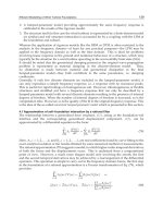
, j = 1, 2, , J. Thus, the equations of motion for each layer may ad vantageously be
established in a coordinate system with the local x
3
-coordinate x
j
3
defined with the positive
direction downwards so that x
j
3
∈ [0, h
j
], see Fig. 3.
2.2.1 Boundary conditions for displacements and stresses at an interface
In the frequency domain, and in terms of the horizontal wavenumbers, the displacements a t
the top and at the bottom of the jth layer are given, respectively, as
U
j0
i
(k
1
, k

2
, ω)=U
i
(k
1
, k
2
, x
j
3
= 0, ω), U
j1
i
(k
1
, k
2
, ω)=U
i
(k
1
, k
2
, x
j
3
= h
j
, ω).(8)
The meaning of the double superscript 10 applied in the definition of the flexibility or

Green’s function in the previous section now becomes somewhat clearer. Thus
U
10
i
are the
displacement components at the top of the uppermost layer which coincides with the surface
of the half-space. The remaining layers are counted downwards with j
= J referring to the
bottommost layer. If an underlying half-space is present, its material properties are i dentified
by index j
= J + 1.
Similar to Eq. (8) for the displacements, the traction at the top and bottom of layer j are
P
j0
i
(k
1
, k
2
, ω)=P
i
(k
1
, k
2
, x
j
3
= 0, ω), P
j1

i
(k
1
, k
2
, ω)=P
i
(k
1
, k
2
, x
j
3
= h
j
, ω).(9)
The quantities defined in Eqs. (8) and (9) may advantageously be stored i n ve ctor form as
S
j0
=

U
j0
P
j0

,
S
j1

=

U
j1
P
j1

, (10)
where
U
j0
= U
j0
(k
1
, k
2
, ω) is the column vector with the components U
j0
i
, i = 1, 2, 3, etcetera.
x
1
x
2
x
3
, x
j
3

O
O
j
h
j
Layer j
Fig. 3. Global and local coordinates for layer j with the depth h
j
.The(x
1
, x
2
, x
3
)-coordinate
system has the origin O, whereas the local
(x
1
, x
2
, x
j
3
)-coordinate system has the origin O
j
.
120
Fundamental and Advanced Topics in Wind Power
Efficient Modelling of Wind Turbine Foundations 7
2.2.2 Governing equations for wave propagation in a soil layer

In the time domain, and in terms of Cartesian coordinates, the equations of motion for the
layer are given in terms of the Cauchy equations, which in the absence of body forces read
∂
∂x
k
σ
j
ik
(x
1
, x
2
, x
j
3
, t)=ρ
j
∂
2
∂t
2
u
j
i
(x
1
, x
2
, x
j

3
, t), (11)
where σ
j
ik
(x
1
, x
2
, x
j
3
, t) is the Cauchy stress tensor. On any part of the boundary, i.e. on the top
and bottom of the layer, Dirichlet or Neumann conditions apply as defined by Eqs. (8) and
(9), respectively. Initial co nditions are of no interest in the present case, since the steady state
solution is to be found.
Assuming hysteretic material dissipation defined by the loss f actor η
j
, the dynamic s tiffness of
the homogeneous and isotropic material may conveniently be described in terms of complex
Lamé constants defined as
λ
j
=
ν
j
E
j

1

+ isign(ω)η
j


1
+ ν
j

1
−2ν
j

, μ
j
=
E
j

1
+ isign(ω)η
j
)

2

1 + ν
j

. (12)
The sign function ensures that the material damping is positive in the entire frequency range

ω
∈ [−∞; ∞] involved in the inverse Fourier transformation (3).
Subsequently, the stress amplitudes

σ
j
ik
(x
1
, x
2
, x
j
3
, ω) may be expressed i n terms of the dilation
amplitudes

Δ
j
(x
1
, x
2
, x
j
3
, ω), and the infinitesimal strain tensor amplitudes

ε
j

ik
(x
1
, x
2
, x
j
3
, ω),

σ
j
ik
(x
1
, x
2
, x
j
3
, ω)=λ
j

Δ
j
(x
1
, x
2
, x

j
3
, ω)δ
ik
+ 2μ
j

ε
j
ik
(x
1
, x
2
, x
j
3
, ω), (13)
where δ
ij
is the Kronecker delta; δ
ij
= 1fori = j and δ
ij
= 0fori = j. Further, the following
definitions apply:

Δ
j
(x

1
, x
2
, x
j
3
, ω)=
∂
∂x
k
U
j
k
(x
1
, x
2
, x
j
3
, ω), (14)

ε
j
ik
(x
1
, x
2
, x

j
3
, ω)=
1
2

∂
∂x
i
U
j
k
(x
1
, x
2
, x
j
3
, ω)+
∂
∂x
k
U
j
i
(x
1
, x
2

, x
j
3
, ω)

. (15)
It is noted that ∂/∂x
j
3
= ∂/∂x
3
, since the local x
j
3
-axes have the same positive direction as the
global x
3
-axis.
Inserting Eqs. (12) to (15) into the Fourier transformation of the Cauchy equation given by
Eq. (11), the Navier equations in the frequency domain are achieved:

λ
j
+ μ
j

∂

Δ
j

∂x
i
+ μ
j
∂
2
U
j
i
∂x
k
∂x
k
= −ω
2
ρ
j
U
j
i
. (16)
Applying the double Fourier transformation over the horizontal Cartesian coordinates as
defined by Eq. (5), the Navier equations in the frequency–wavenumber domain become

λ
j
+ μ
j

ik

i
Δ
j
+ μ
j

d
2
dx
2
3
−k
2
1
−k
2
2

U
j
i
= −ω
2
ρ
j
U
j
i
, i = 1, 2, (17a)


λ
j
+ μ
j

d
Δ
j
dx
3
+ μ
j

d
2
dx
2
3
−k
2
1
−k
2
2

U
j
3
= −ω
2

ρ
j
U
j
3
, (17b)
121
Efficient Modelling of Wind Turbine Foundations
8 Will-be-set-by-IN-TECH
where Δ
j
= Δ
j
(k
1
, k
2
, x
j
3
, ω) is the double Fourier transform of

Δ
j
(x
1
, x
2
, x
j

3
, ω) with respect t o
the horizontal Cartesian coordinates x
1
and x
2
. Obviously,
Δ
j
(k
1
, k
2
, x
j
3
, ω)=ik
1
U
j
1
(k
1
, k
2
, x
j
3
, ω)+ik
2

U
j
2
(k
1
, k
2
, x
j
3
, ω)+
dU
j
3
(k
1
, k
2
, x
j
3
, ω)
dx
3
. (18)
Equations ( 17a) and (17b) are ordinary differential equations in x
3
. When the boundary val ues
at the top and the bottom of the layer expressed in Eqs. (8) and (9) are known, an analytical
solution may be found as will be discussed below.

2.2.3 The solution for compression waves in a soil layer
The phase velocities of compression and shear waves, or P- and S-waves, are identified as
c
P
=

λ
j
+ 2μ
j
ρ
j
, c
S
=

μ
j
ρ
j
, (19)
respectively. I t is noted that the phase velocities are complex when material damping is
present. Further, in the frequency domain, the P- and S-waves in layer j are associated with
the wavenumbers k
j
P
and k
j
S
,

{k
j
P
}
2
=
ω
2
{c
j
P
}
2
, {k
j
S
}
2
=
ω
2
{c
j
S
}
2
. (20)
Introducing the p arameters α
j
P

and α
j
S
as the larger of the roots to
{α
j
P
}
2
= k
2
1
+ k
2
2
−{k
j
P
}
2
, {α
j
S
}
2
= k
2
1
+ k
2

2
−{k
j
S
}
2
, (21)
Eqs. (17a) and (17b) may conveniently be recast as

λ
j
+ μ
j

ik
i
Δ
j
+ μ
j

d
2
U
j
i
dx
2
3
−{α

j
S
}
2
U
j
i

= 0, i = 1, 2, (22a)

λ
j
+ μ
j

d
Δ
j
dx
3
+ μ
j

d
2
U
j
3
dx
2

3
−{α
j
S
}
2
U
j
3

= 0. (22b)
Equation (22a) is now multiplied with ik
i
and Eq. (22b) is differentiated with respect to x
3
.
Adding the three resulting equations and making use of Eq. (18), an equation for the dilation
is obtained in the form

λ
j
+ μ
j


d
2
dx
2
3

−k
2
1
−k
2
2

Δ
j
+ μ
j

d
2
dx
2
3
−{α
j
S
}
2

Δ
j
= 0 ⇒

λ
j
+ 2μ

j


d
2
dx
2
3
−k
2
1
−k
2
2

Δ
j
+ μ
j

k
2
1
+ k
2
2
−{α
j
S
}

2

Δ
j
= 0 ⇒

λ
j
+ 2μ
j


d
2
dx
2
3
−k
2
1
−k
2
2

Δ
j
+ μ
j
{k
j

S
}
2
Δ
j
= 0. (23)
122
Fundamental and Advanced Topics in Wind Power
Efficient Modelling of Wind Turbine Foundations 9
The last derivation follows from Eq. (21). Further, Eqs. (19) and (20) involve that
μ
j
{k
j
S
}
2
=

λ
j
+ 2μ
j

{k
j
P
}
2
. (24)

Inserting this result i nto Eq. (23), and once again making use of Eq. (21), we finally arrive at
the ordinary homogenous differential equation
d
2
Δ
j
dx
2
3
−{α
j
P
}
2
Δ
j
= 0, (25)
which has the full solution
Δ
j
= a
j
1
e
α
j
P
x
j
3

+ a
j
2
e
−α
j
P
x
j
3
. (26)
Here a
j
1
and a
j
2
are i ntegration constants that follow f rom the boundary conditions. Physically,
the two parts of the solution (26) describe the decay of P-waves travelling in the negative and
positive x
3
-direction, respectively, i.e. P-waves moving up and down in the layer.
2.2.4 The solution for compression and shear waves in a soil layer
Insertion of the solution (26) into Eqs. (22a) and (22b) leads to three equations for the
displacement amplitudes:
d
2
U
j
i

dx
2
3
−{α
j
S
}
2
U
j
i
= −

λ
j
μ
j
+ 1

ik
i

a
j
1
e
α
j
P
x

j
3
+ a
j
2
e
−α
j
P
x
j
3

, i
= 1, 2, (27a)
d
2
U
j
3
dx
2
3
−{α
j
S
}
2
U
j

3
= −

λ
j
μ
j
+ 1

α
j
P

a
j
1
e
α
j
P
x
j
3
− a
j
2
e
−α
j
P

x
j
3

. (27b)
Solutions to Eqs. (27a) and (27b) are found in the form
U
j
1
= U
j
1,c
+ U
j
1,p
= b
j
1
e
α
j
S
x
j
3
+ b
j
2
e
−α

j
S
x
j
3
+ b
j
3
e
α
j
P
x
j
3
+ b
j
4
e
−α
j
P
x
j
3
, (28a)
U
j
2
= U

j
2,c
+ U
j
2,p
= c
j
1
e
α
j
S
x
j
3
+ c
j
2
e
−α
j
S
x
j
3
+ c
j
3
e
α

j
P
x
j
3
+ c
j
4
e
−α
j
P
x
j
3
, (28b)
U
j
3
= U
j
3,c
+ U
j
3,p
= d
j
1
e
α

j
S
x
j
3
+ d
j
2
e
−α
j
S
x
j
3
+ d
j
3
e
α
j
P
x
j
3
+ d
j
4
e
−α

j
P
x
j
3
, (28c)
where the subscripts c and p denote the complimentary and the particular solutions,
respectively. These include S- and P-wave terms, respectively. Like a
j
1
and a
j
2
, c
j
1
, c
j
2
,etc.are
integration constants given by the boundary conditions at the top and the bottom of layer j.
Apparently, the full solution has fourteen integration constants. However, a comparison of
Eqs. (18) and (26) reveals that
Δ
j
(k
1
, k
2
, x

j
3
, ω)=ik
1
U
j
1
+ ik
2
U
j
2
+
dU
j
3
dx
3
= a
j
1
e
α
j
P
x
j
3
+ a
j

2
e
−α
j
P
x
j
3
. (29)
By insertion of the complementary solutions, i.e. the first two terms in Eqs. (28a) to (28c), into
Eq. (29) it immediately follows that
d
j
1
= −

ik
1
α
j
S
b
j
1
+
ik
2
α
j
S

c
j
1

, d
j
2
=
ik
1
α
j
S
b
j
2
+
ik
2
α
j
S
c
j
2
. (30)
123
Efficient Modelling of Wind Turbine Foundations
10 Will-be-set-by-IN-TECH
functions of different powers are orthogonal. A further reduction of the number of i ntegration

constants is achieved by insertion of the particular solutions into the respective differential
equations (27a) and (27b). Thus, after a few manipulations it may be shown that
b
j
3
= −
ik
1
{k
j
P
}
2
a
j
1
, c
j
3
= −
ik
2
{k
j
P
}
2
a
j
1

, d
j
3
= −
α
j
P
{k
j
P
}
2
a
j
1
, (31a)
b
j
4
= −
ik
1
{k
j
P
}
2
a
j
2

, c
j
4
= −
ik
2
{k
j
P
}
2
a
j
2
, d
j
4
=+
α
j
P
{k
j
P
}
2
a
j
2
, (31b)

where use has been made of the fact that
λ
j
+ μ
j
μ
j

{α
j
S
}
2
−{α
j
P
}
2

=
{
c
j
P
}
2
−{c
j
S
}

2
{c
j
S
}
2

{k
j
P
}
2
−{k
j
S
}
2

=
{
k
j
S
}
2
−{k
j
P
}
2

{k
j
P
}
2

{k
j
P
}
2
−{k
j
S
}
2

= −
1
{k
j
P
}
2
,
which follows from the definitions given in Eqs. (19) to (21). Thus, eventually only six of
the o riginal fourteen integration constants are independent, namely a
j
1
, a

j
2
, b
j
1
, b
j
2
, c
j
1
and
c
j
2
. As already mentioned, the terms including a
j
1
and a
j
2
represent P-waves moving up and
down in layer j. Inspection of Eqs. (28a) to (28c) reveals that the b
j
1
and b
j
2
terms represent
S-waves that are polarized in the x

1
-direction and which are moving up and down in the
layer, respectively. Similarly, the c
j
1
and c
j
2
terms describe the contributions from S-waves
polarized in the x
2
-direction and travelling up and down in the layer, respectively. It becomes
evident that the previously defined quantities α
j
P
and α
j
S
may be interpreted as exponential
decay coefficients of P- and S-waves, respectively. When k
1
and k
2
are both small, α
j
P
and α
j
S
turn into “wavenumbers”, as they become imaginary, cf. Eq. (21).

Once the displacement field is known, the stress components on any plane orthogonal to the
x
j
3
-axis may be found from Eq. (13) by letting index k = 3. The full solution for displacements,
U
j
, and traction, P
j
, may then be written in matrix form as
S
j
=

U
j
P
j

= A
j
E
j
b
j
, b
j
=

a

j
1
b
j
1
c
j
1
a
j
2
b
j
2
c
j
2

T
, (32)
where E
j
is a matrix of dimension (6 × 6). Only the diagonal terms
E
j
11
= e
α
j
P

x
j
3
, E
j
22
= E
j
33
= e
α
j
S
x
j
3
, E
j
44
= e
−α
j
P
x
j
3
, E
j
55
= E

j
66
= e
−α
j
S
x
j
3
, (33)
are nonzero. A
j
is a matrix of dimension (6 × 6), the components of which follow from
Eqs. (28) to (31) and (13). The computation of matrix A
j
is further discussed below. Finally,
the displacements and the traction at the two boundaries of layer j may be expressed as
S
j0
= A
j0
b
j
, A
j0
= A
j
, (34a)
S
j1

= e
α
j
P
h
j
A
j1
b
j
, A
j1
= A
j0
D
j
. (34b)
Here D
j
a (6 ×6) matrix with the nonzero components
D
j
11
= 1, D
j
22
= D
j
33
= e

(α
j
S
−α
j
P
)h
j
, D
j
44
= e
−2α
j
P
h
j
, D
j
55
= D
j
66
= e
−(α
j
P
+α
j
S

)h
j
, (35)
124
Fundamental and Advanced Topics in Wind Power
Efficient Modelling of Wind Turbine Foundations 11
found by evaluation of the matrix e
−α
j
P
x
j
3
E
j
at x
j
3
= h
j
. Equations (34a) and (34b) may be
combined in order to eliminate vector b
j
which contains unknown integration constants. This
provides a transfer matrix for the layer as proposed by Thomson (1950) and Haskell (1953),
S
j1
= e
α
j

P
h
j
A
j1
[A
j0
]
−1
S
j0
, (36)
forming a relationship between the displacements and the traction at the top and the bottom
of a single layer.
The derivation of Eq. (36) h as been based on the assumption that ω
> 0. W hen a static load
is applied, the circular frequency is ω
= 0, whereby the wavenumbers of the P- and S-waves,
i.e. k
j
P
and k
j
S
defined by Eq. (20), become zero and the integration constants b
j
3
etc. given in
Eq. (31) are undefined. Hence, the solution given in the previous section does not apply in the
static case. However, for any practical purposes a useful approximation can be established f or

the static case by employing a low value of ω in the evaluation of
S
j1
.
2.3 Assembly of multiple layers
At an interface between two layers, the d isplacements should be continuous and there should
be equilibrium of the traction. This may be expressed as
S
j0
= S
j−1,1
, j = 2, 3, , J,i.e.the
quantities at the top of layer j are equal to those at the bottom of layer j
−1. Proceeding in this
manner, Eq. (36) for the single layer may be rewritten for a system of J layers,
S
J1
= e
Σα
A
J1
[A
10
]
−1
A
J−1,1
[A
J−1,0
]

−1
···A
11
[A
10
]
−1
S
10
, Σα =
J
∑
j=1
α
j
P
h
j
. (37)
Introducing the transfer matrix T defined as
T
=

T
11
T
12
T
21
T

22

= A
J1
[A
J0
]
−1
A
J−1,1
[A
J−1,0
]
−1
···A
11
[A
10
]
−1
, (38)
Equation (37) may in turn be written as
S
J1
= e
Σα
TS
10
,or


U
J1
P
J1

= e
Σα

T
11
T
12
T
21
T
22


U
10
P
10

, Σα
=
J
∑
j=1
α
j

P
h
j
. (39)
This establishes a relationship between the traction and the displacements at the free surface
of the half-space and the equivalent quantities at the bottom of the stratum as originally
proposed by Thomson (1950) and Haskell (1953).
2.4 Flexibility of a homogeneous or stratified ground
A stratified ground consisting of multiple soil layers may overlay bedrock. On the surface of
the be drock, the displacements are identically e qual to zero and thus, by insertion into Eq. (39),

U
J1
P
J1

=

0
P
J1

= e
Σα

T
11
T
12
T

21
T
22


U
10
P
10

. (40)
The first three rows of this matrix equation provide the identity
U
10
= G
rf
P
10
, G
rf
= −T
−1
11
T
12
. (41)
125
Efficient Modelling of Wind Turbine Foundations
12 Will-be-set-by-IN-TECH
G

rf
= G
rf
(k
1
, k
2
, ω) is the flexibility matrix for a stratum over a rigid bedrock. It is
observed that the exponential function of the power Σα,definedinEq.(39),vanishesinthe
formulation provided by Eq. (41). This is a great advantage from a computational point of
view, since e
Σα
becomes very large for strata of great depths, which may lead to problems on
a computer—even when double precision complex variables are employed.
Alternatively to a rigid bedrock, a half-space may be present underneath the stratum
consisting of J layers. In this context, the material properties etc. of the half-space will be
assigned the superscript J
+ 1. The main d ifference between a semi-infinite half-space and a
layer of finite depth is that only an upper boundary is present, i.e. the boundary situated at
x
J+1
3
= 0. Since the material is assumed to be h omogeneous, no reflection o f waves will take
place inside the half-space. Further assuming that no sources are present in the interior of the
half-space, only outgoing, i.e. downwards propagating, waves can be present. Dividing the
matrices A
j
and E
j
for a layer of finite depth, cf. Eq. (32), into four quadrants, and the column

vector b
j
into two sub-vectors,
A
j
=

A
j
11
A
j
12
A
j
21
A
j
22

, E
j
=

E
j
11
E
j
12

E
j
21
E
j
22

, b
j
=

b
j
1
b
j
2

, (42)
it is evident that only half of the solution applies to the half-space, i.e.
S
J+1
=

U
J+1
P
J+1

=


A
J+1
12
A
J+1
22

E
J+1
22
b
J+1
2
, b
J+1
2
=

a
J+1
2
b
J+1
2
c
J+1
2

T

. (43)
The terms including the integration constants a
J+1
1
, b
J+1
1
and c
J+1
1
are physically invalid as
they correspond to waves incoming from x
J+1
3
= ∞, i.e. from infinite depth.
From Eq. (43), the traction on the interface between the bottommost layer and the half-space
may be expressed in terms of the corresponding displacements by solution of
U
J+1
= A
J+1
12
[A
J+1
22
]
−1
P
J+1
. (44)

The matrix E
J+1
22
reduces to the identity matrix of order 3, since all the exponential terms are
equal to 1 for x
J+1
3
= 0.
Firstly, if no layers are present in the model of the stratum, J
= 0 and it immediately follows
from Eq. (44) that Eq. (7), written in matrix form, becomes
U
10
= G
hh
P
10
, G
hh
= A
10
12
[A
10
22
]
−1
, (45)
where it is noted that the flexibility matrix for the homogeneous half-space
G

hh
=
G
hh
(k
1
, k
2
, ω) is given in the horizontal wavenumber–frequency domain.
Secondly, when J layers overlay a homogeneous half-space, continuity of the displacements,
equilibrium of the traction and application of Eq. (44) provide
U
J1
= U
J+1,0
= A
J+1
12
[A
J+1
22
]
−1
P
J+1,0
= A
J+1
12
[A
J+1

22
]
−1
P
J1
. (46)
Insertion of this result into Eq. (39) leads to the following system of equations:

U
J1
P
J1

=

A
J+1
12
[A
J+1
22
]
−1
P
J1
P
J1

= e
Σα


T
11
T
12
T
21
T
22


U
10
P
10

. (47)
126
Fundamental and Advanced Topics in Wind Power
Efficient Modelling of Wind Turbine Foundations 13
From the bottommost three rows of the matrix equation, an expression of P
J1
is obtained
which may be inserted into the first three equations. This leads to the solution
U
10
= G
lh
P
10

, (48)
where the flexibility matrix for the layered half-space
G
lh
= G
lh
(k
1
, k
2
, ω) is given by
G
lh
=

A
J+1
12
[A
J+1
22
]
−1
T
21
−T
11

−1


T
12
−A
J+1
12
[A
J+1
22
]
−1
T
22

. (49)
Again the exponential function disappears. In the following, no distinction is made between
G
rf
, G
hh
and G
lh
. The common notation G will be employed, independent of the type of
subsoil model.
2.5 Optimising the numerical evaluation o f the Green’s function
In order to obtain a solution in Cartesian space, a double inverse Fourier transformation over
the horizontal wavenumbers is necessary as outlined by Eq. (6). A direct approach involves
the evaluation of
G for numerous combinations of k
1
and k

2
, leading to long computation
times. However, as described in this subsection, a considerable reduction of the computation
time can be achieved.
2.5.1 C omputation of the matrices A
j0
and A
j1
The computation of the transfer matrix T involves inversion of the matrices A
j0
, j = 1, 2, , J.
Further, the flexibility matrix
G(k
1
, k
2
, ω) has to be evaluated for all combinations (k
1
, k
2
)
before the tr ansformation given by Eq. (6) may be applied. However, as pointed out by
Sheng et al. (1999), the evaluation of A
j
, and therefore also the Green’s function matrix G,
is particularly simple along the line defined by k
1
= 0. To take advantage of this, a coordinate
transformation is introduced in the form
⎡

⎣
k
1
k
2
x
3
⎤
⎦
= R(ϕ)
⎡
⎣
γ
α
x
3
⎤
⎦
, R
(ϕ)=
⎡
⎣
sin ϕ cos ϕ 0
−cos ϕ sin ϕ 0
001
⎤
⎦
. (50)
This corresponds to a rotation of
(k

1
, k
2
, x
3
)-basis by the angle ϕ −π/2 around the x
3
-axis as
illustrated in Fig. 4. It follows from Eq. (50) that R
ij
(ϕ)=R
ji
(π − ϕ), which in matrix–vector
notation corresponds to
{R(ϕ)}
T
= R(π − ϕ).
For any combination of k
1
and k
2
,theangleϕ is now defined so that γ = 0. The relationship
between the coordinates in the two systems of reference is then given by
k
1
= α cos ϕ, k
2
= α sin ϕ, α =

k

2
1
+ k
2
2
, tan ϕ =
k
2
k
1
, γ = 0. (51)
The computational advantage of this particular orientation of the
(γ, α, x
3
)-coordinate system
is twofold. Firstly, the flexibility matrix may be evaluated along a line r ather than over an
area, and for any other combination of the wavenumbers, the Green’s function m atrix can be
computed as
G(k
1
, k
2
, ω)=R(ϕ)

G{R(ϕ)}
T
or G
ik
(k
1

, k
2
, ω)=R
il
(ϕ)

G
lm
R
km
(ϕ). (52)
127
Efficient Modelling of Wind Turbine Foundations
14 Will-be-set-by-IN-TECH
k
1
k
2
x
3
γ
α
ϕ
Fig. 4. Definition of the (k
1
, k
2
, x
3
)-and(γ, α, x

3
)-coordinate systems.
Here

G =

G(α, ω)=G(0, α, ω). Secondly, the matrices A
j0
and A
j1
—and therefore also A
J+1
12
and A
J+1
22
—simplify significantly when one of the wavenumbers is equal to zero. Thus, when
k
1
= γ = 0, k
2
= α and ω = 0,

A
j0
= A
j0
(0, α, ω)=
⎡
⎢

⎢
⎢
⎢
⎢
⎢
⎢
⎢
⎣
010010

A
j0
21
01

A
j0
21
01

A
j0
31
0

A
j0
33
−


A
j0
31
0 −

A
j0
33
0

A
j0
42
00−

A
j0
42
0

A
j0
51
0

A
j0
53
−


A
j0
51
0 −

A
j0
53

A
j0
61
0

A
j0
63

A
j0
61
0

A
j0
63
⎤
⎥
⎥
⎥

⎥
⎥
⎥
⎥
⎥
⎦
, (53a)
where

A
j0
21
= −iα/{k
j
P
}
2
,

A
j0
31
= −α
j
P
/{k
j
P
}
2

,

A
j0
33
= −iα/α
j
S
, (53b)

A
j0
42
= α
j
S
μ
j
,

A
j0
51
= −2iμ
j
α
j
P
α/{k
j

P
}
2
,

A
j0
53
= μ
j
(α
2
/α
j
S
+ α
j
S
), (53c)

A
j0
61
= −μ
j

{k
j
S
}

2
+ 2{α
j
S
}
2

/
{k
j
P
}
2
,

A
j0
63
= −2iμ
j
α. (53d)
At the bottom of the layer, the corresponding matrix is evaluated as

A
j1
=

A
j0
D

j
,wherethe
components of the matrix D
j
are given b y Eq. (35). A result of the many zeros in

A
j0
and

A
j0
0
is
that the matrices can be inverted analytically. This may re duce computation time significantly.
The inversion of

A
j0
and

A
j0
0
is straightforward and will not be treated further.
Especially, for a homogeneous half-space, possibly underlying a stratum, the matrices

A
J+1,0
12

and

A
J+1,0
22
are readily o btained from the leftmost three columns of

A
j0
,whereas

A
j1
is
obtained as

A
j1
=

A
j0
D
j
(54)
in accordance with Eq. (34b). Note that D
j
is symmetric in the (k
1
, k

2
)-plane and that therefore

D
j
= D
j
. This property follows from the definition of the exponential decay coefficients α
j
P
and α
j
S
giveninEq.(21),orthedefinitionofα given by Eq. (51), along with the definition of
D
j
, cf. E q. (35). In other words i t may be stated that α
j
P
and α
j
S
are invariant to rotation around
128
Fundamental and Advanced Topics in Wind Power
Efficient Modelling of Wind Turbine Foundations 15
the x
3
-axis. As was the case with the matrices for a stratum, the inversion of the matrix


A
J+1,0
22
can be expressed analytically. This mathematical exercise is left to the reader.
2.5.2 Interpolation of the one-dimensional waven umber spectrum
As mentioned above, a direct evaluation of G involves a computation over the entire
(k
1
, k
2
)-space. Making use of the coordinate transformation, the problem is reduced by one
dimension, since

G needs only be evaluated along the α-axis. The following procedure is
suggested:
1.

G is computed for α = 0, Δα,2Δα, , NΔα.HereΔα must be sufficiently small to ensure
that local peaks in the Green’s function are described. N must be sufficiently large so that

G(α, ω) ≈ 0 for α > NΔα.
2. The values of

G(α, ω) for α =

k
2
1
+ k
2

2
are computed by linear interpolation between the
values obtained at the N
+ 1discretepoints.
3. Before the double Fourier transformation given by Eq. (6) is carried out, the coordinate
transformation is applied.
In order to provide a fast computation of the inverse Fourier transformation it may be
advantageous to use N
= 2
n
wavenumbers in either direction so that that an inverse
fast Fourier transformation (iFFT) procedure may be applied. The iFFT provides an
efficient transformation of the entire discrete field
U
10
i
(k
1
, k
2
, ω) into the entire discrete field
U
10
i
(x
1
, x
2
, ω). Given that the wavenumber step is Δα, the area covered in Cartesian space
becomes 2π/Δα

× 2π/Δα. Since the number of points on the surface in either coordinate
direction in the Cartesian space is identical to the number of points N in the wavenumber
domain, the spatial increment Δx
= 2π/(NΔα).
In numerical methods based on a spatial discretization, e.g. t he F EM, the BEM or finite
differences, at least 5-10 points should be present per wavelength in order to provide an
accurate solution. However, in the domain transformation method, the requirement is that
the Fourier transformed field i s described with satisfactory accuracy in the wavenumber
domain. If the results i n Cartesian coordinates are subsequently only e valuated at a few points
per wavelength, this will only mean that the wave field does not become visible—the few
responses that are computed will still be accurate. This is a great advantage when dealing
with high frequencies. It has been found that 2048
×2048 wavenumbers are required in order
to give a sufficiently accurate description of the response Sheng et al. (1999). On the other
hand, if the displacements are only to be computed over an area which is much smaller than
the area spanned by the wavenumbers, say at a few points, it may be more e f ficient t o use the
discretized version of Eq. (6) directly.
2.5.3 Evaluation of the response in cylindrical coordinates
As discussed on p. 10, the matrices A
j0
and A
j1
define a relationship between the tractions and
displacements at the top and bottom of a viscoelastic layer. The six columns/rows of these
matrices correspond to a decomposition of the displacement field into P-waves and S-waves
polarized in the x
1
-andx
2
-directions, respectively, and moving up or down through the layer.

Firstly, consider a vertical source or a horizontal s ource acting in the α-direction,i.e.alongthe
axis forming the angle ϕ
− π/2 with the k
1
-axis around the x
3
-axis, see Fig. 4. This source
produces P- and SV-waves, i.e. S-waves polarised in the vertical direction. Secondly, if a
129
Efficient Modelling of Wind Turbine Foundations
16 Will-be-set-by-IN-TECH
source is applied in the transverse direction (the γ-direction) only SH-waves are generated,
i.e. S-waves polarised i n the horizontal direction. These propagate in a stratum independently
of the two other wave types. Therefore, the Green’s function

G(α, ω) simplifies to the form

G(α, ω)=
⎡
⎢
⎣

G
11
00
0

G
22


G
23
0

G
32

G
33
⎤
⎥
⎦
(55)
with the zeros indicating the missing interaction between SH-waves and P- and SV-waves.
This is exactly the result provided by Eqs. (45) and (49) for a homogeneous and stratified
half-space, respectively, after insertion of the matrices

A
j0
,

A
j1
0
, etc Further, due to reciprocity
the matrix

G(α, ω) is generally antisymmetric, i.e.

G

32
= −

G
23
, cf. Auersch (1988). As
discussed above,
G = R

GR
T
,whereR = R(ϕ) is the transformation matrix defined in
Eq. (50). Hence, the displacement response in the horizontal wavenumber domain may be
found as
U
10
i
= R
ij
(ϕ)

G
jk
(α, ω) R
lk
(ϕ)P
10
l
, (56)
where

U
10
i
= U
10
i
(k
1
, k
2
, ω)=U
10
i
(α cos ϕ, α sin ϕ, ω) and a similar definition applies to P
10
l
.
Similarly to the transformation of the horizontal wavenumbers from
(k
1
, k
2
) into (γ, α),the
Cartesian coordinate system is rotated around the x
3
-axis according to transformation
⎡
⎣
x
1

x
2
x
3
⎤
⎦
= R
⎡
⎣
q
r
x
3
⎤
⎦
, R
= R(θ)=
⎡
⎣
sin θ cos θ 0
−cos θ sin θ 0
001
⎤
⎦
. (57)
The displacement amplitude vector in
(q, r, x
3
)-coordinates is denoted


U(q, r, x
3
) and has
the components
(

U
q
,

U
r
,

U
3
). Likewise, the load amplitudes are represented by the vector

P
(q, r, x
3
) with components (

P
q
,

P
r
,


P
3
). According to Eq. (57) the corresponding amplitudes
in the Cartesian
(x
1
, x
2
, x
3
)-coordinates are given as
U
(x
1
, x
2
, x
3
)=R(θ)

U
(q, r, x
3
), P(x
1
, x
2
, x
3

)=R(θ)

P
(q, r, x
3
). (58)
For a given observation point
(x
1
, x
2
,0) on the surface of the half-space, the angle θ is now
selected so that q
= 0, i.e. the point lies on the r-axis. Hence, the response to a load applied
over an area of rotational symmetry around the x
3
-axis may be evaluated in cylindrical
coordinates,
x
1
= r co s θ, x
2
= r sin θ, r =

x
2
1
+ x
2
2

, tan θ =
x
2
x
1
. (59)
Thus, at any given point

U
r
(0, r, x
3
) is the radial displacement amplitude whereas

U
q
(0, r, x
3
)
is the amplitude of the displacement in the tangential direction.
The coordinate transformations (50) and (57) are defined by two angles. Thus, ϕ defines the
rotation of the wavenumber
(k
1
, k
2
) aligned with the Cartesian ( x
1
, x
2

)-coordinates into the
rotated wave numbers
(γ, α). Likewise, a transformation of the Cartesian coordinates (x
1
, x
2
)
into the rotated (q, r)-coordinate frame is provided by the angle θ. However, in order to
simplify the analysis in cylindrical coordinates, it is convenient to introduce the angle
ϑ
= π/2 + ϕ −θ (60)
130
Fundamental and Advanced Topics in Wind Power
Efficient Modelling of Wind Turbine Foundations 17
defining the rotation of the wavenumbers (γ, α) relative to the spatial coordinates (q, r).The
transformation is illustrated in Fig. 5. Evidently R
(ϕ)=R(θ) R(ϑ), and the wavenumbers
(k
1
, k
2
) in the original Cartesian frame of reference may be obtained from the rotated
wavenumbers
(γ, α) by either of the transformations
⎡
⎣
k
1
k
2

x
3
⎤
⎦
= R(ϕ)
⎡
⎣
γ
α
x
3
⎤
⎦
= R(θ) R(ϑ)
⎡
⎣
γ
α
x
3
⎤
⎦
, R
(ϑ)=
⎡
⎣
sin ϑ cos ϑ 0
−cos ϑ sin ϑ 0
001
⎤

⎦
. (61)
This identity is easily proved by combination of Eqs. (50), (57), (60) and (61).
Firstly, by application of the coordinate transformation (57) in Eq. (6), the response at the
surface of the stratum may b e evaluated by a double inverse Fourier transform in polar
coordinates, here given in matrix form

U
10
=
1
4π
2

∞
0

2π
0
R(ϑ)

G {R(ϑ)}
T

P
10
e
iαr sin ϑ
dϑαdα, (62)
where αr sin ϑ

= k
1
x
1
+ k
2
x
2
is identified as the dot product of the two-dimensional vectors
with lengths α and r, respectively, and π/2
− ϑ is the plane angle between these vectors as
given by Eq. (60). In accordance with Eq. (58), the load amplitudes given in terms of x
3
and the horizontal wavenumbers ( k
q
, k
r
) are found from the corresponding load amplitudes
in
(k
1
, k
2
, x
3
)-space by means of the transformation

P(k
q
, k

r
, x
3
)={R(θ)}
T
P(k
1
, k
2
, x
3
).
Furthermore, transformation of the displacement amplitudes from
(q, r, x
3
)-coordinates into
(x
1
, x
2
, x
3
)-coordinates provides the double inverse Fourier transformation
U
10
=
1
4π
2
R(θ)


∞
0

2π
0
R(ϑ)

G {R(ϑ)}
T
{R(θ)}
T
P
10
e
iαr sin ϑ
dϑαdα. (63)
The component f orm of Eq. (63) reads
U
10
i
=
R
ik
(θ)
4π
2

∞
0


2π
0
R
kl
(ϑ)

G
lm
(0, α, ω) R
nm
(ϑ) R
jn
(θ) P
10
j
e
iαr sin ϑ
dϑαd α. (64)
If summation is skipped over index j , this defines the displacement in direction i at a point
(x
1
, x
2
,0) on the surface of the stratified or homogeneous ground due to a load applied in
x
1
, k
1
x

2
, k
2
x
3
q, k
q
r, k
r
γ
α
ϕ
θ
ϑ
Fig. 5. Definition of the three angles ϕ, θ and ϑ.
131
Efficient Modelling of Wind Turbine Foundations
18 Will-be-set-by-IN-TECH
direction j over an area of rotational symmetry and centred around (0, 0, 0). In the general
case,
P
10
depends on both the angle ϑ and the wavenumber α. However, if the complex
amplitudes of the load are independent of ϑ, i.e. if the load is applied with rotational
symmetry around the point
(0, 0, 0),thevectorP
10
may be taken outside the integral over
ϑ in Eq. (63), thus reducing computation ti me in numerical algorithms considerably:
U

10
=
1
2π
R
(θ)

∞
0

G
[R(θ)]
T
P
10
α dα, (65a)

G
=
1
2π

2π
0
R(ϑ)

G [R(ϑ)]
T
e
iαr sin ϑ

dϑ. (65b)
Examples of the analytical evaluation of axisymmetric loads are given in Subsection 2.6.
Apparently Eq. (64) seems more complicated than the corresponding inverse Fourier
transform in Cartesian coordinates given by Eq. (6). However, the integrals over each of
the components with respect to ϑ, i.e. the nine integrals involved i n the computation of

G
kn
(α, r, ω) are identified as Hankel transforms whi ch may be evaluated by means of Bessel
functions:
1
2π

2π
0
e
iαr sin ϑ
dϑ = J
0
(αr),
1
2π

2π
0
sin
2
ϑ e
iαr sin ϑ
dϑ = J

0
(αr) −
1
αr
J
1
(αr), (66a)
1
2π

2π
0
sin ϑ e
iαr sin ϑ
dϑ = iJ
1
(αr),
1
2π

2π
0
cos
2
ϑ e
iαr sin ϑ
dϑ =
1
αr
J

1
(αr). (66b)
Here, J
n
(αr) is the Bessel function of the first kind and order n. Series expansions of these
functions were given by Abramowitz & Ste gun (1972), and routines for their evaluation are
available in M
ATLAB and FORTRAN. Alternatively, the integrals may be given in terms
of modified Bessel functions or Hankel functions. Note that the remaining kernels of the
integrals in Eq. (65b) are odd functions of ϑ on the interval
[−π; π]. Therefore these integrals
vanish.
Application of the Bessel f unctions in accordance with Eq. (66) a nd further taking into account
that the Green’s function tensor is skew symmetric with

G
12
=

G
13
=

G
21
=

G
31
= 0, see

Eq. (55), the components of the integral in Eq. (65b) become

G
11
(α, r, ω)=

J
0
(αr) −
1
αr
J
1
(αr)


G
11
+
1
αr
J
1
(αr)

G
22
, (67a)

G

22
(α, r, ω)=
1
αr
J
1
(αr)

G
11
+

J
0
(αr) −
1
αr
J
1
(αr)


G
22
, (67b)

G
12
(α, r, ω)=


G
13
(α, r, ω)=

G
21
(α, r, ω)=

G
31
(α, r, ω)=0, (67c)

G
23
(α, r, ω)=−

G
32
(α, r, ω)=iJ
1
(αr)

G
23
,

G
33
(α, r, ω)=J
0

(αr)

G
33
. (67d)
Hence, the nume rical integration involved in the double inverse Fourier transformation (65a)
is reduced to a line integral with respect to α. The relations listed in Eq. (67) were established
by Auersch (1994). As α r
→ 0theterms

G
11
(α, r, ω) and

G
22
(α, r, ω) approach the limit
lim
αr→0

G
11
(α, r, ω)= lim
αr→0

G
22
(α, r, ω)=

G

11
+

G
22
2
. (68)
132
Fundamental and Advanced Topics in Wind Power
Efficient Modelling of Wind Turbine Foundations 19
2.6 Analytical evaluation of loads in the Fourier domain
In or der to establish the solution for the d isplacements in the wavenumber domain, the
surface load must first be Fourier transformed over the horizontal Cartesian coordinates.
This may be done numerically by application of, for example, an FFT algorithm. However,
the computation speed may be improved if the Fourier transformations are carried out
analytically. In this subsection, the load spectrum in wavenumber domain is derived for
selected surface load distributions.
2.6.1 A vertical point force on the ground surface
The load on the surface of the half-space is applied as a ve rtical point force with the magnitude
P
0
and acting at the origin of the frame of reference. With δ(x) d enoting the Dirac delta
function, t he amplitude function may be expressed i n Cartesian coordinates as
P
10
3
(x
1
, x
2

, ω)=P
0
δ(x
1
) δ(x
2
). (69a)
Double Fourier transformation with respect to the horizontal coordinates provides the load
spectrum in wavenumber domain:
P
10
3
(k
1
, k
2
, ω)=

∞
−∞

∞
−∞
P
10
3
(x
1
, x
2

, ω) e
−i(k
1
x
1
+k
2
x
2
)
dx
1
dx
2
= P
0
. (69b)
Thus, the load simply reduces to a constant in the wavenumber domain. While this load
spectrum is very simple, it is not very useful seen in a perspective of numerical computation.
A decrease in the kernel of the plane integral with respect to k
1
and k
2
is present due to the
nature of the Green’s function tensor. However, as illustrated in the following subsections, a
stronger decay is achieved by distributing the load over a finite area, and a very strong and
monotonous decay is observed for a traction applied on the entire ground surface but with
diminishing contributions away from the centre point of the loaded area.
2.6.2 A vertical circular surface load
The vertical surface load is now applied over a circular area with radius r

0
and centred at the
origin of a cylindrical frame of reference. The load is applied axisymmetrically and in phase
with the amplitude function P
10
3
(r, ω) given as
P
10
3
(r, ω)=

P
0
/(πr
2
0
) for r ≤ r
0
0else.
(70a)
Double Fourier transformation with respect to the polar coordinates
(r, θ) yields
P
10
3
(α, ω)=

∞
0


2π
0
P
10
3
(r, ω)e
−iαr sin ϑ
dϑ rdr =
P
0
πr
2
0

r
0
0
2π J
0
(αr) rdr =
2 P
0
α r
0
J
1
(αr
0
). (70b)

Here, α is the radial wavenumber and ϑ
= π/2 + ϕ −θ is the angle between the wavenumber
and the radius vectors in polar coordinates
(α, ϕ) and (r, θ), respectively. As discussed above,
αr sin ϑ is the scalar product between the vectors with lengths α and r, respectively.
Clearly, the load spectrum decays rapidly with α which is present both in the denominator of
the fraction and in the argument of the Bessel function of the first kind and o rder 1. The decay
rate increases if the load is distributed over a large area in spatial domain, i.e. if r
0
is large.
However, at α
= 0, the spectrum has a strong singularity.
133
Efficient Modelling of Wind Turbine Foundations