Electromagnetic Waves Propagation in Complex Matter Part 5 docx
Bạn đang xem bản rút gọn của tài liệu. Xem và tải ngay bản đầy đủ của tài liệu tại đây (714.51 KB, 20 trang )
Nonlinear Propagation of Electromagnetic Waves in Antiferromagnet
67
(2)
0
(0)
m
xzy
cN
M
(2-17c)
(1) (2) (1) (2) (1) (2)
0
(1) (2) (1) (2)
0
(1) (2) (1) (2) (1) (2) (1) (2)
(1) (2) (1)
[ (0) (0) (0)
2
1
(0)] {2 [ (0)
2
(0) (0) (0)] [ (0)
(0)
xx zxx xy zyx xx zxx
xy zyx e xx zxx
xy zyx xx zxx xy zyx a xx zxx
xy zyx xy
i
dNNN
M
NN
M
NN N N
NN
(2)
(1) (2) (2)
(0)
(0)] 2 (0)}
zyx
xx zxx m zxx
NN
(2-17d)
(1)* (2) (1)* (2) (1) (2)
0
(1) (2) (1)* (2)
0
(1) (2) (1)* (2) (1) (2) (1)* (2)
(1)
[ 3 (2 ) 3 (2 ) (0)
2
1
(0)] {2 [ (2 )
2
(0) (2 ) (0)] [ (2 )
xx zxx xx zxx xy zyx
xy zyx e xx zxx
xy zyx xx zxx xy zyx a xx zxx
xy zyx
i
eNN N
M
NN
M
NN N N
N
(2) (1)* (2)
(1) (2) (2)
(0) (2 )
(0)] 2 (2 )}
xx zxx
xy zyx m zxx
N
NN
(2-17e)
(1)* (2) (1)* (2) (1) (2)
0
(1) (2) (1) (2)
0
(1)* (2) (1) (2) (1)* (2) (1) (2)
(1)* (
[3 (2 ) 3 (2 ) (0)
2
1
(0)] {2 [ (0)
2
(2 ) (0) (2 )] [ (0)
xx zxx xx zxx xx zxx
xx zxx e xx zxx
xx zxx xx zxx xx zxx a xx zxx
xx zxx
i
fNN N
M
NN
M
NN N N
N
2) (1) (2)
(1)* (2) (2) (2)
(2 ) (0)
(2 )] 2 ( (0) (2 )]}
xx zxx
xx zxx m zxx zxx
N
NNN
(2-17f)
(2)
0
(0)
m
xzx
gN
M
(2-17g)
(1) (2) (1) (2) (1) (2)
0
(1) (2) (1) (2)
0
(1) (2) (1) (2) (1) (2) (1) (2)
(1) (2) (1
[(0) (0) (0)
2
1
(0)] {2 [ (0)
2
(0) (0) (0)] [ (0)
(0)
xx zyx xy zxx xx zyx
xy zxx e xx zyx
xy zxx xx zyx xy zxx a xx zyx
xy zxx xx
i
hNNN
M
NN
M
NN N N
NN
)(2)
(1) (2) (2)
(0)
(0)] 2 (0)}
zyx
xy zxx m zyx
NN
(2-17h)
Electromagnetic Waves Propagation in Complex Matter
68
(2) (2)
0
[2 (2 ) (0)]
m
xyz xyz
lNN
M
(2-17i)
(2) (2)
0
[2 (2 ) (0)]
m
xxz xxz
pN N
M
(2-17j)
The symmetry relations among the third-order elements are found to be
(3) (3)
() ()
xxxx yyyy
,
(3) (3)
() ()
xyyx yxxy
(3) (3)
() ()
xzzx yzzy
,
(3) (3)
() ()
xxxy yyyx
,
(3) (3)
() ()
xyyy yxxx
(3) (3) (3) (3)
() () () ()
xxyx xyxx yxyy yyxy
,
(3) (3)
() ()
xzzy yzzx
,
(3) (3)
() ()
zxzy zzxy
,
(3) (3)
() ()
zxzx zzxx
,
(3) (3) (3) (3)
() () () ()
xxyy xyxy yxyx yyxx
,
(3) (3)
() ()
zyzx zzyx
,
(3) (3) (3) (3)
() () () ()
xxzz xzxz yyzz yzyz
,
(3) (3)
() ()
zyzy zzyy
,
(3) (3) (3) (3)
() () () ()
xyzz xzyz yxzz yzxz
.
Although there are 81 elements of the third-order susceptibility tensor and their expressions
are very complicated, but many among them may not be applied due to the plane or line
polarization of used electromagnetic waves. for example when the magnetic field H
is in
the x-y plane, the third-order elements with only subscripts x and y, such as
(3)
()
xxxx
,
(3)
()
xxyx
,
(3)
()
xyyx
and
(3)
()
xyyy
et. al., are usefull. In addition, if the external magnetic field
H
0
is removed, many the first- second- and third-order elements will disappear, or become
0. In the following sections, when one discusses AF polaritons the damping is neglected, but
when investigating transmission and reflection the damping is considered.
3. Linear polaritons in antiferromagnetic systems
The linear AF polaritons of AF systems (AF bulk, AF films and superlattices) are eigen
modes of electromagnetic waves propagating in the systems. The features of these modes
can predicate many optical and electromagnetic properties of the systems. There are two
kinds of the AF polaritons, the surface modes and bulk modes. The surface modes
propagate along a surface of the systems and exponentially attenuate with the increase of
distance to this surface. For these AF systems, an optical technology was applied to measure
the AF polariton spectra (Jensen, 1995). The experimental results are completely consistent
with the theoretical predications. In this section, we take the Voigt geometry usually used in
the experiment and theoretical works, where the waves propagate in the plane normal to the
AF anisotropy axis and the external magnetic field is pointed along this anisotropy axis.
3.1 Polaritons in AF bulk and film
Bulk AF polaritons can be directly described by the wave equation of EMWs in an AF
crystal,
22
() 0
a
HH H
(3-1)
where
a
is the AF dielectric constant and
is the magnetic permeability tensor. It is
interesting that the magnetic field of AF polaritons vibrates in the x-y plane since the field
Nonlinear Propagation of Electromagnetic Waves in Antiferromagnet
69
does not couple with the AF magnetization for it along the z axis. We take the magnetic field
as exp( )HA ikrit
with the amplitude A
. Thus applying equation (3-1) we find
directly the dispersion relation of bulk polaritons
22 2
xya
kk
(3-2)
with
22
12 1
[]/
the AF effective permeability. Equation (3-2) determines the
continuums of AF polaritons in the
k
figure (see Fig.2).
The best and simplest example available to describe the surface AF polariton is a semi-
infinite AF. We assume the semi-infinite AF occupies the lower semi-space and the upper
semi-space is of vacuum. The y axis is normal to the surface. The surface polariton moves
along the x axis. The wave field in different spaces can be shown by
00
exp( ), in the vaccum
exp( ), in the AF
x
x
Ayikxit
H
Ayikxit
(3-3)
where
0
and
are positive attenuation factors . From the magnetic field (3-3) and the
Maxwell equation
/HDt
, we find the corresponding electric field
000 0
0
[]exp( )
[]exp( ),
xy x x
z
xy x x
a
i
ik A A
y
ik x i t
Ee
i
ik A A y ik x i t
(3-4)
Here there are 4 amplitude components, but we know from equation ( ) 0H
that only
two are independent. This bounding equation leads to
000
/
yxx
AikA
,
12 21
()/()
yx xx
Aik A k
(3-5)
The wave equation (3-1) shows that
22 2
0
(/)
x
kc
,
22 2
(/)
x
kc
(3-6)
determining the two attenuation constants. The boundary conditions of
x
H and
z
E
continuous at the interface (y=0) lead to the dispersion relation
10 2
()
va ax
k
(3-7)
where the permeability components and dielectric constants all are their relative values.
Equation (3-7) describes the surface AF polariton under the condition that the attenuation
factors both are positive. In practice, Eq.(3-6) also shows the dispersion relation of bulk
modes as that attenuation factor is vanishing.
We illustrate the features of surface and bulk AF polaritons in Fig.2. There are three bulk
continua where electromagnetic waves can propagate. Outside these regions, one sees the
surface modes, or the surface polariton. The surface polariton is non-reciprocal, or the
polariton exhibits completely different properties as it moves in two mutually opposite
directions, respectively. This non-reciprocity is attributed to the applied external field that
Electromagnetic Waves Propagation in Complex Matter
70
breaks the magnetic symmetry of the AF. If we take an AF film as example to discuss this
subject, we are easy to see that the surface mode is changed only in quantity, but the bulk
modes become so-called guided modes, which no longer form continua and are some
separated modes (Cao & Caillé, 1982).
Fig. 2. Surface polariton dispersion curves and bulk continua on the MnF
2
in the geometry
with an applied external field. After Camley & Mills,1982
3.2 Polaritons in antiferromagnetic multilayers and superlattices
There have been many works on the magnetic polaritons in AF multilayers or superlattices.
This AF structure is the one-dimension stack, commonly composed of alternative AF layers
and dielectric (DE) layers, as illustrated in Fig.3.
Fig. 3. The structure of AF superlattice and selected coordinate system.
In the limit case of small stack period, the effective-medium method was developed
(Oliveros, et. al., 1992; Camley, 1992; Raj & Tilley, 1987; Almeida & Tilley, 1990; Cao &
Caillé, 1982; Almeida & Mills,1988; Dumelow & Tilley,1993; Elmzughi, 1995a, 1995b).
According to this method, one can consider these structures as some homogeneous films or
bulk media with effective magnetic permeability and dielectric constant. This method and
its results are very simple in mathematics. Of course, this is an approximate method. The
other method is called as the transfer-matrix method (Born & Wolf, 1964; Raj & Tilley, 1989),
where the electromagnetic boundary conditions at one interface set up a matrix relation
between field amplitudes in the two adjacent layers, or adjacent media. Thus amplitudes in
any layer can be related to those in another layer by the product of a series of matrixes. For
Nonlinear Propagation of Electromagnetic Waves in Antiferromagnet
71
an infinite AF superlattice, the Bloch’s theorem is available and can give an additional
relation between the corresponding amplitudes in two adjacent periods. Using these matrix
relations, bulk AF polaritons in the superlattices can be determined. For one semi-finite
structure with one surface, the surface mode can exist and also will be discussed with the
method.
3.2.1 The limit case of short period, effective-medium method
Now we introduce the effective-medium method, with the condition of the wavelength
much longer than the stack period
12
Dd d
(
1
d and
2
d are the AF and DE thicknesses).
The main idea of this method is as follows. We assume that there are an effective relation
eff
BH
between effective magnetic induction and magnetic field, and an effective
relation
eff
DE
between effective electric field and displacement, where these fields are
considered as the wave fields in the structures. But bh
and
de
in any layer, where
is given in section 2 for AF layers and 1
for DE layers. These fields are local fields in
the layers. For the components of magnetic induction and field continuous at the interface,
one assumes
12xxx
Hh h
,
12zzz
Hh h
,
12
yyy
Bb b
(3-8a)
and for those components discontinuous at the interface, one assumes
11 22xxx
Bfb fb
,
11 22zzz
Bfb fb
,
11 22
yyy
H
f
H
f
H
(3-8b)
where the AF ratio
11 12
/( )fd dd
and the DE ratio
21
1ff
. Thus the effective
magnetic permeability is obtained from equations (3-8) and its definition
eff
BH
,
0
0
001
ee
xx xy
ee
eff xy yy
i
i
(3-9)
with the elements
2
12 2
11 2
121
e
xx
ff
ff
ff
,
1
121
e
yy
ff
,
12
121
e
xy
f
ff
(3-10)
On the similar principle, we can find that the effective dielectric permittivity tensor is
diagonal and its elements are
11 22
ee
xx zz
ff
,
12 12 21
/( )
e
yy
ff
(3-11)
On the base of these effective permeability and permittivity, one can consider the AF
multilayers or superlattices as homogeneous and anisotropical AF films or bulk media, so
the same theory as that in section 3.1 can be used. Magnetic polaritons of AF multilayers
(Oliveros, et.al., 1992; Raj & Tilley, 1987), AF superlattices with parallel or transverse
surfaces (Camley, et. al., 1992; Barnas, 1988) and one-dimension AF photonic crystals (Song,
et.al., 2009; Ta, et. al.,2010) have been discussed with this method.
Electromagnetic Waves Propagation in Complex Matter
72
3.2.2 Polaritons and transmission of AF multilayers: transfer-matrix method
If the wavelength is comparable to the stack period, the effective-medium method is no
longer available so that a strict method is necessary. The transfer-matrix method is such a
method. In this subsection, we shall present magnetic polaritons of AF multilayers or
superlattices with this method. We introduce the wave magnetic field in two layers in the
lth
stack period as follows.
11
22
( e e ) in the AF la
y
er
e
(e e ) in the DE la
y
er
x
ik y ik y
ll
ik x i t
ik y ik y
ll
AA
H
BB
(3-12)
where k
1
and k
2
are determined with
22 2
11xv
kk
and
22 2
220x
kk
. Similar to Eq.
(3-4) in subsection 3.1, the corresponding electric field in this period is written as
11
22
11
1
22
2
[( )e ( )e ]
[( )e ( )e ]
x
ik
y
ik
y
ll ll
xy x xy x
ik x i t
z
ik
y
ik
y
ll ll
xy x xy x
i
ikAikA ikAikA
Eee
i
ik B ik B ik B ik B
(3-13)
Here there is a relation between per pair of amplitude components, or
112 211
()/()
ll l
y
xxx x
Aik ikA k ik A
,
2
/
ll
yxx
BkBk
(3-14)
As a result, we can take
l
x
A
and
l
x
B
as 4 independent amplitude components. Next,
according to the continuity of electromagnetic fields at that interface in the period, we find
11 11
ik d ik d
ll ll
xx xx
Ae Ae B B
(3-15a)
11 11
0
11
12
1
[( )e ( )e ] ( )
ik d ik d
ll ll ll
x
y
xx
y
xxx
kA kA kA kA B B
k
(3-15b)
At the interface between the lth and l+1th periods, one see
22 22
11
()
ik d ik d
ll l l
xx x x
AA Be Be
(3-15c)
22 22
11 11
0
11
12
1
[( ) ( )] ( e e )
ik d ik d
ll ll l l
xxy xxy x x
kA kA kA kA B B
k
(3-15d)
Thus the matrix relation between the amplitude components in the same period is
introduced as
11 12
21 22
ll
xx
ll
xx
BA
BA
(3-16)
where the matrix elements are given by
11
11
(1 )
2
ik d
e
,
11
12
(1 )
2
ik d
e
,
11
21
(1 )
2
ik d
e
,
11
22
(1 )
2
ik d
e
(3-17)
Nonlinear Propagation of Electromagnetic Waves in Antiferromagnet
73
with
21 01
()/
x
kk k
. From (3-15), the other relation also is obtained, or
1
11 12
1
21 22
ll
xx
ll
xx
BA
BA
(3-18)
with
22
11
(1 )
2
ik d
e
,
22
12
(1 )
2
ik d
e
,
22
21
(1 )
2
ik d
e
,
22
22
(1 )
2
ik d
e
(3-19)
Commonly, the matrix relation between the amplitude components in the
lth and l+1th
periods is written as
11
1
11
lll
xxx
lll
xxx
AAA
T
AAA
(3-20)
In order to discuss bulk AF polaritons, an infinite AF superlattice should be considered.
Then the Bloch’s theorem is available so that
1ll
xx
Ag
A
with exp( )giQD
, and then the
dispersion relation of bulk magnetic polaritons just is
11 22
1
cos( ) ( )
2
QD T T
(3-21)
It can be reduced into a more clearly formula, or
22222 2
12 2 1
11 22 11 22
12
/
cos( ) cos( )cos( ) sin( )sin( )
2
vx
v
kk k
QD kd kd kd kd
kk
(3-22)
When one wants to discuss the surface polariton, the semi-infinite system is the best and
simplest example. In this situation, the Bloch’s theorem is not available and the polariton
wave attenuates with the distance to the surface, according to
exp( )lD
, where lD is the
distance and
is the attenuation coefficient and positive. As a result,
11 22
1
cosh( ) ( )
2
DTT
(3-23)
It should remind that equation (3-23) cannot independently determine the dispersion of the
surface polariton since the attenuation coefficient is unknown, so an additional equation is
necessary. We take the wave function outside this semi-infinite structure as
00
exp( )
x
HA
y
ik x i t
with
0
the vacuum attenuation constant. The two components
of the amplitude vector are related with
000
/
yxx
AikA
and
22 2
0
(/)
x
kc
. The
corresponding electric field is
00
(/)
zx
Ei H
. The boundary conditions of field
components H
x
and E
z
continuous at the surface lead to
0xxx
AAA
(3-24a)
Electromagnetic Waves Propagation in Complex Matter
74
01 0 0 1 1
(/)( )( )
xxx
y
xx
y
i A kA kA kA kA
(3-24b)
11 12
()
xxx
AgTATA
(3-24c)
with
exp( )gD
. These equations result in another relation,
12 1 0 11 1 0
()(1)()0
xx
gT k k gT k k
(3-25)
Eqs. (3-23) and (3-25) jointly determine the dispersion properties of the surface polariton
under the conditions of
0
,0
.
0.0 0.5 1.0 1.5 2.0 2.5 3.
0
0.80
0.85
0.90
0.95
1.00
1.05
1.10
1.15
1.20
1.25
f
1
=0.5
D=1.9x10
-2
cm
QD=
QD=
QD=0
QD=0
(53.0cm
-
1
)
k (3.32x10
2
rad cm
-1
)
(a)
0.0 0.5 1.0 1.5 2.0 2.5 3.0
1.000
1.001
1.002
1.003
1.004
1.005
1.006
f
1
=0.5
D=1.9x10
-2
cm
QD=
QD=0
(53.0cm
-1
)
k (3.32x10
2
rad cm
-1
)
(b)
1.0 1.5 2.0 2.5 3.
0
1.0000
1.0004
1.0008
1.0012
1.0016
1.0020
0.2
0.1
0.3
0.6
f
1
=0.9
(53.0cm
-1
)
k (3.32x10
2
rad cm
-1
)
(c)
Fig. 4. Frequency spectrum of the polaritons of the FeF
2
/ZnF
2
superalttice. (a) shows the top
and bottom bands, and (b) presents the middle band. The surface mode is illustrated in (c). f
1
denotes the ratio of the FeF
2
in one period of the superlattice. After Wang & Li, 2005.
We present a figure example to show features of bulk and surface polaritons, as shown in
Fig.4. Because of the symmetry of dispersion curves with respective to k=0, we present only
the dispersion pattern in the range of k>0. The bulk polaritons form several separated
continuums, and the surface mode exists in the bulk-polariton stop-bands. The bulk
polaritons are symmetrical in the propagation direction, or possess the reciprocity, but is not
the surface mode. These properties also can be found from the dispersion relations. For the
bulk polaritons, the wave vector appears in dispersion equation (3-22) in its
2
x
k style, but for
the surface mode,
x
k and
2
x
k both are included dispersion equation (3-25).
3.2.3 Transmission of AF multilayers
In practice, infinite AF superlattices do not exist, so the conclusions from them are
approximate results. For example, if the incident-wave frequency falls in a bulk-polariton
stop-band of infinite AF superlattice, the transmission of the corresponding AF multilayer
must be very weak, but not vanishing. Of course, it is more intensive in the case of
frequency in a bulk-polariton continuum. Based on the above results, we derive the
transmission ratio of an AF multilayer, where this structure has two surfaces, the upper
surface and lower surface. We take a TE wave as the incident wave, with its electric
component normal to the incident plane (the x-y plane) and along the z axis. The incident
wave illuminates the upper surface and the transmission wave comes out from the lower
surface. We set up the wave function above and below the multilayer as
0000
[ exp( ) exp( )]exp( )
x
HI ik
y
Rik
y
ik x
,(above the system) (3-26a)
Nonlinear Propagation of Electromagnetic Waves in Antiferromagnet
75
00
exp( )
x
HT ik
y
ik x
(below the system) (3-26b)
The wave function in the multilayer has been given by (3-12) and (3-13). By the
mathematical process similar to that in subsection 3.2.2, we can obtain the transmission and
reflection of the multilayer with N periods from the following matrix relation,
00
11
01
00
N
IT
T
RT
(3-27)
in which two new matrixes are shown with
0
11
11
,
20
1
20
1/ 0
01/
kk
kk
(3-28)
with
221/2
0
[( / ) ]
x
kck
and
0101
()/
x
kk k
. Thus the reflection and
transmission are determined with equation (3-27). In numerical calculations, the damping in
the permeability cannot is ignored since it implies the existence of absorption. We have
obtained the numerical results on the AF multilayer, and transmission spectra are consistent
with the polariton spectra (Wang, J. J. et. al, 1999), as illustrated in Fig.5.
Fig. 5. Transmission curve for FeF
2
multilayer in Voigt geometry. After Wang, J. J. et. al,
1999.
4. Nonlinear surface and bulk polaritons in AF superlattices
In the previous section, we have discussed the linear propagation of electromagnetic waves
in various AF systems, including the transmission and reflection of finite thickness
multilayer. The results are available to the situation of lower intensity of electromagnetic
waves. If the intensity is very high, the nonlinear response of magnetzation in AF media to
the magnetic component of electromagnetic waves cannot be neglected. Under the present
laser technology, this case is practical. Because we have found the second- and third-order
magnetic susceptibilities of AF media, we can directly derive and solve nonlinear dispersion
equations of electromagnetic waves in various AF systems. There also are two situations to
be discussed. First
,if the wavelenght
is much longer than the superlattice period L
( L
), the superlattice behaves like an anisotropic bulk medium(Almeida & Mills,1988;
Raj & Tilley,1987), and the effective-medium approch is reasonable. We have introduced a
Electromagnetic Waves Propagation in Complex Matter
76
nonlinear effective-medium theory(Wang & Fu, 2004), to solve effective susceptibilities of
magnetic superlattices or multilayers. This method has a key point that the effective second-
and third-order magnetizations come from the contribution of AF layers or
(2) (2)
1
e
m
f
m
and
(3) (3)
1
e
m
f
m
.
4.1 Polaritons in AF superlattice
In this section we shall use a stricter method to deal with nonlinear propagation of AF
polaritons in AF superlattices. In section 2, we have obtained various nonlinear
susceptibilities of AF media, which means that one has obtained the expressions of
(2)
m
and
(3)
m
. In AF layers, the polariton wave equation is
(3)
22 2 2 2
0001
() , (/),
NL NL NL
HHkHkmk c
(4-1)
where
is the linear permeability of antiferromagnetic layers given in section 2, and the
nonzeroelements
yy xx
, 1
zz
. The third-order magnetization is indicated by
(3) (3)
*
j
kl
i
ijkl
jkl
mHHH
with the nonlinear susceptibility elements presened in section 2. As an
approximation, we consider the field components
i
H in
(3)
i
m as linear ones to find the
nonlinear solution of
NL
H
included in wave equanion (4-1). For the linear surface wave
propagating along the x-axis and the linear bulk waves moving in the x-y plane, / 0
z.
Thus the wave equation is rewritten as
2
(3) (3)
22
11 1
2
()( )
NL NL NL NL NL
x y x x xxxy x xyyx y
ik H H H y H H
y
y
(4-2a)
(3) (3)
22 2
11
() ()( )
NL NL NL NL
x x x y xxxy y xyyx x
ik H k H y H H
y
(4-2b)
2
(3)
222
11
2
()
NL
zz
kHm
y
(4-2c)
with
**
() ( )
x
y
x
y
y
HH HH . Eq.(4-2c) implies that
z
H is a third-order small quantity and
equal to zero in the circumstance of linearity (TM waves). We begin from the linear wave
solution that has been given section 3 to look for the nonlinear wave solution in AF layers.
In the case of linearity, the relations among the wave amplitudes,
1
/
yxx
AikA
with
221/2
11
[(/)]
x
kc
. The nonlinear terms in equations (4-2) should contain a factor
() exp( )Fm mn D
with 3m
and
is defined as the attenuation constant for the surface
modes, and m=1 and iQ
with Q the Bloch’s wavwnumber for the bulk modes.
11
~
A
D
and
22
~
A
D are nonlinear coefficients. After solving the derivation of equation (4-2b) with
respect to y, substituting it into (4-2a) leads to the wave solutions
11 1
11 1
() () ()
()
11
() 3() 3()
12 3 4
{[()
() ]}
x
y
nD
y
nD
y
nD
ikx t
nD
xx n
ynD ynD ynD
HAe e e e fynDLe
ynD Le Le Le
(4-3a)
Nonlinear Propagation of Electromagnetic Waves in Antiferromagnet
77
and
11
1111
() ()
()
11
1
() () 3() 3()
12 3 4
{ [(( ) )
(( ) ) ]}
x
ynD ynD
ikx t
nD
x
yx n
y nD y nD y nD y nD
ik
HAeee e fynDLS
eynDLTeLeLe
(4-3b)
in which
1
n
f for the bulk modes and exp( 2 )
n
f
nD
for the surface modes. The
expressions of coefficients in Eqs.(4-3a) and (4-3b) are presented as follows:
1.
When
1
is a real number, the coefficients in Eq.(4-3a) are
1
2
xm
AkA
,
2
1
2
xm
BkA
,
1
2
xm
CkA
,
2
1
2
xm
DkA
(4-4a)
2
2
xm
AikA
,
2
2
2
xm
Bik A
,
2
2
xm
CikA
,
2
2
2
xm
Dik A
(4-4b)
where
(3) (3)
1 xxx
y
xx
yy
x
ik
,
(3) (3)
1x xxx
y
x
yy
x
ik
,
22
22
11
/[ ]
mx
AAk
.The field
strength
2
2
2
x
y
AA A
2
22
2
11
[]/
xx
kA
. From the boundary conditions of the
linear field, one also can easily prove that
included in the formulae is
0101
/( )/( )
xx
AA
(4-5a)
for the surface modes and
11
11
1222221
1122222
[ cosh( ) sinh( )]
[cosh( ) sinh( )]
d
iQD
d
iQD
edde
ee d d
(4-5b)
for the bulk modes. The coefficients in Eq.(4-3) can written as
112
22
11
11
212
22
11
11
1
()()
2
1
()()
2
xmx x
xmxx
ik A k k
LAA
ik A k k
LBB
(4-6a)
312
22
11
11
2
412
22
11
11
33
1
()()
84
33
1
() ()
84
xmx x
mx
xx
ik A k k
LCC
Ak
ik k
LDD
(4-6b)
22
33 2 1
2
11
1
2
22
44 2 1
2
11
1
3[3(8)]
4
3[3(8)]
4
m
xx
x
m
xx
x
A
i
LL C k k
k
A
i
LL D k k
k
(4-6c)
Electromagnetic Waves Propagation in Complex Matter
78
22
12 1
2
11
1
22
22 1
2
11
1
[(2)]
[(2)]
m
xx
x
xm
xxx
x
A
i
SL A k k
k
kA
i
TkL B k k
k
(4-6d)
2.
If
1
is imaginary, i.e.
1
i
, these coefficients should be changed into
2
1
2
xm
AkA
,
1
2
xm
BkA
,
1
2
xm
CkA
,
2
1
2
xm
DkA
(4-7a)
2
2
2
xm
AikA
,
2
2
xm
BikA
,
2
2
xm
CikA
,
2
2
2
xm
DikA
(4-7b)
2
1
2
1
1
()
mx
x
Ak
k
L
,
2
2
1
1
()
mx x
Ak k
L
(4-8a)
*
3
2
1
1
3
()
4
mx x
Ak k
L
,
2
4
2
1
1
3
()
4
mx x
Ak k
L
(4-8b)
*
22
31
2
1
1
[3 ( 8 )]
4
m
xx
A
Lkk
,
2
22
41
2
1
1
[3 ( 8 )]
4
m
xx
A
Lkk
(4-8c)
2
22
1
2
1
1
[(2)]
m
xx
A
Sk k
,
22
1
2
1
1
[(2)]
m
xx
A
Tk k
(4-8d)
Note that all these coefficients contain implicitly the factor
2
2
0
/4AM
, so we say that
they are of the second-order. For simplicity in the process of deriving dispersion equations,
we introduce three second-order quantities,
1
11 1
()
111
() 3() 3()
12 3 4
()()
()
y
nD
y
nD
y
nD
y
nD
ynD ynD Le
ynD Le Le Le
(4-9a)
1
11 1
()
211 12
() 3() 3()
34
()[() ] [()
]
y
nD
ynD ynD ynD
y
nD
y
nD L S e
y
nD L
Te Le Le
(4-9b)
and
111 1
() () 3() 3()
1
22 2 2
2
1
() [ ]
ynD ynD ynD ynD
i
ynDAeBeCeDe
k
(4-9c)
Thus the nonlinear magnetic field can be rewritten as
11
11
() ()
1
() ()
()
2
1
{[ ( ) )]
[()]}
ynD ynD
xnx
ynD ynD
ikx t
nD
ny
HAe e ynDfe
ik
ee ynDfeee
(4-10a)
Nonlinear Propagation of Electromagnetic Waves in Antiferromagnet
79
and the third-order magnetization is equal to
(3) ( )
1
()
ikx t
nD
yx n
ik
mAynDfee
(4-10b)
The two formulae will be applied for solving the dispersion equations of the nonlinear
surface and bulk polaritons from the boundary conditions satisfied by the wave fields.
Seeking the dispersion relations of AF polaritons should begin from the boundary
conditions of the magnetic field
x
H and magnetic induction field
y
B continuous at the
interfaces and surface (
1
,
y
nD nD d
and 0 ). The results (4-3a) and (4-3b) related to the
nth AF layer, as well as the solutions in the vacuum
0
()
0
y
ikx t
HAe e
and in the nth NM
layer
21 21
() ()
()
[]
y jDd y jDd jD
ikx t
HCe De e e
will be used to determine the dispersion
relations. In the following several paragraphs, we shall calculate the dispersion relations of
the surface and bulk modes, respectively.
3.
Bulk dispersion equation
For the bulk polaritons, there are 6 amplitude coefficients in the wave solutions,
,, ,
xx
A
C
,
y
x
CDand
y
D . The magnetic induction in AF layers and
yy
BH
in NM layers.
The boundary conditions of
y
B and
x
H
continuous at the interfaces (
ynD
and
1
nD d
) imply four equations, and 0H
in a NM layer leads to two additional
relations
2
/
yx
CikC
and
2
/
yx
DikD
. Thus we have
22 22
1
[1 (0) ] ( )
dd
iQD
xnxx
A
f
Ce De e
(4-11a)
22 22
2
12
1
[ (1 (0) ) (0) ] ( )
dd
iQD
x
nn x x
A
ff
Ce De e
(4-11b)
11 11
11
[()]
dd
xnxx
A
ee d
f
CD
(4-11c)
11 11
21 1
12
1
[( ( ) ) ( ) ] ( )
dd
x
nnxx
A
ee d
f
d
f
CD
(4-11d)
From these four equations, we find the dispersion relation of the nonlinear bulk polaritons,
222
12
11 22 11 22
12
1
cos( ) cosh( )cosh( ) sinh( )sinh( )
24
QD d d d d N
(4-12)
with the nonlinear factor N described by
11 11
11 11
11
11
1221222
2222122
1 1 22 1 2 22 2 1
1
(0)[ cosh( ) ( / )sinh( ) ]
[(0) (0)/][ cosh( ) ( / )sinh( ) ]
( )[ cosh( ) ( / )sinh( )] [ ( )
()/][ c
dd
iQD
dd
iQD
d
iQD
d
iQD
N e de de
ede de
dee d d d
dee
22 2 1 22
osh( ) ( / )sinh( )]dd
(4-13)
Electromagnetic Waves Propagation in Complex Matter
80
Due to the nonlinear interaction, the nonlinear term /4N appears in the dispersion
equation of the polaritons and is directly proportional to
. This term is a second-order
quantity and makes a small correct to the dispersion properties of the linear bulk polaritons.
Generally speaking, this nonlinear dispersion equation is a complex relation. However in
some special circumstances it may be a real one. Here we illustrate it with an example. If
0
Q , the bulk wave moves along the x-axis and the dispersion equation is a real equation
for real
1
. For such a dispersion equation,
has a real solution, otherwise the solution of
is a complex number with the real part
NL
, so-called the nonlinear mode frequency,
and the imaginary part
, the attenuation or gain coefficient. In addition, it is very
interesting that the unreciprocity of the bulk modes, ( ) ( )
kk
with ( , ,0)kkQ
, is seen,
due to the existence of
exp( )iQD
in the nonlinear term /4N as a function of QD with the
period 2
.
4.
Surface dispersion relations
For the surface modes, note
exp( 2 )
n
f
nD
and take the transformation iQ
in
equations (4-10), we can find
222
2
12
11 22 11 22
12
1
cosh( ) cosh( )cosh( ) sinh( )sinh( )
24
nD
Ddd ddNe
(4-14)
in which
N
can be obtained directly from Eq.(4-13) with the same transformation. This
nonlinear term is directly proportional to the multiply of
and exp( 2 )nD
, so in the
same condition the nonlinearity makes larger contribution to the bulk modes than the
surface modes. We can use the linear expression of
exp( )D
to reduce the nonlinear term
on the right-hand of Eq.(4-14), but have to derive its nonlinear expression to describe
cosh( )D
on the left-hand, since its nonlinear part may has the same numerical order as
that of
exp( 2 ) / 4NnD
. So we need another equation to determine it. Applying the
boundary conditions at the surface,
0y
and 0n
, we can find
11 2 0
[1 (0)] { [1 (0)] (0)}
(4-15)
Combining this with Eqs.(4-11a-c), the equation determining
is found,
11 11
12222 n
-
22 1 1
{(1 (0) )cosh( d ) [1 ( (0) (0)/ ) ]
sinh( d )/ } /[e ( ) ]
D
n
dd
n
ef f
edf
(4-16)
with
0111 02
01
1
{ (0) [ (0) (0)]}
(4-17)
exp( 2 )
n
f
nD
in Eq.(4-16) also can be considered as an linear quantity since it always
appears in the multiply of it and
. We also should note that there is a series of nonlinear
surface eigen-modes as
n can be any integer value equal to or larger than 1. Actually the
nonlinear contribution decreases rapidly as
n is increased, so only for small n, the nonlinear
Nonlinear Propagation of Electromagnetic Waves in Antiferromagnet
81
effect is important. In addition, increasing
and decreasing n have a similar effect in
numerical calculation.
Because the nonlinear terms in Eqs.(4-12) and (4-14) all contain
(3)
i
j
kl
directly proportional to
224
1/( )
r
, the nonlinear effects may be too strong for us to use the third-order
approximation for the nonlinear magnetization when
is near to
r
. In this situation we
will take a smaller value of
to assure of the availability of this approximation.
We take the FeF
2
/ZnF
2
superlattice as an example for numerical calculations, the physical
parameters of FeF
2
are given in table 1. While the relative dielectric constant of ZnF
2
are
2
8.0
. We apply the SL period
2
1.9 10Dcm
, and take 1n
for the surface modes.
The nonlinear factor
2
0
/(4 )AM
is the relative strength of the wave field. The
nonlinear shift in frequency is defined as ( )/
NL
r
, where the nonlinear
frequency
NL
and attenuation or gain coefficient
as the real and imagine parts of the
frequency solution from the nonlinear dispersion equations both are solved numerically.
is determined by the linear dispersion relations.
H
a
H
e
0
4
M
FeF
2
197kG 533kG 7.04 kG
5.5
10
1.97 10
rad s
-1
kG
MnF
2
7.87kG 550kG 5.65 kG
5.5
10
1.97 10 rad s
-1
kG
Table 1. Physical parameters for FeF
2
and MnF
2
.
2.75 2.80 2.85 2.90 2.95 3.00
-1.0x10
-4
-8.0x10
-5
-6.0x10
-5
-4.0x10
-5
-2.0x10
-5
0.0
2.0x10
-5
4.0x10
-5
6.0x10
-5
8.0x10
-5
1.0x10
-4
=0.001
QD=0.0
0.7
0.5
f
1
=0.3
k (3.32x10
2
rad cm
-1
)
(a)
0.0 0.5 1.0 1.5 2.0 2.5 3.0
0.0
5.0x10
-5
1.0x10
-4
1.5x10
-4
2.0x10
-4
2.5x10
-4
3.0x10
-4
=0.0001
QD=0.0
0.3
0.5
f
1
=0.7
k (3.32x10
2
rad cm
-1
)
0.00.51.01.52.02.53.0
0.0
1.0x10
-5
2.0x10
-5
3.0x10
-5
4.0x10
-5
5.0x10
-5
=0.001
QD=0.0
0.3
0.5
f
1
=0.7
k (3.32x10
2
rad cm
-1
)
(a)
Fig. 6. Nonlinear shift in frequency(a) in the bottom band(b) in the middle band and (c) in
the top band. After Wang & Li 2005.
We illustrate the nonlinear shift in frequency as function of the component of wave vector
k
in the three bulk-mode bands seperately in Fig. 6. is offered to illustrate the bottom band. (a)
and ((b) show for 0
Q
and /D
respectively. As shown in Fig.6(a), in the bottom band,
when
1
0.3 0.5fand , the nonlinear shift is downward or negative in the region of smaller
k , but becomes positive from negative with the increase of k . For a SL with thicker AF
layers, for example
1
0.7f
, the shift is always positive. For the top bulk band,
always
is positive and possesses its maximum. In the middle band, Fig. 6(b) shows the positive
frequency shift that increases basically with
k . In terms of the shape of a band, the second-
order derivative of linear frequency with respect to
k ,
22
/ k
for a mode in it can be
roughly estimated to be positive or negative. According to the Lighthill criterion
22
/0k
for the existence of solitons(Lighthill,1965). One confirms from the figures
Electromagnetic Waves Propagation in Complex Matter
82
that
22
/ k
>0 for modes in the top band,
22
/ k
<0 in the bottom band, but
22
/ k
<0 or
22
/ k
>0 in the middle band, depending on k . The soliton solution may
be found since the Lighthill criterion can be fulfilled in the two bands. In the middle bulk
band, the mode attenuation is vanishing, the nonlinearity is very evident and the nonlinear
shift is positive.
We examine the surface magnetic polariton in the case of nonlinearity, which is shown in
Fig.7. Similar to those in the middle bulk band, the surface-mode frequency also is very
closed to
r
, as a result, the nonlinear effect also is stronger. The attenuation 0
as the
dispersion equations are real. The shift
is negative for
1
f 0.3, but positive for
1
f =0.1.
For
1
f
=0.2, it is positive and increases with k in the range of small k , but negative in the
range of large
k and its absolute value decreases as k is increased. Although there can be a
series of surface eigen-modes in the nonlinear situation, the obvious nonlinear effect can be
seen only for 1
n , so that we present only the corresponding mode. One should note that
the Lighthill criterion is satisfied for
1
f
=0.1 and 0.2, as a result, the surface soliton may form
from the surface magnetic polariton.
1.0 1.5 2.0 2.5 3.0 3.5
-4.0x10
-4
-2.0x10
-4
0.0
2.0x10
-4
4.0x10
-4
6.0x10
-4
8.0x10
-4
0.9
0.7
0.5
0.3
0.2
f
1
=0.1
k (3.32x10
2
rad cm
-1
)
Fig. 7. Nonlinear frequency shift
of the surface mode versus k for
4
1.0 10
and
various values of
1
f
. After Wang & Li 2005.
4.2 Nonlinear infrared ransmission through and reflection off AF films
Finally, we discuss nonlinear transmission through the AF film. We assume that the media
above and below the nonlinear AF film are both linear, but the film is nonlinear. Our
geometry is shown in Fig. 8, where the anisotropy axis (the z axis) is parallel to the film
surfaces and normal to the incident plane (the x–y plane). A linearly polarized radiation (TE
wave) is obliquely incident on the upper surface.
Because we have known the nonlinear wave solution in the AF film and those above and
below the film, to solve nonlinear transmission and reflection is a simple algebraical precess.
Thus we directly present the finall results, the nonlinear refection and transmission
coefficients
Nonlinear Propagation of Electromagnetic Waves in Antiferromagnet
83
Fig. 8. Geometry and coordinate system for nonlinear reflection and transmission of an AF
film with thickness d. R the reflection off and T the transmission through the film.
2
11
2
11
cos sin
cos sin
yy y y yyy y
R
I
yy y y yyy y
kk kdk kkki kdNL
E
r
E
kk kdk kkkikdNL
(4-18a)
11
2
11
200
cos sin
y
ik d
y
T
I
yy y y yyy y
ke
E
t
E
kk kdk kkki kdNL
(4-18b)
in which the nonlinear terms
NL
are shown with
111
111
11
11
1
{cossin
2
cos sin 0
sin cos
sin cos 0 }
y
y
ik d
yy y yyy
yy y yyy
ik d
yy y y yy
yy y yy
NL k k k d i k k d k d e
k k kd i k kd k
kkikdkkdke d
kkikdkkdk
(4-19)
Finally the reflectivity and transmissivity are defined as
2
Rr and
2
Tt (Klingshirn, C.
F. ,1997). Here we should discuss a special situation. In the situation
(0)
x
k
, from the
expressions of
1
L to
4
L and
1
L
to
4
L
, we find
1
() () 0yy
. It is quite obvious that one
finds no nonlinear effects on the reflection and transmission in the case of normal incidence.
For
2
,
y
k
becomes imaginary as the incident angle
exceeds a special value, then the
transmission vanishes. The nonlinear effect can be seen only from the reflection. Due to the
complicated expressions for the reflection and transmission coefficients, more properties of
R and T can be obtained only by numerical calculation of Eq. (4-18).
We take a FeF
2
film as an example for numerical calculations. with the physical parameters
given in Table 1. The film thickness is fixed at 30.0dm
and the incident wave intensity
2
00
2
II
SE
, implicitly included in the nonlinear coefficients, is fixed at
2
4.7
I
S MWcm
, corresponding to a magnetic amplitude of 16G in the incident wave. In
the figures for numerical results, we use dotted lines to show linear results and solid lines to
show nonlinear results. We shall discuss transmission and reflection of the AF film put in a
vacuum. The transmission and reflection versus frequency
are illustrated in Fig.9 for the
incident angle 30
and are shown in Fig.10 versus incident angle for
1
2 52.8Ccm
Electromagnetic Waves Propagation in Complex Matter
84
Fig. 9. Reflectivity and transmissivity versus frequency for a fixed angle of incidence of 30 .
After Bai, et. al. 2007.
Fig. 10. Reflectivity and transmissivity versus angle of incidence for the frequency fixed at
52.8 cm
−1
. After Bai, et. al. 2007.
First, the nonlinear modification is more evident in reflection for frequencies higher than
r
. We see a very obvious discontinuity on the nonlinear R and T curves at
1
2 52.9Ccm
, corresponding to the smallest value of
1
whose real part changes in
sign as the frequency moves cross this point. This causes the jump and obvious nonlinear
modification, as the wave magnetic field is intense in the vicinity of this point. Secondly,
R
and
T versus
for a fixed frequency are shown in Fig.10. Here the discontinuity is also
seen since the magnetic amplitude and the nonlinear terms vary with the wave vector
k
. It
is more interesting that when the incident angle 27.5
the reflection and transmission
are both lower than the linear ones, implying that the absorption is reinforced. However, in
the range of 27.5
they both are higher than the linear ones, and as a result the
absorption is evidently restrained. The nonlinear influence disappears for normal incidence.
we see the discontinuities on the reflection and transmission curves and the nonlinear effect
is very obvious in the regions near to the jump points. The discontinuities are related to the
Nonlinear Propagation of Electromagnetic Waves in Antiferromagnet
85
bi-stable states. The nonlinear interaction also play an important role in decreasing or
increasing the absorption in the AF film.
5. Second harmonic generation in antiferromagnetic films
In this section, the most fundamental nonlinear effect, second harmonic generation (SHG) of
an AF film between two dielectrics (Zhou & Wang, 2008) and in one-dimensional photonic
crystals (Zhou, et. al., 2009) have been analyzed based on the second-harmonic tensor
elements obtained in section 2. We know from the expression of SH magnetization that if
0
0H
the SH magnetization is vanishing, as a result the SHG is absent. So the external
magnetic field is necessary for the SHG. We take such an AF structure as example to
describe the SHG theory, where the AF film is put two different dielectrics. In the coordinate
system selected in Fig.11, the AF anisotropic field and dc magnetic field both parallel to the
z-axis and the x-y plane as the incident plane. I is the incident wave, R the reflection wave
and T the transmission wave, related to incident angle
, reflection angle
and
transmission angle
, respectively. If a subscript s is added to the above quantities, they
represent the corresponding quantities of second harmonic (SH) waves. The pump wave in
the film is not indicated in this figure. The dielectric constants and magnetic permeabilities
are shown in corresponding spaces.
Fig. 11. Geometry and coordinate system.
Although we have obtained all elements of the SH susceptibility in section 2, but only two
will be used in this geometry. It is because that a plane EMW of incidence can be
decomposed into two waves, or a TE wave with the electric field normal to the incident
plane and a TM wave with the magnetic field transverse to this plane. Due to no coupling
between magnetic moments in the film and the TM wave (Lim, 2002, 2006; Wang & Li, 2005;
Bai, et. al., 2007), the incident TM wave does not excite the linear and SH magnetizations, so
can be ignored. Thus we take the TE wave as the incident wave I which produces the TE
pump wave ( , ,0)
xy
HHH
in the film. In this case, only one component of the SH
magnetization can be found easily
(2) (2)
() ()( )
zs xxsxx
yy
mHHHH
(5-1)
Electromagnetic Waves Propagation in Complex Matter
86
with 2
s
and the susceptibility elements
(1) (1)
222 222
00 0
(2) (2)
2222
00 0
[( ) ( )]
(2 ) (2 )
[( )][( )]
mxx r xy r
xx yy
rr
i
M
(5-2)
The SHG magnetization arises as a source term in the harmonic wave equation and is
excited by the pump wave, and in turn the pumping wave is induced by the incident wave.
When the energy-flux density of the excited SH wave is much less than that of the incident
wave, the assumption that the depletion of pump waves can be neglected(Shen, 1984) is
commonly accepted. This assumption allows us to solve the pump wave in the film within
the linear electromagnetic theory or with the linear optical method.
Based on the above assumption, to solve the pump wave is a linear problem. The method is
well-known and just one usual optical process, so we give a simpler description for solving
the pump wave in the film. Because the pump wave is a TE wave, we take its electric field to
be
[ exp( ) exp( )]exp( )
zy yx
E e A iky A iky ikx i t
(5-3)
where
A
and
A
show the amplitudes of the forward and backward waves in the film,
respectively. The electric fields above and below the film are
00 0 0 0
[ exp( ) exp( )]exp( )
az y y x
E eE iky R iky ikxit
(5-4)
00 0
exp( )exp( )
bz y x
EeT ik
y
ik x i t
(5-5)
The corresponding magnetic fields in different spaces are written as
0
exp( )
{ [(1 ) exp( ) (1 ) exp( )]
[( 1) exp( ) ( 1) exp( )]}
x
xy y y
v
yx y y
ik x i t
HekAikyAiky
ek A iky A iky
(5-6a)
0
00 0 0 0
0
00 0 0 0
exp( )
{[exp()exp( )]
[exp( ) exp( )]
x
axyyy
yx y y
ik x i t
H e k E ik y R ik y
ek E ik y R ik y
(5-6b)
0
00 00
0
()exp( )
bxyyxyx
T
Hekekik
y
ik x i t
(5-6c)
where is
22 2
12 1
()/
and
0
the vacuum magnetic permeability.
00
cos
y
kk
and
1/2
01
/kc
is the wave number in the above space, and
00
cos
y
kk
and
1/2
02
/kc
is the wave number below the film, but
221/2
[(/) ]
yv x
kck
. Here c is the vacuum
velocity of light.
21
=
x
y
kk
and
21
y
x
δ =k k
. The boundary conditions of the fields at
the surfaces first require that
00 0
sin
xxx
kkkk
, and these wave-number components
should be real since we assume that dielectric constants and magnetic permeabilities in
nonmagnetic media all are real values. In addition, using the boundary conditions, we also
find the pump-field amplitudes
0
AEf
with
0
E the electric amplitude of I , and