Supply Chain System Engineering: Framework Transforming Value Chain
in Business Domain into Manageable Virtual Enterprise and Participatory Production
667
breaking down into a 1+6 flows architecture when it comes to IT implementation. The 6
flows are “Logistics”, “Cash”, “Business”, “Production”, “Knowledge”, and “Human
capital” in the 2nd tier. The IT flow is the root on top. The 6+1 IT architecture is the core of
the SCSE model and architecture in our research for the nested society in post-Internet era.
The BGM is also modulated and the top UPL is exchangeable.
10.2 Personal Private Space (PPS)
When it comes to the 3rd dimension of the 3D model, the UPL of the BGM is replacing by a
PPS module as illustrated in the fig 24 below but sharing the rest of the infrastructure of the
BGM. The module design makes the UPL as real connectors between Virtual Enterprise and
Freelancer, SME adapting the same model instantly. Small agent fee might apply for out-of-
standard participants but it is small money comparing to current cost in connectivity as
mentioned in equation (8). By adapting the 1+6 infrastructure any entity in nested society
can “park” to any stage of the supply chain freely in value chain and “park” as in freelancer
as participant of the virtual organization. Inside the PPS, it contains 4 modules:
“Networking”, “Personal Center”, “Product Manager”, and “Article Manager” which any
PPS can grouped together to form VHRO, perform knowledge management, and even
Production Development. Under the PPS, the knowledge is resident in the PPS and he has
options to continue to sharpen his profile or group with others resources to shot for
opportunities.


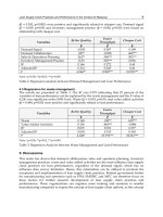
Fig. 24. The “Personal Development Space” over the Business Gateway Model
The rest of the PPS connected to in fig 24 is the reference ecosystem that a group of PPS are
parked together as is an example of Talent.net community in fig 22 that provide full
Enterprise Life Cycle (ELM) service to grow to conduct career development path. With the
features in the reference ecosystem, each individual freelancer or SME is similar staying in a
large company supporting departments such as Human Resource (Virtual Human Resource
Organization here), Procurement (Supply Chain here), Facility (such as Warehouse here),

Collaborative tools (Such as Forum, VoIP, HCT for product project management).etc.
Without proper supporting resources, individual with PPS would not be practically having

Supply Chain Management - New Perspectives
668
full coverage in learning cycle to be competitive with the one who claim up the social ladder
providing by enterprise.
Beside the administrative support in workflow collaboration, the ecosystem also act as the
coordinator to fanning in new technology such as the Dynamic Gateway Group (DGG) for
unify communication techniques, Internet of Things (IoT) for next generation sensor
network, etc in Fig 24. The ecosystem is also facilitated what the member needs in common
such as academic support from School in Supply Chain System Engineering (SCSE), and,
bargaining with the 3PL to provide logistics services for lower Logistics Level portion of the
PPS model. The distinguished design of this ecosystem is they are all adapting the same
under layer IT model and users in the ecosystem are identical in architecture except the
differentiable workflow embedded. LLL service provide who is IT compatible to the BGM
gateway is connectable between Enterprise and directly to freelancer under BGM and PPS
architecture.
10.3 Highly scalable supplier life cycle management
For large enterprise with a school of SME, freelancers they need to manage, it is always a big
challenge where it is not big enough in business transaction to justify the cost of IT
connectivity for workflow collaboration in current IT connectivity model. That is another
main reason of causing that poor result in B2B system integration in Table 1. With the IT
model and SCSE architecture in this chapter the problem can be easily resolved with the
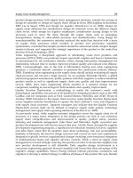
reference application in fig 25. It is a deal-mode, hybrid structure where the yellow color on
the top-right corner is still the IT setup today roughly with 20% of supplier but occupying
80% of the revenue according to the 80/20 rule.


Fig. 25. The Supplier Life Cycle Management with dual routes

In the chart, it provides a cycle to manage the new suppliers. That explains the source of IT
connectivity challenges. The 20% suppliers consume 80% of the resources and only leave the
20% for the rest. For company like Texas Instruments, ADI, or Players working in analog
industry with thousands of product lines, that is the major bottleneck of business
development and scale up when managing SME suppliers manually is an unsolvable
solution in productivity.
The left side of fig 25 applying the SCSE architecture is the suggested solution to high
product mixes industry with small qty in technological segment. The manually operating
production line can adapt the model here with appropriated LLL service provide to kick
Stable
Relationship
Fast
Switching
LLL with
Rapid
Connectivity
Ramp to
volume
20%
80%
IT
Auto
Manual
20%
Connectivity
horizon
% of
suppliers
Engineering horizon
(Industrial Specific)

N-type foundry model
ESP
Paid 2%
Resource
for Transit
Supply Chain System Engineering: Framework Transforming Value Chain
in Business Domain into Manageable Virtual Enterprise and Participatory Production
669
start the “Cover what you do best, Link to the rest” cycle in on-demand basis. Once a
supplier is growing up in volume as indicated, it reaches the criteria of entering the “N-
type” to become N+1 of the matured, IT pool. That completes the cycle seamlessly under the
IT and cost constraints. The ESP is an Engineering Service Provider it could be either
performing by internal Business Unit who responsible for the product line or hired
contractor out of the dual cycle.
10.4 Low maturity level in facility supporting participating production
The IT infrastructure in this section has covered the full spectrum of the SCSE architecture
and what it needs to connect to PPS therefore connectable to public space to complete the
connectivity all the way to nested society. This is why the research team is “accidentally”
find the redefined SCSE is the physics of the nested society when it has to resolve the SME
part of the connectivity issue to work with SME especially the world is decoupling into
smaller size of enterprise, both dominantly and globally. The IT model also demonstrates
the scalability because of the “parking” concept under the same 1+6 flow model with the
cost equation (9) and very unique feature such as “pretending” capability to allow dynamic
skin to participate virtual enterprise activities via the VHRO model. Covering full ELM cycle
and reference design in ecosystem empower individual to have equal power in IT to
compete with large enterprise. The unique segregated network design is highly simplified
the network size and complexity, hardware accelerated network provide real power of huge
network, therefore IoT reference model is doable. The research team suggests the maturity
of the current design in participatory Production is moderated after all years test and
validation. It is just time to release to “production” to have more field test where the

research team the maturity level in the field is low. Unfortunately, the study shows the
higher the N-factor of the participatory Production, the stronger dependency of the public
facility to make it success. However, it is also a bright side since it implies it is an attractive
business to players who wants this market because of the positive loop of business model:
High-N factor value chain pair with Participatory Production service provider is the
winning pair of the global competition. That is opportunity.
11. Conclusion
The Participatory Production in this chapter representing the most complicated value
network on the extreme side of private space and it has been demonstrated by peeling off
layer by layer systematically through the document hierarchy. The System Engineering
approach to conduct requirements, allocation, and deployment process is a self-explanatory,
a best-practice approach like the DoD 4245.7-M standard to delivery framework for
implementation. For enterprise, this chapter provides a rock solid path to transform into
Triple-A virtual enterprise in an ultra high degree of freedom with on-demand human
capital capability. For an individual, this chapter provides a full scalable career path from
freelancer, SME to large enterprise in a participatory manner. For SCSE, the bidirectional
pair in the 3D model determines its capability of being the physics of running a complicated
complex operation. As a solution space including both enterprise and an individual, SCSE is
nominated as the best “physics” candidate to running a nested society. On the other hand,
the SCSE is the first user-centric framework that transforms the IT-centric languages into the
operation domain languages to help an executive walking out of the mind map to make the

Supply Chain Management - New Perspectives
670
right decision himself directly not through the IT or a consultant to clear out the
accountability. Although the model in this chapter is only covering the detail in the post-
milestone C of the acquisition cycle, the maturity of the overall SCSE and the associated IT
model is sufficient as the first set of infrastructure to support the nested society to start the
iterating process of improvement. This chapter concludes that the nested society as the end
point of the IT revolution is set when the SCSE as the physics of running the nested society

is confirmed.
Another purpose of this publication is to accelerate the fusion process of the IT revolution
since the search team also suggests the review process of the academic system today is one
of the barriers that slow the fusion process. If human capital crossing 3 disciplines is a
natural barrier of any review board, it implies that any topic, paper, proposal that has more
than 3 disciplines will be naturally denied since no eligible referees can be found
adequately. Or, the topic like the physics of running the nested society, triple-A enterprise
might take decades to bubble up to the top of the hierarchical tree in the current academic
structure. That might explain why only 10% of samples in the literature research going the
multiple disciplines approach. For a super scale management solution like that, DoD
stepped out to carry out the DoD 4245.7-M standard is an good example to accelerate the
complex solution. DoD is responsible for tax money therefore accountable to the project
management to invent the standard for a defense project. But for the nested society or
Participatory Production challenges today, who should be accountable in the government
level to lead the way when the competitor of enterprise is an aggressive governor not the
war between enterprises? The game rules have changed and a new game plan is required in
the “FREE economy” campus.
12. Acknowledgments
I would like to thank the many groups that made the SCSE and KNOWLEDGE
CONTAINER hypothesis become a reality since 2003. The First is the engineering support
from the Flow Fusion Research Laboratory for their expertise, advice in the skeleton and
architecture design: Dr. Lu’s nerve network and Knowledge model; SCP system designer
Carol Wu, UCC expert Xiao Wu, system architect David Yen and many volunteers not listed
here for valuable discussions, sharing their insights, and meeting over the weekend. The
Second, is the academic support from Dr. Stracener, who brought up the System
Engineering idea to merge with the Supply Chain, and Dr. Yu, who gave all the advice on
supply chain when the fusion process is performing. The third group are the experimental
facilities such as Texas Instruments, Foxcavity, EDS, AIML, EA etc to leverage the lessons
learned from their industries. The Fourth, and not the least, is the implementation team in
Nanjing, led by Chris Chen in community technology, Lionic in hardware-accelerated

network security, ZyCoo in VoIP platform, Taohua in the collaborative set top box, and
more participatory partners to let the dream go live
13. References
Chan, L.K., S.W. Cheng and F.A. Spiring (1988) , “A New Measure of Process Capability:
Cpm,” Journal of Quality Technology, 20,162-175
Christopher, M.(1992) "Logistics and Supply chain Management", Pitman Publishing,
London
Supply Chain System Engineering: Framework Transforming Value Chain
in Business Domain into Manageable Virtual Enterprise and Participatory Production
671
Croom, S. (2000) "The Impact of Web-based Procurement on the Management of Operating
Resources Supply", Journal of Supply Chain Management; Tempe, Vol. 36, Issue 1,
pp. 413
Dertouzos, M. L. (2001) “The Unfinished Revolution: Human-Centered Computers and
What They Can Do For Us”. MIT, HarperCollins
Enslow, Beth (Aug 2006) "The Global Supply Visibility and Performance Benchmarking
Report”, Aberdeen Group
Gulati, R.(2008) , “Silo Busting: Transcending Barriers to Build High-Growth, Customer-
Centric Organization,” Evanston, Northwest University, 2007. To be published by
Harvard Business School Press in 2008
Hajime Kita, Mikihiko Mori, Takaaki Tsuji (2008), "Toward Field Informatics for
Participatory Production," Informatics Research for Development of Knowledge
Society Infrastructure, International Conference on, pp. 67-72, International
Conference on Informatics Education and Research for Knowledge-Circulating
Society.
Houlihan, J. (1974) “Supply Chain Management”. Proceedings of the 19th Int.
Tech.Conference BPICS, pp. 101‐110
Kai, Lukoff ( Sept. 2010) “Alibaba and eBay: More competition than cooperation, despite a
show of friendship”,San Francisco, VentureBeat
Jarvis, Jeff (Feb 2007). “New rule: Cover what you do best. Link to the rest”, BuzzMachine

Lamming, R.C. (1993) "Beyond Partnership: Strategies for Innovation and Lean
Supply",Prentice‐Hall,Hemel Hampsted
Lee, Hau L.(Oct. 2004), “The Triple-A Supply Chain”, HBR
Li,Wei and Cheng,Jinhua (Jul 2003) "The SMEs Development and China Economy",USA-
China Business Review(Journal), Volume 3, No.7,ISSN 1536-9048
Matthews, Julian (March 2008) “Alibaba Group - China’s E-Commerce Giant”, the
Chindians, Kuala Lumpur, the confluence of news on China and India, March 21,
2008
Merco Press (May 2011),"China became world’s top manufacturing nation, ending 110 year
US leadership", HIS Global Insight, UTC, May 14th 2011
Milesa, Raymond E. and Snow, Charles C.(March 200&), “Organization theory and supply
chain management: An evolving research perspective”, Journal of Operations
Management, Volume 25, Issue 2, Pages 459-463
Nolan,Peter; Liu, Chunhang;Zhang,Jin (2007) “The Global Business Révolution, the Cascade
Effect, and the challenges for firms from developing countries », Oxford Journal ,
Vol. 32, Issue 1, Pp. 29-47
Nolan,Peter (2008), "Capitalism and freedom: the contradictory character of globalization",
Anthem
Oscar, A., Saenz, A. and Chen, C.S. (June 2004) “Framework for Enterprise Systems
Engineering” LACCEI, Miami, FL
Pisani, Jo (March 2006) “Industry Overview-improving focus”, Pharmaceutical Outsourcing
Decisions, SPG Media Limited
Porter M. E. (1998) « Competitive Advantage CREATING AND SUSTAINING SUPERIOR
PERFORMANCE », Free Pr, ISBN: 0-684-84146-0
Raynor, William (Feb. 2003) “Globalization and the Offshore Outsourcing of White-Collar
Jobs”, Business Week

Supply Chain Management - New Perspectives
672
Rebovich, George Jr. (Nov. 2005) “Enterprise Systems Engineering Theory and Practice ,

Volume 2: Systems Thinking for the Enterprise: New and Emerging Perspectives “,
MITRE
Slack,Nigel (Dec. 1995) "Operations Strategy" (1st Edition), Prentice Hall
Slack, N., Chambers, S., Harland, C, Harrison,A. and Johnstone, R., (1995) "Operations
Management",Pitman,London
Supply Chain Operation Reference (SCOR) Model,
Tan, K.C. (2001) "A framework of supply chain management literature", European Journal of
Purchasing and Supply Management, 7(1), 39-48
Tsai P. T and Lu, T. M. (2011) “A Self-Aligned Business Gateway Model to Manage Dynamic
Value Chain and Participatory Production: Knowledge Management Prospective
to Distributed Organization”,
Tsai, T.P., Lu, M. T., and Stracener, J. (March 2011) “A Simple Knowledge Container
Skeleton to Build a Nested Society: Bridging Personal Development to
Participatory Production”, 7th International Conference on Technology,
Knowledge and Society, Bilbao, Spain
Tsai, T. P., Stracener, J., Yu, J., and Wang, F. (April 2008), « Transforming IDM into
Distributed Value Network: Framework Forming a New Branch and a Case Study
in High Precision Analog Semiconductor Industry », CSER 2008 Conference.
Tsai, T.P., Yu, J., Stracener, J. and Wang, F.C.(June 2008). Delivery quality product in value
chain: a case study to rebuild broken quality system in piecewise organization.
Proceedings of International Conference on Awareness in Product Development
and Reliability, Chengdu, China.
Tsai, T.P., Yu, J., and Stracener, J. (Dec. 2009) “BACK TO BASIC: MANAGING SUPPLY
CHAINS COLLABORATION BYCONTINUAL IMPROVEMENT IN OVER-THE-
NET OPERATION MEETING”, DET2009, Hong Kong
Tsai, T. P. and Wang, F.(2004), “Improving Supply Chain Management: A Model for
Collaborative Quality Control,” IEEE/ASMC 2004, pp. 36-42.
Tsai, T.P., Yu, J. and Yun, S. (2008), “Proactive Supply Chain planning: a Dynamic
Quantitative Planning Model,” The 3rd World Conference on Production and
Operations Management, Tokyo, Japan

Viswanathan, Nari (August 2008) “Process Collaboration in Multi-Enterprise Supply Chains
– Leveraging the Global Business Network”, Aberdeen Research
Willoughby,W. J. Jr.(1985) "DoD 4245.7-M: Transition from Development to Production",
Task Force on "Transition from Developement to Production", 1982 Defense Science
Board, published by BMP
Wu, Jeffrey (August 2008), “Economic uncertainties stimulate LCD-TV outsourcing”. iSuppli
Corp
30
The Research on Stability of Supply
Chain under Variable Delay Based
on System Dynamics
Suling Jia, Lin Wang and Chang Luo
School of Economics & Management
Beihang University
China
1. Introduction
With the swift development of modern science and network technology and fortified trend
of economics globalization, the cooperation between supply chain partners is happening
with increasing frequency and the cooperation difficulty increased correspondingly. Supply
chain is a complex system which involves multiple entities encompassing activities of
moving goods and adding value from the raw material stage to the final delivery stage.
Feedback, interaction, and time delay are inherent to many processes in a supply chain,
making it a dynamics system. Because of the dynamics and complex behaviors in the supply
chain, the study on the stability of supply chain has become an independent research field
only in last decade. At the same time, the great development of control theory and system
dynamics provides an effective way to understand and solve the complexity of evolution in
the supply chain system.
The research on stability of supply chain was put forward during the studying of bullwhip
effect. According to the paper of Holweg & Disney (2005), the development of the research
on stability of supply chain and bullwhip effect can be divided into six stages:

1. Production and Inventory Control (before 1958)
Nobel laureate Herbert Simon (1952) first suggested a PIC model based on Laplace
transform methods and differential equations. In the model, Simon used first order lag to
describe the delay of stock replenishment. Vassian (1955) built continuous time PIC model
using Z transform. Magee (1958) solved the problems of inventory management and control
in order-up-to inventory policy. At this stage, early PIC models were built based on control
theory and the dynamics characteristics of PIC systems were discussed.
2. Smoothing production (1958-1969)
In the early 1960s, Forrester (1958, 1961) built the original dynamics models of the supply
chain using DYNAMO (Dynamic Modeling) language. He revealed the counterintuitive
phenomenon of fluctuations in supply chain. The methods Jay Forrester proposed have
gradually developed into system dynamics methodology which is used to research on
dynamics characteristics of supply chain systems. For the bullwhip effect in discrete-time
supply chain systems, analytical expression of the change in inventory under order-up-to
policy was presented based on certain demand forecasting method (Deziel＆Eilon,1967). At

Supply Chain Management - New Perspectives
674
this stage, the problems such as seasonal fluctuations in inventory and demand
amplification had gained attention, but the terms “bullwhip effect” and ”stability of supply
chain” were not formally proposed, the emphasis of the academic research during this time
was the traditional production management.
3. The development of control theory (1970-1989)
Towill (1982) built a relatively complete PIC system model without considering the feedback
control loop of WIP (work in process). Bertrand (1980) studied the bullwhip effect and
inventory change in an actual production system. According to the above researches,
customer demand was assumed constant and productivity was random. Bertrand (1986)
made further study on the bullwhip effect and inventory change in PIC system with
feedback control.
4. Stage of “Beer Game” development (1989-1997)

Sterman (1989) suggested a system dynamics general stock management model after doing
experimental study on “beer game” of MIT and analyzing 2000 simulation results based on
system dynamics. Using continuous time equation, Naim＆Towill (1995) discussed the
feedback control and stock replenishment with first order lag in a supply chain model. The
“beer game” and the corresponding problems in supply chain have been studied until now,
recent research focus on information sharing and bullwhip effect in supply chain (Croson＆
Donohue, 2005). At this stage, system dynamics methodology has been deeply applied to
the field of supply chain (Towill, 1996). Both system dynamics methodology and control
theory emphasize the importance of “feedback control” to stability of supply chain, Sterman
also considered the effects of decision behavior on fluctuation of inventory and order.
5. The further development of “bullwhip effect” (1997-2000)
Lee et al. (1997a, 1997b) pointed out the clear concept of “bullwhip effect” and identified
four major causes of the bullwhip effect(demand forecast updating, order batching, price
fluctuation, rationing and shortage gaming).From then on, academic circles set off an
enthusiastic discussion centering on bullwhip effect. However, research papers during this
period didn’t make thorough study of feedback control (Holweg＆Disney, 2005).Later
studies showed that there were more than four significant bullwhip generators(Geary et
al.,2006), but the views of Lee et al. have been widely received and quoted up to the present
(Miragliotta, 2006 ).
6. The stage of avoiding bullwhip effect (after 2000)
The dynamic characteristic of supply chain represented by bullwhip effect had received
considerable attention and many researchers shifted the focus of work to prevention of
bullwhip effect at this time. Represented by Towill, Dejonckheere and Disney, a number of
scholars brought control theory deeply to the research of bullwhip effect and related
problems. They proposed APIOBPCS (Automatic Pipeline, Inventory and Order Based
Production Control System) on the basis of methods and achievements from system
dynamics (Disney＆Towill, 2002, 2003a; Dejonckheere et al., 2003; Disney el at., 2004; Disney
el at., 2006). The study on stability of supply chain has become an independent research
field at this stage and the following studies are mostly done using control theory based on
PTD (pure time delay) assumption. Up to now, the research of preventing bullwhip effect in

multi-stage supply chain system has breakthrough progress(Daganzo,2004; Ouyang＆
Daganzo, 2006).
This chapter focuses on the stability of supply chain under variable delay based on System
Dynamics methodology. First, we builds a single parameter control model of supply chain,
By simulations and related analyses, a quantitative stability criterion of supply chain system

The Research on Stability of Supply Chain under Variable Delay Based on System Dynamics
675
based on system dynamics is proposed, this criterion evaluates stability by the undulate
phenomenon and convergent speed. Then the stability characteristics in single parameter
control model with two different delay structures (first order exponential lag and pure time
delay) are discussed and the corresponding stable boundaries of the supply chain model are
confirmed. Second, based on “system dynamics general stock management model” and
control theory, the general inventory control model is built. Combined with the quantitative
stability criterion of supply chain system proposed earlier, we analyze the complexities of
the model under different delay modes. Finally we present the stable boundary and feasible
region of decision and give our conclusions. This research indicates that delay structure is a
key influencing factor of system stability.
2. Stability criterion of supply chain based on system dynamics
The differences of quantitative description of bullwhip effect result in different definitions of
stability of supply chain. Lee et al. (1997a, 1997b) described qualitative evidence of demand
amplification, or as they called it, the bullwhip effect, in a number of the retailer-distributor-
manufacturer chains and claimed that the variance of orders may be larger than that of
sales. In order to gain more insight on what is really happening, Taylor (1999) suggested
analysis on both demand data (passed from company to company) and activity data (e.g.
production orders registered within the company). The variance ratio is by far the most
widely used measure to detect the bullwhip effect. It is defined as the ratio between the
demand variance at the downstream and at the upstream stages (Miragliotta, 2006). As
variance ratio is a static index, it is difficult to describe the complex and dynamic nonlinear
system problems. In this section, we will not apply the variance ratio to measure the

stability of supply chain system.
The theories and methods in nonlinear dynamics are applied to the studies on stability and
bullwhip effect of supply chain and several criterions for describing and judging the
stability of supply chain system are formed, such as peak order amplification, peak order
rate overshot, noise bandwidth, times of demand amplification (Disney＆Towill, 2003b; Jing
Wang et al., 2004; Riddalls＆Bennett, 2001; Zhang X, 2004;). The above criterions are used on
the premise of testing the dynamic behavior of supply chain system. The test function is
usually step function, pulse function or pure sine function, not the actual demand function.
The purpose is to distinguish the effect of internal and external factors on stability of supply
chain system. Some studies based on cybernetics directly adopt the distinguish methods in
nonlinear dynamics, several methods are as following: Lyapunov exponent method; critical
chaos; state space techniques (see for example Huixin Liu et al., 2004; Lalwani et al., 2006;
Riddalls＆Bennett, 2001; Xinan Ma et al., 2005). However, these methods are applied under
a lot of constraint conditions and some parameters do not have specific economic meaning,
sometimes it is difficult to obtain ideal result, but the basic idea of analyzing structure
characteristics of the system to measure stability in cybernetics is worthy of learning.
Although the researchers have already pay attention to the problems of stability and
complexity in supply chain system, they focus on revealing dynamic characteristic of the
system and pay little attention to the problems such as stability criterion, stable boundary,
and feasible region of decision of supply chain system. Qifan Wang (1995) measured the
stability of system by analyzing open-loop gain, the method required all variables in
feedback loop to be continuous and derivable and it is not applicable to high order
nonlinear system. Sterman (1989, 2000) adopted the concept of “peak amplification” to

Supply Chain Management - New Perspectives
676
describe the dynamic characteristics of system during the research on beer game and
general stock management system, but he didn’t give a specific stability criterion.
Combining system dynamics and chaos theory, Larsen et al. (1999) described the stability of
supply chain system from a chaos perspective, but the calculation of the study is a time-

consuming and difficult task. Since now, there is no quantitative stability criterion of supply
chain systems based on system dynamics, which seriously restrict the application of system
dynamics into further research on stability of supply chain.
2.1 Single parameter stock control model of supply chain
2.1.1 Basic assumptions
The stock control model of supply chain in this section can be understood as one node along
the chain, the basic assumptions are as following:
i. The downstream demand mode is uncertain, do not make prediction on it.
ii. There is no restriction on inventory capacity.
iii. There exists delay time (DELAY) in the sending of products to downstream and the
average delay time is constant. The orders is described as WIP (work in process) before
the products arrive.
iv. There is no reverse logistics, products can’t be returned to upstream.
v. The supply chain members adjust orders according to demand from downstream and
actual storage and maintain the inventory at a desired level.
2.1.2 Structure of the model
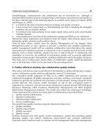
Figure 1 presents the single parameter stock control model of supply chain discussing in this
section.


Fig. 1. The single parameter stock control model of supply chain
To facilitate the model description, the following notations are introduced:
OR: the order quantity at time t,
WIP: the orders placed but not yet received at time t,
ALPHAi: the rate at which the discrepancy between actual and desired inventory levels is
eliminated, 0≤α
i
≤1,

The Research on Stability of Supply Chain under Variable Delay Based on System Dynamics

677
I*: the desired inventory level,
I: the actual inventory level at time t,
D: the actual demand at time t,
AI: the adjustment for the inventory level at time t.
Figure 1 is built on the basis of the generic stock-management model proposed by Sterman
(1989). The adjustments include two aspects: first, there exist two different delay structures
(first order exponential lag and pure time delay) in the model; second, without
consideration of WIP adjustment, the orders depend on demand and inventory adjustment.
The above adjustments simplify the feedback control loop of inventory, making the system
affected by just one negative feedback loop. Theoretical basis of the adjustment is the
analytic method of “open-loop” in system dynamics methodology (Qifan Wang, 1995;
Sterman, 2000).
The above model adopts the experimental methods to describe the individual behavior in a
common and important managerial context. It contains multiple actors, feedback,
nonlinearities, and time delay. The parameters of the order policy are estimated and the
order policy is shown to explain the decision maker’s behavior well.
2.1.3 Variable settings
As shown in figure 1, the indicated orders IO depend on demand D and adjustment for
inventory AI ，so it can be defined as the sum of D and AI. There exists the transmission
delay of orders between two successive levels and the delay mode can be represented by a
standard function DELAY of system dynamics, including first order exponential lag and
pure time delay. The desired inventory I* is constant. As products can’t be returned to
upstream, the order rate OR must be positive. That is:
IO=D+AI (1)
OR = Max (0, IO) (2)
AR = DELAY (OR, DT) (3)
Considering the stock and flow structure, the stock of WIP is the accumulation of the order
rate OR less the acquisition rate AR. Similarly, the stock of inventory I is the accumulation of
the acquisition rate less the demand D.

WIP=

[
OR
(
t
)
−AR
(
t
)
]
dt



+WIP


(4)
I=

[
AR
(
t
)
−D
(
t

)
]
dt



+I


(5)
where WIP


and I


are the initial values at time t
0
, demand D is an external variable that
can’t be controlled.
The adjustment for the inventory results in the negative feedback mechanism which
regulates the inventory. The adjustment is linear in the discrepancy between the desired
inventory and the actual inventory. That is:
AI = α
i
(I* - I) (6)

Supply Chain Management - New Perspectives
678
where α

i
is the rate at which the discrepancy between actual and desired inventory levels is
eliminated, 0≤α
i
≤1. The value of α
i
represents the sensitivity of decision-maker to the gap
between the desired inventory I* and actual inventory I. So the ordering policy can be
described as follows:
IO = D + α
i
(I* - I) (7)
The ordering policy is based on the anchoring and adjustment heuristic
(Tversky＆Kahneman, 1974). Anchoring and adjustment heuristic has been widely applied
to a wide variety of decision-making tasks in the field of control theory and system
dynamics methodology (see for example Sterman, 1989; Riddalls＆Bennett, 2002; Larsen et
al., 1999; Huixin Liu et al., 2004). From (7) we can see that without demand forecasting, the
ordering policy can be described by the single parameter α
i

2.2 Dynamic characteristics analysis of system
2.2.1 Simulation design
Suppose the system is in a stable state at the initial time without fluctuation of inventory
and order rate. When the system is disturbed by a small perturbation on demand, we can
study the system behavior from the response curve of inventory or order rate. With
reference to Sterman (1989) and Riddalls＆Bennett (2002), the initial values (unit) of
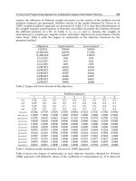
variables are presented in Table 1.The model is built using well-known system dynamics
simulation software, Vensim PLE. The run length for simulation is 60 weeks.

WIP




I*
I


DT α
i

D



300 200 200 3 1 100
Table 1. Initial values of variables
The demand pattern is a step function, that is, the demand stays at an original level up to a
certain instant and thereafter is increased to a shifted level. In this study, there is a pulse in
the demand in week number 5, increasing its value to 120 units/week.
In the simulation, the decision parameter α
i
is changed with a small decrement from 1.00 to
0.00 so as to simulate various ordering decisions. We concentrate on illustrating how minor
changes in the decision parameter can affect the dynamics and stability of the system.
System dynamics and relevant studies show that the size of step input of demand and the
desired inventory will not affect the structural stability of the system (Croson＆Donohue,
2005; Sterman, 1989, 2000).
2.2.2 Dynamics characteristics of system under first-order lag
If the delay structure of WIP is first-order lag, the (3) can be described as:


()

=


[AR(t)−0R(t)] (8)
When α
i
changes continuously, the response curves of inventory I* and desired rate OR can
always converge to the stable state, that is, I=I* and OR=D
.
Figure 2 shows two typical
patterns of behavior in the converging process: smooth convergence (α
i
=0.1) and fluctuant
convergence (α
i
=0.8). The simulation indicates that the transition between two patterns of
behavior happens when α
i
changes gradually, and when α
i
∈[0, 1], there are only the above
two typical behavior patterns.

The Research on Stability of Supply Chain under Variable Delay Based on System Dynamics
679

Fig. 2. The response curves of inventory and order rates under first-order lag (DT=3)
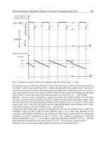
2.2.3 Dynamics characteristics of system under pure time delay

If the delay of WIP is pure time delay (PTD), then Eq. (3) can be described as:
AR (t) = OR (t - DT) (9)
With a continuous change of α
i
,

the response curves of inventory and order rate show four
kinds of behavior patterns: smooth convergence (α
i
=0.1); fluctuant convergence (α
i
=0.3);
oscillation with equi-amplitude (α
i
=0.52); divergent fluctuation (α
i
=0.58).It is worthwhile to
note that the above response curves appear to be oscillation with equi-amplitude only when
α
i
takes a special value (e.g. α
i
=0.52) and this special value is a critical point at which the
system curves begin to divergent. Figure 3 shows the response curves of inventory and
order rates under pure time delay.


Fig. 3. The response curves of inventory and order rates under pure time delay (DT=3)
2.3 Stability analysis and criteria of supply chain
2.3.1 The definition of stability

There are different definitions of stability of supply chain. The traditional ideas of system
dynamics state that only the behavior of smooth convergence is stable while the other
fluctuate behaviors are unstable (Forrester, 1958). The main reason is that system dynamics
methods focus on systems under first-order lag, and the studies on stability of supply chain
emphasize the two above situations as shown in figure 2.

Supply Chain Management - New Perspectives
680
Scholars using control theory stress the importance of pure time delay. It is commonly
accepted that fluctuant convergence is a gradual process of system to be stable and
oscillation with equi-amplitude is a critical state of stable system. Based on the definition of
stability in control theory and the methods applied by system dynamics, we propose the
following definition of stability of supply chain system:
Definition 2.1: Suppose the system is stable at the initial time, when imposing a small step
disturbance on demand, if the inventory (or order rate) can get stable at a certain
equilibrium level after a period of time, then the system is stable.
There are two points to be stressed: first, the disturbance imposed to the system can’t be too
large, as the large disturbance may destroy the structure of real system and the simulation
results can deviate from the actual situation of the system; second, the structure and
surroundings of economic system may not always keep in a specific condition, so the system
can only keep steady state within a limited period of time. In addition, computer simulation
and calculation can’t last for an indefinitely long time.
2.3.2 Stability criterion
Simulations show that for both first-order system and PTD system, when the decision
parameter α
i
change from 0.00 to 1.00, the behavior patterns of response curves of inventory
and order rate undergo a gradual change from convergence to fluctuation without any
sudden change as shown in figure 4. Therefore, we can test the stability of system from the
appearance of response curve of inventory I or order rate OR.



Fig. 4. The gradual change of response curve of inventory in two systems
The response curves shown in figure 4 can be abstracted to the general form of inventory
fluctuation as shown in figure 5. As α
i
takes different values, it is difficult to obtain the
inventory curves changing laws in the stock control model. Therefore, we can’t give a
unified description on the fluctuating behavior by analytical methods. Although inventory
fluctuation curves can well reflect dynamic behaviors of the system, it is difficult to make a
horizontal comparison among the above curves.
As the underlying cause of the fluctuation of inventory is the deviation between actual
inventory I and desired inventory I*, we use the area between the two curves to describe the
fluctuation in supply chain. This practice is similar to the method in cybernetics that use
“noise bandwidth” to make quantitative description of bullwhip effect (Dejonckheere et al.,
2003).

The Research on Stability of Supply Chain under Variable Delay Based on System Dynamics
681


Fig. 5. The general behavior pattern of inventory fluctuation
As shown in figure 5, assuming that the inventory curve begins to fluctuate at time t
0
, the
inventory curve and desired inventory level intersect at time t
1
, t
2
…t

i
…t
n
in succession, and
the area between two curves can be divided into several parts S
1
，S
2
…S
i
S
n
. Let the
absolute value of the area between the two curves be s
n
，that is:
s
n=
∑|
S

|



(10)
i. If the system is smooth convergence, then there is only one arc between the two curves:
s
n
= |S

1
| (11)
ii. If the system is fluctuant convergence, then |S
i
| > |S
i+1
| (i=1,2…n). There exists a
natural number N, when t ≥ t
N,
I ≡ I*,|S
N+1
| ≈ 0, and:
lim
→
s

=s

=
∑|
S

|
=C


(Constant) (12)
iii. If the system is oscillation with equi-amplitude, then |S
1
|=|S

2
|=…=|S
i
| =…=|S
n
|,
and:
s
n
=
∑|
S

|
=n
|
S

|


(13)
iv. If the system is divergent fluctuation, then |S
i
| < |S
i+1
| (i=1,2…n) and:
lim
→
s


=∞ (14)
To sum up, that is:


|
I
(
t
)
−I
∗
|
dt=
∑|
S

|
=s







(15)
S
(
t


)
=

|
I
(
t
)
−I
∗
|
dt




(16)
where S is the inventory integral curve. We can distinguish the behavior of the system
according to the form of curve S, that is, S curve can be used as the stability criterion of the
system.

Supply Chain Management - New Perspectives
682
The S curve can be obtained by the software, Vensim PLE. As shown in figure 6, we present
the S curves of PTD system with different decision parameter α
i
corresponding to figure 3(a)
and the trend of S curve is the same as stated before. When S curve keeps a horizontal state
or small-scope fluctuation around the horizontal line finally (e.g. α

i
=0.1; 0.3), the system has
returned the stable state. That is, the order meet the demand completely and I=I*.
According to the definition of stability and the above simulation analysis, the sufficient
condition of the system to be stable is presented as following:
lim
→
S(t)=C (Constant) (17)
Eq. (17) can be replaced by the following description:
Definition 2.2: Assuming t
0
is the starting time of simulation and t
F
is the end time of
simulation, if there exists t
s
(t
0
≤t
s
≤t
F
) to make S(t) = C (Constant), then the system is stable.
The constant C can be understood as the system stable level, and the smaller the value of C,
the better stability of the system. In the condition of step disturbances on demand and no
prediction, C is positive.






Fig. 6. Inventory integral curve under pure time delay (DT=3)
The value of S (t
n
) directly reflects the deviate degree of the actual inventory I from the
desired inventory I*. When the inventory is too high or too low, the holding cost and
shortage cost will increase accordingly. Therefore, the S curve can intuitively measure the
potential cost burden. On the other hand, the S curve reflects not only the general situation
of system behavior but also the behavior change with time varying. Compared to stock
variance, the S curve can measure the consequences of long time small-scope fluctuation
(with small stock variance) of the system.
In conclusion, the S curve is able to reflect different behavior patterns in supply chain
system. What’s more, it is more convenient and visible to estimate the effect of fluctuation
on inventory cost, ordering policy and forecasting. Besides, according to the definition of
stability, the two behavior patterns of first-order system reflect that such systems are always
stable, and this conclusion is in agreement with the results obtained from cybernetic
methods. The relationship between typical behavior patterns and stability criterion is
summarized as shown in table 2.

The Research on Stability of Supply Chain under Variable Delay Based on System Dynamics
683

Inventory status Sharp of S curve Delay mode System state
Smooth convergence
Be similar to exponential curve,
base number∈(0 1)
First-order;
PTD
Stable
Fluctuant convergence

Be similar to exponential curve,
base number∈(0 1)
First-order;
PTD
Stable
Oscillation with equi-
amplitude
Be similar to straight line PTD Critical stable
Divergent fluctuation
Be similar to exponential curve,
Base number∈(1,+∞)
PTD Unstable
Table 2. Behavior pattern and its stability
3. Study on the stability of general inventory control system
In the last section, the dynamic characteristics of single parameter stock control system were
discussed and we adopt the inventory integral curve as the criterion for stability judgment.
Based on cybernetic studies, the dynamic behavior patterns of inventory in supply chain
system are limited to the four typical behavior patterns shown in table 2 (Lalwani et al.,
2006). Therefore, as a result of primary judge, the stability criterion proposed in the previous
section is still valid for more complicated systems.
However, the single parameter stock control model has ignored the management of WIP
and there is significant difference between theoretical model and managerial practice.
Meanwhile, the previous simulation shows that the delay structure of WIP is a key factor of
system stability. Therefore, it is of great theoretical and practical importance to study the
effect of WIP on stability of supply chain system.
In this section, based on the generic stock-management model (Riddalls＆Bennett, 2002;
Sterman, 1989), we add the WIP control loop to the previous model and built a general
inventory control system with dual-loop and double decision parameters. Then the
applicability of stability criterion is validated and the stability characteristics in double
parameters control model with two different delay structures are discussed.

3.1 General inventory control system model
3.1.1 Basic assumptions
The general inventory control system model in this section can be still understood as one
node along the chain, the basic assumptions are the same as i-iv described in 2.1.1.
Considering the management of WIP, assumption v in 2.1.1 is changed as following:
v.The supply chain members adjust orders according to demand from downstream, actual
storage and WIP, and maintain the inventory at a desired level.
3.1.2 Structure of the model
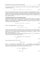
Figure 7 represents the general inventory control model:
Compared to the model in figure 1, there are three increasing variables:
WIP* the desired WIP,
AWIP the adjustment for WIP,
ALPHAwip (α
WIP
) the rate at which the discrepancy between actual and desired WIP
levels is eliminated, 0≤α
WIP
≤1,

Supply Chain Management - New Perspectives
684


Fig. 7. The general inventory control model
3.1.3 Variable settings
Except the indicated orders, the settings of other variables in inventory control loop are the
same as Eq. (2)-(6). To regulate WIP, a negative feedback mechanism is used. Adjustments
are then made to correct discrepancies between the desired and actual inventory AI, and
between the desired and actual WIP AWIP. Eq. (1) is adjusted as follows:
IO = D + AI + AWIP (18)

Since WIP* is proportional to the demand as well as the delay time, we define the desired
WIP as the delay time multiplied by the demand D. That is
WIP* = D×DT (19)
AWIP=α
WIP
(WIP*-WIP) (20)
WIP* reflects the excepted value of future delivery situation. For production-oriented
enterprises, WIP* reflects the supply capacity of upstream raw materials and production
capacity on the node; for distribution firms, WIP* reflects the channel capacity between two
nodes. In fact, there are multiple ways to measure WIP* and Eq. (19) adopts the linear
approximation method. As this chapter focuses on structure factors, when imposing small
disturbance on the system, the estimate precision of WIP* has little influence on the system
stability.
According to Eq. (6) and Eq. (20), the ordering policy is defined below:
IO = D + α
i
(I* - I) + α
WIP
(WIP* - WIP) (21)
This ordering policy is still based on the anchoring and adjustment heuristic. Compared to
Eq. (7), Eq. (21) considers two anchoring points, that is, I* and WIP*. The ordering policy is
one of the dual parameter decision rules. When α
WIP
=0, figure 6 is equivalent to figure 1.
Therefore, the general inventory control model covers the single parameter stock control
model.

The Research on Stability of Supply Chain under Variable Delay Based on System Dynamics
685
3.2 Dynamic characteristics analysis of system

3.2.1 Simulation design
Except the parameters involved in WIP, the initial values of the variables are the same as
presented in 2.2.1. For the convenience of comparison, we set the value of α
WIP
to zero, that
is, the initial state of the model is equivalent to single parameter stock control model.
We still adopt the small disturbance for stability examination, and the demand function is
unchanged:
D = D


(1+STEP (0.2, 5)) (22)
In the presence of small disturbance, the decision parameter α
i
is changed from 1 to 0 with a
small decrement Δi. At the same time, α
WIP
varies from 0 to 1 with another small increment
ΔWIP, the smaller the values of Δi and ΔWIP, the higher the simulation accuracy. The
process can be described by pseudo-code below:
For (α
i
=1; α
i
≥0; α
i
=α
i
-Δi)
{ for (α

WIP
=0; α
WIP
≤1; α
WIP
=α
WIP
+ΔWIP)
{ Run Model }
}
This section focuses on the interaction of dual-loop and verifying the applicability of
stability criterion proposed in the previous section to general inventory control system.
Through simulation, we can observe the behavior patterns of general inventory control
system and test the system stability in the situation of complete rationality (α
i,
α
WIP
∈[0,1]),
then the simulation results can be compared with that of single parameter stock control
model.
3.2.2 Dynamics characteristics of system
1. First-order system
The first-order lag is described as Eq. (8).
If α
WIP
=0, the general inventory control model is equivalent to single parameter stock
control model. From the previous analysis, when α
i
changes continuously, the response
curves of inventory I* and desired rate OR can always converge to a stable state. There are

only two typical behavior patterns: smooth convergence and fluctuant convergence.
If α
WIP
≠0, when α
i
takes a particular value andα
WIP
varies from 0 to 1 with a small increment
ΔWIP, the shapes of response curves of inventory I* and desired rate OR are still restricted
to the above mentioned two typical behavior patterns. The nearer α
WIP
approaches 1, the
more obvious the smoothness of response curves will be. The nearer α
WIP
approaches 0, the
more obvious the fluctuation characteristics of response curves will be. Figure 8 shows the
response curves of inventory of the general inventory control system under first-order lag
when DT=3 and α
i
=0.4.
Together with figure 2, it leads to the conclusion that the general inventory control system
under first-order lag is usually stable, but α
WIP
and α
i
have exerted totally different influence
on the dynamics characteristics of system. This conclusion also hold in the case when delay

Supply Chain Management - New Perspectives
686

time DT takes different values. Therefore, after preliminary analysis, WIP control loop has
weakened the fluctuation characteristics of first-order system. The greater the value of α
WIP
,
the weakening more obvious.


Fig. 8. The response curve of inventory under first-order lag
2. PTD system
The pure time delay is described as Eq. (9).
If α
WIP
=0, the response curves of inventory and desired rate will not always converge to
stable state with a continuous change of α
i
and there are four kinds of behavior patterns:
smooth convergence; fluctuant convergence; oscillation with equi-amplitude; divergent
fluctuation. Therefore, the system exhibits critical stable state and stable boundary.
If α
WIP
≠0, when α
i
takes a particular value andα
WIP
varies from 0 to 1 with a small increment
ΔWIP, the shapes of response curves of inventory I* and desired rate OR are still restricted
to the above mentioned four typical behavior patterns. Figure 9 shows the response curves
of inventory of the general inventory control system under pure time delay when DT=3 and
α
i

=0.58.


Fig. 9. The response curve of inventory under pure time delay
Although single parameter stock control model exhibits divergent behavior when α
i
=0.58,
the general inventory control system model with double decision parameters can have
convergent behavior as the value of α
WIP
increases. Together with the response curves in
figure 3, it is concluded that the general inventory control system under pure time delay is
not always stable, and the parameters α
WIP
and α
i
show entirely opposite effects on the
dynamics characteristics of system. For certain single parameter systems that are unstable,

The Research on Stability of Supply Chain under Variable Delay Based on System Dynamics
687
by adding decision parameter α
WIP
and enhancing WIP control loop, the systems can reach
stable state. Thus, WIP control loop has also weakened the fluctuation characteristics of PTD
system.
3.3 Stability analysis of general inventory control system
3.3.1 Stability criterion
Following definition 2.1, the inventory integral curve is used as the stability criterion of
supply chain system. This stability criterion can be generalized to the general inventory

control system model with double decision parameters only when the following conditions
are satisfied:
First, the response curve of inventory I (or order rate OR) is limited to the range listed in
table 2;
Second, the response curve of inventory I (or order rate OR) is gradually changing as the
decision parameters α
WIP
and α
i
change, and there is no mutation in this process.
As the WIP control loop has in fact weakened the fluctuation characteristics of single
parameter system model, the behavior patterns of general inventory control model will not
go beyond that of single parameter stock control model. Therefore, the behavior patterns of
system listed in table 2 still apply to general inventory control system model.
Figure 10 shows the traverse of the response curve of inventory under different delay
modes. Through the analysis of figure 4, figure 8 and figure9, the increased α
i
will increase
the fluctuation while the increased α
WIP
will cushion the fluctuation both in first-order
system and PTD system after disturbed, and the processes are smooth. Together with figure
10, the system hasn’t appeared other new behavior patterns and mutation points.


Fig. 10. The traverse graph of inventory curves of general inventory control system model
In conclusion, the dynamic patterns and stability criterion obtained from the analysis of
single parameter stock control system model still hold in the general inventory control
system model under first-order lag and pure time delay.
3.3.2 Stability of first-order system

This research indicates that the first-order system is always stable and the two decision
parameters have different effects on system stability. Figure 8 shows that the system
stability is increasing with the increase of α
WIP
. Similarly, we obtain the S curve of the
general inventory control system model under first-order lag (see figure 11). According to

Supply Chain Management - New Perspectives
688
definition 2.2, the constant C represents the stable level of system. Figure 11 shows that the
value of C will decrease when increasing α
WIP
under the condition of the given delay time
and α
i
. But there exists a minimum C*, when the system achieves C*, increase of α
WIP
won’t
help improve system stability. Let C* be the minimal stable level which is determined by α
i

with a given DT, α
WIP,
then determines whether the system can achieve the stable level C* or
not. Before the system achieves the stable level C*, the response curve of inventory appears
to be fluctuant convergence, but when the system has achieved the stable level C*, the
response curve of inventory tends to be smooth convergence, and the increase of α
WIP
can
only reduce the deviation between actual inventory I and desired inventory I* and postpone

the stabilizing time of the system.


Fig. 11. Inventory integral curve of general inventory control model under first-order lag
Further analysis indicates that there is an exclusive α
WIP
corresponding to α
i
(α
i
, α
WIP
∈[0,1])
to make the system achieve the stable level C*. Based on the analysis, the minimal stability
boundary of general inventory control model under first-order lag with different DT is
obtained as shown in figure 12 (x-axis is α
i
, y-axis is α
WIP
). We use S* curve to express the
minimal stability boundary, each point on the curve can guarantee that the system will
achieve the stable level C*.As shown in figure 12, the index of S* represents the value of DT.


Fig. 12. The minimal stability boundaries of first-order system under different DT

The Research on Stability of Supply Chain under Variable Delay Based on System Dynamics
689
The adjusting parameters (α
i

, α
WIP
) in the lower right region of S* curve will cause the
response curve of inventory to be fluctuant convergence while the parameters in the upper
left region guarantee the curve to be smooth convergence. The traditional views of system
dynamics consider that fluctuant convergence is unstable and only smooth convergence is
stable. Therefore, the lower right region of S* curve is the unstable region in the traditional
sense. Nonetheless, the actual decisions are influenced by many subjective and objective
factors, and the adjusting parameters (α
i
, α
WIP
) may not be the point in the S* curve.
When DT≥1, S* curve is nonlinear, otherwise, S* curve is approximate linear and all S*
curves are in the lower right region of an oblique line (α
i
=α
WIP
). In conclusion, there exists
the adjusting parameters (α
i
, α
WIP
) that make the first-order system achieve the stable level
C* only when α
WIP
≤α
i
. As α
i

and α
WIP
reflect the attitude of decision-maker on the
differences, that is, (I* - I) and (WIP* - WIP), the condition that α
WIP
is less than or equal to α
i
represents the rational choice of decision-maker. In other words, most decision-makers think
that the actual inventory is more important than WIP and they pay more attention to the
difference between the actual inventory and the desired inventory.
Since all the adjusting parameters (α
i
, α
WIP
) that make the first-order system achieve the
stable level C* exist in the lower right region of the oblique line (α
i
=α
WIP
), α
WIP
≤α
i
is a
necessary condition for first-order system to achieve the minimal stable level and this
condition is determined by the structure of first-order system itself. Whether the system can
achieve the minimal stable level or not depends on the subjective judgment of the decision-
maker and the external and internal factors. Let the oblique line (α
i
=α

WIP
) be the
conservative stability boundary and the condition that α
WIP
is less than or equal to α
i
be the
conservative stability condition. As the conservative stability condition is the result of
rational choice, the oblique line (α
i
=α
WIP
) can also be called rational stability boundary.
3.3.3 Stability of PTD system
It is known that the PTD system is not always stable and the parameters α
WIP
and α
i
show
opposite effects on the dynamics characteristics of system. Like the single parameter stock
control system model under pure time delay, we can obtain the critical stable points
(α


,α


) of general inventory control system under pure time delay by finding the critical
stable state of inventory curve with a given DT. Therefore, the critical stable condition of
general inventory control system under pure time delay is defined as following:

Definition 3.1: Suppose the general inventory control system under pure time delay is stable
at the initial time. With a given DT, when imposing a small step disturbance on demand, if
there exists the decision parameters (α


,α


) that can keep the inventory curve to be
oscillation with equi-amplitude, then the state is called critical stable state, and (α


,α


) is
the critical stable point of the system under the given DT.
Unlike the single parameter stock control system model, the critical point (α


,α


) of the
general inventory control system model is not unique. Through the traversal simulation of
α
i
and α
WIP
under certain DT, several critical stable points are found. After connecting these

points in the plane that takes α
i
as horizontal axis and α
WIP
as vertical axis, we obtain the
stability boundary of PTD system named s curve. Figure 13 shows some s curves under
different DT and the index of s represents the value of DT.
Furthermore, s curve is approximate to linear property and the lower right of s curve is the
unstable region. That is, the points (α
i
, α
WIP
) in the lower right of s curves will lead the
inventory curve into divergent fluctuation, and the points in the upper left of s curves will

Supply Chain Management - New Perspectives
690
make the inventory curve convergent. As DT increases, s curve tends to converge toward
the oblique line: α
WIP
=α
i
/2. Simulations show that the oblique line (α
WIP
=α
i
/2) is the upper
bound when s curve moves up to top left with DT increasing. Thus, it can be concluded that
the upper left area of oblique line (α
WIP

=α
i
/2) is the stable region which is independent of
delay (IoD), and the oblique line (α
WIP
=α
i
/2) is defined as IoD stability boundary of PTD
system. Since the models of supply chain in this research take no account of predictions, the
conclusions above not only validate the results obtained by cybernetic method from the
point of view of system dynamics, but also prove that IoD stability boundary is only
determined by systemic structure.


Fig. 13. The stability boundaries of PTD system under different DT
Meanwhile, there also exists a minimal stability boundary of PTD system under the given
DT. The minimal stability boundaries of PTD system under different DT are shown in figure
13. The simulation results show that the greater the DT value, the more obvious the linearity
of s* curve, when DT≥9, s* curve and the oblique line (α
WIP
=α
i
) nearly coincide. Similarly,
α
WIP
≤α
i
is also the necessary condition for PTD system to achieve the minimal stable level
and the oblique line (α
i

=α
WIP
) is the conservative stability boundary or rational stability
boundary of PTD system.
3.3.4 Discussion
The main difference between the general inventory control model and the single parameter
stock control model are the WIP control loop and the ordering strategy. The single
parameter decision rule is marked IO
1
and the two-parameter decision rule is marked IO
2
,
that is:
IO
1
= D + α
i
(I* - I) (22)
IO
2
= D + α
i
(I* - I) + α
WIP
(WIP* - WIP) (23)
As compared with Eq. (22), Eq. (23) contains the new WIP adjustment. From the static
perspective, IO
2
is greater than or equal to IO
1

under the same initial conditions and the
demand will be enlarged. But through the dynamic methods, it is found that the two-

The Research on Stability of Supply Chain under Variable Delay Based on System Dynamics
691
parameter decision rule actually restraints the demand amplification and reduces the
fluctuation of inventory and order rate because of the WIP control loop. Some studies on
stability of supply chain based on dynamic methods suggest that the increase in α
WIP
and
decrease in α
i
can contribute to improving the stability of the system (Disney et al., 2004;
Riddalls et al., 2000; Sterman, 1989), but the findings of this section indicate that the above
policies are effective only in the lower right region of the minimal stability boundary s*
curve.
Second, neither first-order system nor PTD system has the same rational stability boundary.
This rational boundary conforms well to the results of beer game (Sterman, 1989). Although
Sterman adopted first-order lag as the delay mode when modeling the beer game, the
participants hadn’t known the delay mode and they didn’t estimate the delay mode of WIP
control loop. Therefore, the conservative stability boundary or rational stability boundary
actually has nothing to do with delay.
Finally, the minimal stable level C* proposed in this section is relevant to the convergence
properties of inventory fluctuation, it can’t guarantee the minimum cost. From the point of
view of cost optimizing, there also exists an optimal boundary which depends on the ability
of inventory management and the composition of inventory cost.
4. Conclusions
To conduct quantitative analysis on the stability of supply chain system with Order-Up-To
(OUT) policy, we first built the single parameter stock control model of supply chain. By
simulation analysis, a system-dynamics-based criterion for stability judgment is proposed.

With simulation, the criterion can be used to describe the nonlinearities of supply chain
system with 1st order exponential lag and pure time delay (PTD).The criterion can also be
used to judge the influences exerted on supply chain stability by decision behavior. The
simulation demonstrates two different results. Firstly, the 1st order system is usually stable,
but there is fork effect as decision parameter changes. Secondly, there is a critical stable
bound in PTD system, which determines the feasible filed of decision.
Then a general inventory control system model is proposed. The model is provided with
two typical delay modes: fist-order exponential delay and pure time delay. According to the
concept of stability and stability criterion proposed in the previous section, stability borders
with different meanings are confirmed, which integrate the results derived from different
research methods. It is concluded that the stability of inventory control system is mainly
decided by the features of feedback systems, the subjective decision and environment take
their effects based on the feedback systems, and information sharing is propitious to
increase the stability and weaken bullwhip effect of supply chain system.
This research adopts the method of system dynamics and takes the delay modes as key
point to discuss stability of supply chain system. Although preliminary achievements have
been made, further research needs to be done on the stability of supply chain. With the
development of research, we wish this chapter will contribute to supply chain management
theories and practices.
5. References
Bertrand, J.W.M. (1980). Analysis of a production-inventory control system for a diffusion
department. International Journal of System Science, Vol.11, No.5, pp. 589-606.