Adaptive Filtering Applications Part 12 pptx
Bạn đang xem bản rút gọn của tài liệu. Xem và tải ngay bản đầy đủ của tài liệu tại đây (1.88 MB, 30 trang )
Adaptive Filtering Applications
322
PATH
FILTER
NAME
AVG.
ERROR
MAX
ERROR
RSSI
FILTER
LQI
FILTER
FUSION
FILTER
BOTH FILTER
1
Non filter 1.2750 4.0577
Avg.
RDC.
of
Avg.
Error
33%
Avg.
RDC.
of
Avg.
Error
50%
Avg.
RDC.
of
Avg.
Error
41%
Avg.
RDC.
of
Avg.
Error
49%
Avg.
RDC.
of
Avg.
Error
49%
Avg.
RDC.
of
Avg.
Error
62%
Avg.
RDC.
of
Avg.
Error
56%
Avg.
RDC.
of
Avg.
Error
68%
RSSI
Filter
1.0911 3.1117
LQI
Filter
1.0962 2.7127
Fusion
Filter
1.2807 3.0742
BOTH
filter
1.0959 2.6453
2
Non filter 3.0142 15.183
RSSI
Filter
1.0943 5.4847
LQI
Filter
1.0040 3.4574
Fusion
Filter
0.8408 3.3281
BOTH
filter
0.6495 1.8214
3
Non filter 5.3016 21.183
RSSI
Filter
2.3972 7.2861
LQI
Filter
3.0213 13.609
Fusion
Filter
1.3088 3.1259
BOTH
filter
1.3174 3.8351
Table 3. Error reduction comparison of RSSI filter, Fusion filter, proposed LQI filter and
BOTH filter
such beneficial technology. The security measures to provide Confidentiality and Integrity
have been taken into account in the design of such technology. This chapter investigates the
use of RF location systems for indoor domestic applications. Based on the assumption, low
cost and minimal infrastructure are important for consumers, the concept of RF location
system for Integrated In-door Location Using RSSI and LQI provided by ZigBee module is
introduced.
This chapter addresses the problem of tracking an object. This chapter discuss about how to
overcome the problems in the existing methods calculating the distance in indoor
environment. This chapter has presented a new Mathematical Method for reducing the error
in the location identification due to interference within the infrastructure based sensor
Adaptive Filtering for Indoor Localization using ZIGBEE RSSI and LQI Measurement
323
network. The proposed Mathematical Method calculates the distance using LQI and RSSI
predicted based on the previously measured values. The calculated distance corrects the
error induced by interference. The experimental results show that the proposed
Mathematical Method can reduce the average error around 25%, and it is always better than
the other existing interference avoidance algorithms. This technique has been found to work
well in instances modeled on real world usage and thereby minimizing the effect of the
error and hope that the findings in this chapter will be helpful for design and
implementation of object tracking system in indoor environment.
7. Acknowledgements
This work is financially supported by Korea Minister of Ministry of Land, Transport and
Maritime Affairs (MLTM) as U-City Master’s and Doctoral Course Grant Program. And
special thanks to Yen Sethia for her kind cooperation.
8. References
[1] IEEE Standard for Information Technology. (October 2003). Wireless Medium Access
Control (MAC) and Physical Layer (PHY) Specifications for Low-Rate Wireless
Personal Area Networks (LR-WPANs), Local and Metropolitan Area Networks,
Part 15.4
[2] Kamran, J. (January 2005). ZigBee Suitability for Wireless Sensor Networks in Logistic
Telemetry Applications. Master’s Thesis in Electrical Engineering, School of
Information Science, Computer and Electrical Engineering, Halmstad University,
Sweden
[3] Liu, H.; Darabi, H.; Banarjee, P. & Liu, J. (2007). Survey of Wireless Indoor Positioning
Techniques and Systems. IEEE Transactions on Systems, Man, and Cybernetics-Part C:
Applications and Reviews, Vol.37, No.6, (2007), pp. 1067-1080
[4] Tae Young, C. (December 2007). A Study on In-door Positioning Method Using RSSI
Value in IEEE 802.15.4 WPAN. Master’s Thesis in School of Electronical
Engineering & Computer Science, Kyungpook National University, Korea
[5]
[6] Dragos, N. & Badri, N. (April 2001). Ad-hoc Positioning System, Technical Report DCS-
TR-435, Rutgers University, also in Symposium on Ad-Hoc Wireless Networks,
pp. 2926-2931, San Antonio, Texas, USA, November 2001
[7] Lorincz, K. & Welsh, M. (2005). Motetrack: A Robust, Decentralized Aproachto RF-based
Location Tracking, Proceedings of the International Workshop on Location- and Context-
Awareness (LoCA ’05), Munich, Germany, May 12-13, 2005
[8] Vehbi Cagri, G. (August 2007). Real-Time and Reliable Communication Inwireless Sensor
and Actor Networks. PhD Thesis in School of Electrical and Computer Engineering,
Georgia Institute of Technology, USA
[9] Zhang, J.; Yan, T.; Stankovic, J. & Son, S. (2005). Thunder: A Practical Acoustic
Localization Scheme for Outdoor Wireless Sensor Networks. Technical Report CS-
2005-13, Department of Computer Science, University of Virginia, USA
[10] Priyantha, N.; Chakraborty, A. & Balakrishnan, H. (2000). The Cricket Location-Support
System, Proceedings of the 6
th
Annual International Conference on Mobile Computing and
Networking, pp. 32–43, Boston, MA, USA, August 6-11, 2000
Adaptive Filtering Applications
324
[11] Alippi, C. & Vanini, G. (2005). A RF Map-based Localization Algorithm for Indoor
Environments, Proceedings of the IEEE International Symposium on Circuits and
Systems, pp. 652-655, Kobe, Japan, May 23-26, 2005
[12] Bahl, P. & Padmanabhan, V. RADAR: An In-building RF-based User Location and
Tracking System. INFOCOM, Vol.2, pp. 775–784, Tel Aviv, Israel
[13] Kumar, S. (February 2006). Sensor System for Positioning and Identification in
Ubiquitous Computing. Final Thesis
[14] Bulusu, N.; Heidemann, J. & Estrin, D. (2000). GPS-less Low Cost Outdoor Localization
for Very Small Devices, Personal Communications Magazine, Vol.7, No.5, pp. 28-
34, Octobar 2000
[15] Kaemarungsi, K. (2005). Design of Indoor Positioning System Based on Location
Fingerprint Technique. Master’s thesis, University of Pittsburgh, USA
[16]
[17] CC2430 datasheet. Available from
[18] Want, R.; Hopper, A.; Falcao, V. & Gibbons, J. The Active Badge Location System.
Technical Report 92.1, Olivetti Research Limited (ORL), ORL, 24a Trumpington
Street, Cambridge CB2 1QA, UK
[19] Krohn, A.; Beigl, M.; Hazas, M.; Gellersen, H. & Schmidt, A. (2005). Using Fine-grained
Infrared Positioning to Support the Surface Based Activities of Mobile Users, Fifth
International Workshop on Smart Appliances and Wearable Computing (IWSAWC),
Columbus, Ohio, USA, June 10, 2005
[20]
[21] Fukuju, Y.; Minami, M.; Morikawa, H. & Aoyama, T. (2003). Dolphin: An Autonomous
Indoor Positioning System in Ubiquitous Computing Environment, IEEE Workshop
on Software Technologies for Future Embedded Systems (WSTFES2003), pp. 53–56,
Hakodate, Hokkaido, Japan, May 2003
[22] Priyantha, N.; Miu, A.; Balakrishnan, H. & Teller, S. (2001). The Cricket Compass for
Context-aware Mobile Applications, Proceedings of the 7
th
Annual International
Conference on Mobile Computing and Networking, pp. 1–14, Rome, Italy, July 16-21,
2001
[23] Bahl, P.; Padmanabhan, V. & Balacgandran, A. (2000). Enhancements to the RADAR
User Location and Tracking System. Microsoft Research Technical Report, February
2000.
[24] Getting, I. The Global Positioning System. IEEE Spectrum, Vol.30, No.12, (December
1993), pp. 36– 47,
[25] Simon, H. (1984). Introduction to Adaptive Filters, ISBN 0029494605, Collier Macmillan
Publishers, London
[26] Sayed, A. (2003). Fundamentals of Adaptive Filtering, ISBN 0471461261, IEEE Press Wiley-
Interscience, New York
[27] Halder, S. J.; Choi, T.; Park, J.; Kang, S.; Park, S. & Park, J. (2008). Enhanced Ranging
Using Adaptive Filter of ZIGBEE RSSI and LQI Measurement, Proceedings of The
10th International Conference on Information Integration and Web-based Applications &
Services (iiWAS2008), pp. 367-373, Linz, Austria, November 24-26, 2008
[28] Halder, S. J.; Choi, T.; Park, J.; Kang, S.; Yun, S. & Park, J. (2008). On-line Ranging for
Mobile Objects Using ZIGBEE RSSI Measurement. Proceedings of The 3rd
International Conference on Pervasive Computing and Applications (ICPCA2008), pp.
662-666, Alexandria, Egypt, October 06-08, 2008
Part 4
Other Applications
15
Adaptive Filters for Processing
Water Level Data
Natasa Reljin
1
, Dragoljub Pokrajac
1
and Michael Reiter
2
1
Delaware State University,
2
Bethune-Cookman University
USA
1. Introduction
Salt marshes are composed of various habitats contributing to high levels of habitat diversity
and increased productivity (Kennish, 2002; Zharikov et al., 2005), making them among the
most productive ecosystems on the Earth. The salt marsh consists of a halophytic vegetation
community growing near saline waters (Mitsch & Gosselink, 2000) characterized by grasses,
herbs, and low shrubs (Adam, 2002). Salt marshes exist between the upper limit of the high
tide and the lower limit of the mean high water tide (Adam, 2002). They represent an
important factor in the support of surrounding food chains, and due to the high level of
productivity their economic and aesthetic value is increasing (Delaware Department of
Natural Resources and Environmental Control, 2002; Zharikov et al. 2005). The survival and
reproduction of many species of commercial fish and shellfish is dependent upon salt marshes
(Zharikov & Skilleter, 2004). In addition, salt marshes provide critical habitat and food supply
to crustaceans (Zharikov et al., 2005) and shorebirds (Potter et al., 1991). They are often
considered as a primary indicator of the ecosystem health (Zhang et al., 1997). Because of their
ability to transfer and store nutrients, salt marshes are an important factor in the maintenance
and improvement of water quality (Delaware Department of Natural Resources and
Environmental Control, 2002; Zhang et al., 1997). In addition, they provide significant
economic value as a cost-effective means of flood and erosion control (Delaware Department
of Natural Resources and Environmental Control, 2002; Morris et al., 2004). This economic
value makes coastal systems the site of elevated human activity (Kennish, 2002).
Determining the effects of sea level rise on tidal marsh systems is currently a very popular
research area (Temmerman et al., 2004). While average sea level has increased 10-25 cm in
the past century (Kennish, 2002), the Atlantic coast has experienced a sea level rise of 30 cm
(Hull & Titus, 1986). Local relative sea level has risen an average rate of 0.12 cm yr
-1
in the
past 2000 years, but at Breakwater Harbor in Lewes, DE sea level is rising at the average rate
of 0.33 cm yr
-1
, nearly three times that rate (Kraft et al., 1992). According to the National
Academy of Sciences and the Environmental Protection Agency, sea level rise within the
next century could increase 60 cm to 150 cm (Hull & Titus, 1986).
The changes in sea level rise are particularly affecting tidal marshes, since they are located
between the sea and the terrestrial edge (Adam, 2002; Temmerman et al., 2004). The prediction
is that sea level rise will have the most negative effect on marshes in the areas where the
landward migration of the marsh is restricted by dams and levees (Rooth & Stevenson, 2000).
Adaptive Filtering Applications
328
If sea level rises the almost certain prediction of 0.5 m by 2100 and marsh migration is
prevented, then more than 10,360 km
2
of wetlands will be lost (Kraft et al., 1992). If the sea
level rises 1 m then 16,682 km
2
of coastal marsh will be lost, which is approximately 65% of all
extant coastal marshes and swamps in the United States (Kraft et al., 1992).
Due to an imminent potential threat which can jeopardize the Mid-Atlantic salt marshes, it
is very important to examine the effect of sea level rise on these marshes. The marshes of the
St. Jones River near Dover, DE, can be considered to be typical Mid-Atlantic marshes. These
marshes are located in developing watersheds characterized by dams, ponds, agricultural
lands, and increasing urbanization, providing an ideal location for studying the impacts of
sea level rise on salt marsh extent and location. In order to determine the effect of sea level
rise on the salt marshes of the St. Jones River, the change in salt marsh composition was
quantified. Unfortunately, as for most marsh locations along the Atlantic seaboard, the data
on sea level rise for this area was not available for comparison with marsh condition.
However, a wide data set for this area is available through a water quality monitoring
program, and if it could be properly processed and analyzed it could result in sea level rise
data for the location of the interest.
In this chapter, we describe the application of signal processing on the water level data from
the St. Jones River watershed. The emphasis is on adaptive filtering in order to remove the
influence of upstream water level on the downstream levels.
2. Data
The St. Jones River, in central Delaware, is 22.3 km long (Pokrajac et al., 2007a). It has an
average mean high water depth (MHW) of 4 m in the main stem, and an average width of
15 feet. The site’s watershed area is 19,778 ha, and the tidal reaches are influenced by fresh
water runoff from the urbanized area upstream. An aerial photo of the St. Jones River is
shown in Fig. 1.
Fig. 1. Aerial photo of St. Jones River.
Adaptive Filters for ProcessingWater Level Data
329
The data used in this research were obtained from the Delaware National Estuarine
Research Reserve (DNERR), which collected the data as part of the System Wide Monitoring
Program (SWMP) under an award from the Estuarine Reserves Division, Office of Ocean
and Coastal Resource Management, National Ocean Service, and the National Oceanic and
Atmospheric Administration (Pokrajac et al. 2007a, 2007b). Through SWMP, researchers
collect long term water quality data from coastal locations along Delaware Bay and
elsewhere in order to track trends in water quality.
The original dataset contained 57,127 measurements, taken approximately every thirty
minutes using YSI 6600 Data Probes (Fig. 2) (Pokrajac et al., 2007a, 2007b). The
measurements were taken from January 31, 2002 through October 31, 2005. In order to
determine if sea level rise is influencing the St. Jones River, the water level data were
collected from two SWMP locations: Division Street and Scotton Landing (Pokrajac et al.,
2007b). Probes were left in the field for two weeks at a time, collecting measurements of
water level, temperature (
o
C ), specific conductivity (mS cm
-1
), salinity (ppt), depth (m),
turbidity (NTU), pH (pH units), dissolved oxygen percent saturation (%), and dissolved
oxygen concentration (mg L
-1
). We used only the water level (depth) data for this study,
which were collected using a non-vented sensor with a range from 0 to 9.1 m, an accuracy of
0.18 m, and a resolution of 0.001 m. Due to the fact that the probes are not vented, changes
in atmospheric pressure appear as changes in depth, which results in an error of
approximately 1.03 cm for every millibar change in atmospheric pressure (Mensinger, 2005).
However, the exceptionally large dataset (57,127 data points) overwhelms this data error.
Fig. 2. YSI 6600 Data Probe.
Adaptive Filtering Applications
330
The downstream location, Scotton Landing, is located at coordinates latitude 39 degrees
05’ 05.9160” N, longitude 75 degrees 27’ 38.1049” W (Fig. 3). It has been monitored by
SWMP since July 1995. The average MHW depth is 3.2 m, and the river is 12 m wide
(Mensinger, 2005). This location possesses a clayey silt sediment with no bottom
vegetation, and has a salinity range from 1 to 30 ppt. The tidal range is from 1.26 m
(spring mean) to 1.13 m (neap mean). The data collected at the Scotton Landing site are
referred as downstream data (see Fig. 4).
The water level data from the Scotton Landing site alone were not sufficient. In addition to
tidal forces, this site is influenced by upstream freshwater runoff, so changes in depth could
not be isolated to sea level change. However, the data from a non-tidal upstream sampling
site could be used for removing the upstream influence at Scotton Landing. Therefore, the
data from an upstream location, Division Street, was included in the analysis. Its coordinates
are latitude 39 degrees 09’ 49.4” N, longitude 75 degrees 31’ 8.7” W (see Fig. 3.). The
Division Street sampling site is located in the mid portion of the St. Jones River, upstream
from the Scotton Landing site. At this location, the river’s average depth is 3 m and width
is 9 m. The site possesses a clayey silt sediment with no bottom vegetation, and has a
salinity in the range from 0 to 28 ppt. The tidal range at this location varies from 0.855 m
(spring mean) to 0.671 m (neap mean). The data were monitored from January 2002
(Mensinger, 2005). The data collected at the Division Street site are referred to as upstream
data (see Fig. 4).
Fig. 3. Sampling locations for St. Jones data: Division Street (upstream data); Scotton
Landing (downstream data).
Adaptive Filters for ProcessingWater Level Data
331
Jan2002 Jan2003 Jan2004 Jan2005 Jan2006
0
0.5
1
1.5
2
2.5
Upstream data
Downstream data
Fig. 4. Original dataset (upstream and downstream data).
3. Data pre-processing
The data were sampled every T
s
= 30 minutes, and the dataset consisted of “chunks” of
continuous measurements. Some of the measurements were missing due to maintenance or
malfunction of the equipment, probe replacement, etc. The length of the intervals with
missing measurements varied between 1 h (1 missing measurement) and 1517.5 h (3036
missing measurements), but the majority of the intervals were shorter than 10 h.
0 5 10 15 20 25 30
0
50
100
150
200
250
300
350
400
450
500
Period(hours)
|F(jf)|
Fig. 5. Spectrum of collected data before filtering (chunk 99, downstream data).
Adaptive Filtering Applications
332
The discrete Fourier spectra (Proakis & Manolakis, 2006) of all the chunks contained three
prominent peaks, which is shown in Fig. 5 using chunk 99 from the downstream data. The
first peak corresponds to lunar semi-diurnal tides with a period of approximately 12.4 h,
and the diurnal tides with a period of approximately 24.8 h. In addition, there is a peak that
corresponds to solar tides, which have a period of approximately 12 h. These periodicities
are also shown in Fig. 6.
29-May- 2003 30-May- 2003 31-May-2003 01-Jun-2003 02-Jun-2003 03-Jun-2003
0.4
0.6
0.8
1
1.2
1.4
1.6
1.8
2
Downstream data
Fig. 6. The periodicities of the downstream data.
The dataset had several problems that had to be rectified before further processing. One data
sample (Sep 28, 2004, 09:00:00) had an incorrect time, which was located sometime between
Sep 27, 2004, 23:30:00 and Sep 28, 2004, 00:30:00, and was corrected. Four data samples (Jul 24,
2003, 07:30:00; Jun 10, 2005, 09:00:00; Aug 11, 2005, 15:00:00; Aug 11, 2005, 15:30:00) had
missing values. In addition, the number of intervals with no measurements (total of 99 “gaps”
in experiment) represented a problem for signal processing (for example, for filtering). Fig. 7
shows the number of chunks as a function of the duration of the missing measurements. Due
to the properties of the used data and the shortest period of 12 h, we decided to interpolate
intervals shorter than 12 h. Also, we interpolated all the above mentioned samples with
missing data values. The treatment of the missing values is shown in Fig. 8.
In order to interpolate data for each interval of missing measurements, first we
approximated the existing data within 20 samples from the interval. We used a least squares
approximation followed the combination of the 4
th
order polynomial and trigonometric
functions:
43
01
2
sin
j
jj j
j
jj
t
xt at A
T
(1)
Adaptive Filters for ProcessingWater Level Data
333
0.5 1 2 5 10 15 20 50 100 500 1000 2000
0
5
10
15
Length of missing measurements (hours)
Number of chunks
Fig. 7. The number of chunks as function of the duration of missing measurements.
Fig. 8. The treatment of the missing values.
Adaptive Filtering Applications
334
where T
1
= 12.4 h, T
2
= 24.8 h and T
3
= 12 h. Then, we interpolated missing values using the
computed approximation functions. The interpolation was performed on 866 samples,
which represented less than 2% of the original number of samples. One example of the
interpolated intervals is depicted in Fig. 9.
03-Feb-2002 10-Feb-2002 17-Feb-2002 24-Feb-2002 03-Mar-2002 10-Mar-2002
0
0.5
1
1.5
2
2
.
5
Upstream data
Downstream data
Interpolation performed
Fig. 9. An example of interpolated intervals.
The interpolation resulted in the merging of the majority of chunks, thus giving us only 11
chunks. The sizes of the new chunks were as follows: 4105, 5422, 4, 4, 7154, 14357, 10750, 5,
4491, 9423, and 2278. Three of those chunks (3, 4 and 8) have very small size, which made
them suitable for discarding. Therefore, the interpolation process left us with only 8 chunks.
4. Filtering of the tidal components
We performed discrete filtering of both upstream and downstream data using the Filter
Design and Analysis (FDA) Tool in Matlab Signal Processing Toolbox, v.6.2 in order to
remove the tidal periodic components from the data. The first idea was to create and use the
infinite impulse response (IIR) filter (Proakis & Manolakis, 2006), because it can potentially
meet the design specifications with lower order than the corresponding finite impulse
response (FIR) filter, which would also result in shorter time to buffer the data. However,
several attempts (using the Yule-Walker method, notch or elliptic filters) didn’t achieve the
expected results – the order was too high and the attenuation was less than specified
(Pokrajac et al., 2007a). Hence, we designed the FIR filter. Since the spectrum of the data had
peaks in two bands (see Fig. 5), two stopband filters were designed. Both of them had a
passband ripple of 0.05, and the sampling frequency f
s
= (1/30) min
-1
= 0.556 mHz (Pokrajac
et al., 2007a). In order to have a stopband attenuation of at least 20 dB in the 11 – 11.4 μHz
band, which corresponds to a 24.8 h period, the first created filter was of order 168. The
attenuation of 40 dB in the 22.401 – 23.148 μHz band (which corresponds to periods of 12
and 12.4 h) was achieved with the second filter of order N
filter
= 354. Here, more attenuation
was needed due to the very high corresponding peak in the spectrum. In Figs. 10 and 11,
Adaptive Filters for ProcessingWater Level Data
335
magnitude responses of the first and the second filters are shown. The result of applying
both filters on chunk 99 and downstream data is illustrated in Fig. 12. At the beginning of
each chunk, we had to discard N
filter
-1 data samples in order to perform filtering. This led to
discarding less than 5% of the data. The standard deviation of the downstream data after the
filtering was std(y
FIR
(t)) = 0.200. Also, we tried the alternative approach by applying a
moving average (MA) filter of length Q = 25, which corresponds to a period of 12.4 h.
Standard deviation of the downstream data after the MA filter was std(y
MA
(t)) = 0.223. The
result of filtering the downstream data is shown in Fig. 13.
0 0.1 0.2 0.3 0.4 0.5 0.6 0.7 0.8 0.9
-35
-30
-25
-20
-15
-10
-5
0
5
Normalized Frequency (
rad/sample)
Magnitude (dB)
Magnitude Response (dB)
Fig. 10. Magnitude response of the first filter.
0 0.1 0.2 0.3 0.4 0.5 0.6 0.7 0.8 0.9
-70
-60
-50
-40
-30
-20
-10
0
10
Normalized Frequency (
rad/sample)
Magnitude (dB)
Magnitude Response (dB)
Fig. 11. Magnitude response of the second filter.
Adaptive Filtering Applications
336
0 5 10 15 20 25 30
0
5
10
15
20
25
30
35
Period(hours)
|F(jf)|
Fig. 12. Spectrum after filtering (chunk 99 and downstream data).
Fig. 13. Filtered downstream data.
Adaptive Filters for ProcessingWater Level Data
337
5. Application of the adaptive filters
The downstream data y
t
can be considered as a non-stationary function of the delayed
upstream data x
t
(see Fig. 14) (Pokrajac et al., 2007a, 2007b). It can be described as the
discrete model y
t
=f
t
(x
t
, x
t-Ts
,…, x
t-(L-1)Ts
)+r
t
, where L is the maximal delay of the model and r
t
is the residual corresponding to the portion of the downstream data which cannot be
explained by the upstream data.
Fig. 14. Removal of the upstream data influence.
If a function f
t
is linear, the adaptive linear model can be represented as follows:
=
T
tttt
y
+rwx (2)
where
w
t
= [w
0,t
…w
L-1,t
]
T
are coefficients and x
t
= [x
t
…x
t-(L-1)Ts
]
T
is the upstream data vector. A
linear regression model could be obtained if the coefficients
w are held constant (Devore,
2007):
=
T
ttt
y
+rwx (3)
The coefficient of determination, R
2
, is usually used to measure the accuracy of the model,
(Devore, 2007). It is defined as a function of averaged squared residuals and the standard
deviation of the response:
2
2
2
ˆ
1
t
t
r
R
std y
(4)
Adaptive Filtering Applications
338
where the residuals are estimated with:
ˆ
T
tt tt
rywx (5)
The updating of the coefficients
w
t
in Eq. (2) is performed using the Widrow-Hoff least
mean squares (LMS) algorithm (Widrow & Stearns, 1985):
1
ˆ
2
tttt
r
ww x (6)
where μ represents the adjustable learning rate, and
ˆ
t
r is estimated using Eq. (5). In addition
to the Widrow-Hoff LMS algorithm, we applied time notching by adjusting the coefficients
only when all the time instants, t, , t-(L-1)T
s
, belonged to the same chunk of interpolated
data (Pokrajac et al., 2007a, 2007b), see Fig. 15.
04/07 04/14 04/21 04/28 05/05 05/12 05/19
-0.5
0
0.5
1
1.5
2
Time
Input
data
Filter
residuals
Missing
data
Notching
filter lag L
Fig. 15. Time notching in adaptive filtering.
Using the linear regression given with Eq. (3) on the data y
MA
(t), which is processed by the
MA filter, we were able to explain only 6% of the variance, i.e. R
2
= 0.06 for L = 55. In Table 1
are shown the results of obtained std(
ˆ
rt ), for different values of the learning rate and the
filter delay, when the adaptive filter given with Eqs. (2), (5) and (6) is used. Useful models
were obtained when std(
ˆ
rt )<std(y
MA
(t)) = 0.200, and are shown in the shaded boxes in
Table 1. As can be seen, the best results were obtained for L = 55, μ = 0.015, which yielded to
R
2
= 0.37. Small values of the learning rate, combined with small filter length, lead to
unsatisfactory results. On the other hand, the learning becomes unstable if the filter length
and learning rates are getting large.
Adaptive Filters for ProcessingWater Level Data
339
/L
30 35 40 45 50 55
0.01
0.226 0.213 0.201
0.190 0.187 0.180
0.015
0.204
0.190 0.174 0.164 0.160 0.157
0.02
0.183 0.170 0.159 1.846
4.8e5 1.2e13
Table 1. Std of residuals for different values of learning rate μ and the filter length L, for MA
filter. Useful models are in shaded boxes.
When the designed FIR filter was used on the same data y
MA
(t), we received the results shown
in Table 2. As can be seen, the results given in Table 1 are better. However, if L = 45 and μ =
0.015 (which yields to R
2
= 0.24), the best performance of the designed FIR filter is achieved.
/L
20 30 35 40 45 50 55
0.01
0.25 0.23
0.21 0.21 0.19 0.19 0.17
0.015
0.23
0.20 0.20 0.18 0.17
24.9 5e4
0.02
0.21 0.19 0.47
2e6 5e16 3e30 1e48
Table 2. Std of residuals for different values of learning rate μ and the filter length L, for
designed FIR filter. Useful models are in shaded boxes.
Fig. 16 shows the residuals in time of the three useful adaptive filters, applied on data y
MA
(t)
and processed by using the MA filter. The particular combination of the filter parameters was
different, but the residuals showed similar behavior. Table 3 provides the time intervals when
the relative residuals are larger than four standard deviations for the ada ptive filter with L =
55, μ = 1.5 e-2 (Pokrajac et al., 2007b). At the beginning of the learning process, the filter
Jan2002 Jan2003 Jan2004 Jan2005 Jan2006
-2
-1
0
1
-1
0
1
-1
0
1
2
Time
Residuals
L=55,
=1.5 10
-2
L=40,
=2 10
-2
L=45,
=10
-2
Fig. 16. Residuals of the adaptive filters applied on y
MA
(t) data using three different
combinations of the learning rate and the filter length.
Adaptive Filtering Applications
340
coefficients were not adapted fully, which caused the identified peaks. These peaks
corresponded to observations from February 2002. In addition, there are two other peaks,
corresponding to Sep 4, 2002, and Oct 25, 2004, which can be explained by a transient
behavior after the notching interval.
Year
Begin End
Note Year
Begin End
Note
Date Time Date Time Date Time Date Time
2002
02/08 23:00 02/10 00:00 Learning
2004
04/01 15:30 04/02 18:30
02/17 06:30 02/18 01:30 Learning 04/09 17:00 04/09 18:00
07/20 00:30 07/20 09:00 05/29 12:30 05/29 19:00
08/07 01:00 08/07 03:30 07/12 20:30 07/13 02:00
08/07 16:30 08/07 17:30 09/19 00:00 09/19 06:00
08/21 14:30 08/21 21:30 09/29 20:30 09/30 06:30
09/04 16:00 09/04 19:30 Transient 10/05 15:30 10/05 20:30
09/11 15:00 09/12 11:00 10/25 03:00 10/25 06:00 Transient
12/21 09:30 12/21 10:30 11/26 09:00 11/26 15:00
2003
01/09 02:00 01/09 04:00
2005
09/27 20:00 09/28 04:30
10/22 12:00 10/24 09:00
Table 3. Identified intervals of large residuals (adaptive filtering on y
MA
(t) data, L = 55, μ =
1.5 e-2
6. Conclusion
We have described the application of the adaptive filtering for analyzing river hydrographic
data. When determining the portion of the downstream data that is not influenced by the
upstream data, the numerical results show that adaptive filtering is superior to linear
regression.
7. Acknowledgement
This work was partially supported by the US Department of Commerce (award
#NA06OAR4810164), NOAA (#NA06OAR4810164), NIH (#2P20RR016472-04), DoD/DoA
(#45395-MA-ISP, #54412-CI-ISP, W81XWH-09-1-0062), and NSF (#0320991, CREST grant
#HRD-0630388, #HRD-0310163).
8. References
Adam, P. (2002). Saltmarshes in a time of change. Environmental Conservation, Vol. 29, No. 1,
pp. 39-61
Delaware Department of Natural Resources and Environmental Control (DNREC)
(2002). Technical Background Report Silver Lake Watershed, pp. 81, Dover, Delaware,
USA
Adaptive Filters for ProcessingWater Level Data
341
Devore, J. (2007). Probability and Statistics for Engineering and the Sciences (7
th
Edition),
Duxbury Pr., ISBN 0-495-55744-7
Fondriest Environmental Inc,
Hull, C. & Titus, J. (1986). Greenhouse Effect, Sea Level Rise, and Salinity in the Delaware
Estuary, EPA report 230-05-86-010
Kennish, M. (2002). Environmental Threats and Envorinmental Future of Esuaries.
Environmental Conservation, Vol. 29, No. 1, pp. 78-107
Kraft, J., Hi-Il, T. & Khalequzzaman, M. (1992). Geologic and Human Factors in the Decline
of the Tidal Salt Marsh Lithosome: the Delaware Estuary and Atlantic Coastal
Zone. Sedimentary Geology, Vol. 80, pp. 232-246
Mensinger, M. (2005). SWMP Metadata, In: National Estuarine Research Reserve Centralized
Data Management Office,
progress.cfm
Mitsch, W. & Gosselink, J. (2000). Wetlands, John Wiley and Sons Inc., ISBN 0-471-29232-x,
New York
Morris, R., Reach, I., Duffy, M., Collings, T. & Leafe, R. (2004). On the Loss of Saltmarshes in
South-East England and the Relationship with Nereis Diversicolor. Journal of
Applied Ecology, Vol. 41, pp. 787-791
Pokrajac, D., Reljin, N., Reiter, M., Stotts, S. & Scarborough, R. (2007). Signal Processing of
St. Jones River, Delaware Water Level Data, Proceedings of ETRAN 2007, Herceg
Novi, Montenegro, Jun 2007
Pokrajac, D., Reljin, N., Reiter, M., Stotts, S., Scarborough, R. & Nikolic, J. (2007). Adaptive
Filters for Water Level Data Processing, Proceedings of TELSIKS 2007, Nis, Serbia,
September 2007
Potter, I.C., Manning, R. & Lonergan, N. (1991). Size, Movements, Distribution and Gonadal
Stage of the Western King Prawn in a Temperate Estuary and Local Marine Waters.
Journal of Zoology, Vol. 223, pp. 419-445
Proakis, J. & Manolakis, D. (2006). Digital Signal Processing (4
th
Edition), Prentice Hall, ISBN
0-131-87374-1
Rooth, J. & Stevenson, J. (2000). Sediment Deposition Patterns in Phragmites Aurstalis
Communities: Implications for Coastal Areas Threatened by Rising Sea-level.
Wetlands Ecology and Management, Vol. 8, pp. 173-183
Temmerman, S., Govers, G., Wartel, S. & Meire, P. (2004). Modeling Estuarine Variations in
Tidal Marsh Sedimentation: Response to Changing Sea Level and Suspended
Sediment Concentrations. Marine Geology, Vol. 212, pp. 1-19
Widrow, B. & Stearns, S. (1985). Adaptive Signal Processing, Prentice Hall, ISBN 0-130-04029-0
Zhang, M., Ustin, S., Rejmankova, E. & Sanderson, E. (1997). Monitoring Pacific Coast
Salt Marshes Using Remote Sensing. Ecological Applications, Vol. 7, No. 3, pp. 1029-
1053
Zharikov, Y., Skilleter, G., Loneragan, N., Tarant, T. & Cameron, B. (2005). Mapping and
Characterizing Subtropical Estuarine Landscapes using Aerial Photography and
GIS for Potential Application in Wildlife Conservation and Management. Biological
Conservation, Vol. 125, pp. 87-100
Adaptive Filtering Applications
342
Zharikov, Y. & Skilleter, G. (2004). Potential Interactions between Humans and non
breeding Shorebirds on a Subtropical Intertidal Flat. Australian Ecology, Vol. 29, pp.
647-660
16
Nonlinear Adaptive Filtering to
Forecast Air Pollution
Luca Mesin, Fiammetta Orione and Eros Pasero
Department of Electronics, Politecnico di Torino
Italy
1. Introduction
Air pollution is an important problem concerning the quality of living and health conditions
of the population in urban areas (Pasero & Mesin, 2010). Indeed, the issue of air quality is
now a major concern for many governments worldwide.
Since the early 1970s, the EU has been working to improve air quality by controlling
emissions of harmful substances into the atmosphere, by improving fuel quality and by
integrating environmental protection requirements into the transport and energy sectors. As
the result of EU legislation, much progress has been made in tackling air pollutants.
However air quality continues to cause problems. As an example, photochemical smog,
particularly active in sunny days, regularly exceeds a safe limit over main European
metropolitan areas. EU legislation established an hourly average of 180µg/m
3
as the
threshold of safe limit for ozone (Directive 2002/3/EC) beyond which authorities have to
inform population.
According to the indications of the Environment Commissioner Janez Potočnik (Potočnik,
2010), air pollution is responsible for 370.000 premature deaths in EU each year. Airborne
particles (e.g. Particulate Matter with diameter lower or equal to 10 m, PM
10
) are mainly
present in pollutant emissions from industry, traffic and domestic heating. They can cause
asthma, cardiovascular problems, lung cancer and premature death. The EU Directive
2008/50/EC requires Member States to ensure that certain limit values for PM
10
are met.
These limits, which were to be met by 2005, impose both an annual average concentration
value (40 μg/m
3
), and a daily concentration value (50 μg/m
3
) which must not be exceeded
more than 35 times per calendar year (European Environmental Bureau, 2005). The World
Health Organization pointed out that USA traffic fatalities are over 40.000 per year, while air
pollution claims 70.000 lives annually (Air Quality Guidelines, WHO, 2006). Experimental
studies carried on Oslo urban site pointed out the temporal connection between
cardiopulmonary inflammatory state of sick citizens and high concentration of PM in the
area, especially in winter and early spring time (Schwarze P.E. et al, 2010). The impact of air
pollution is on human health and on ecosystems also, as marine, freshwater, grassland, heat
or forest ecosystem. The air pollution is directly linked to acidification of forests and water
ecosystems, and eutrophication of soils and waters, leading to limited supply of oxygen in
rivers and lakes. The benefits of air pollution abatement in the heat and grassland
ecosystem, typical European farm environment, have been estimated as two hundred
millions of euro each year saved (DeSmet et al, 2007). Indeed, air pollution not only affects
Adaptive Filtering Applications
344
health care systems, as we cited above, but even local economy in terms of costs of
medication, absences from work, and child and old people care expenses (Brown et al.,
2002).
European environmental regulations demand the implementation of automatic procedures
to prevent principal air pollutants concentration from exceeding specific alarm-thresholds in
urban or suburban areas. Technology assists decision and action processes in controlling air
pollution problem, implementing monitoring and forecasting techniques or automatic
operating procedures in order to prevent the risk for the principal air pollutants to be above
alarm thresholds. Increased efforts are made by governmental authorities for benchmarking
approaches in data exchange and multi-model capabilities for air quality forecast and (near)
real-time information systems, allowing information exchange between meteorological
services, environmental agencies, and international initiatives.
2. Air pollution components
There are two main sources contributing to the formation of atmospheric particulate. One
source can be attributed to natural phenomena such as soil erosion, volcanic eruption,
presence of sea salt above oceans and other particles above water expanses. The other source
is anthropogenic. Human activities impacting on the atmosphere, either directly (as primary
emissions) or indirectly (as secondary emissions), bring unexpected change into the
environmental processes of the ecosystem. The alteration of these natural processes is not
easily absorbed by the ecosystem, bringing serious damages on it and adverse consequences
on human health.
Pollutants are the elements that change the energy balance of the ecosystem. Depending on
whether pollutants are introduced in the atmosphere, they can be considered primary or
secondary. Primary pollutants are directly introduced in the air. They usually react with
solar radiation and with other elements already in the atmosphere, changing their normal
molecular structure. Secondary pollutants are not directly emitted as such, but are produced
when primary pollutants react in the atmosphere (see the official site of EPA, United States
Environmental Protection Agency, www.epa.gov).
From the indications of EPA, primary pollutant class includes carbon monoxides (CO),
sulphur dioxides (SO
2
), nitrogen oxides (NO
x
), and hydrocarbons (Volatile Organic
Compounds, VOCs). CO is a colorless and odorless gas, toxic for human health. CO is
mainly discharged in the atmosphere by petrol fumes, as well as from steelworks and
refineries, whose energy processes don’t achieve complete carbon combustion. This
pollutant is particularly dangerous because of its higher affinity for hemoglobin than
oxygen. This could determine hypoxia in CO poisoning. High levels of CO generally occur
in areas with heavy traffic congestion. SO
2
is a colorless, sour gas, which affects human
respiratory system. The largest sources of SO
2
emissions are from fossil fuel combustion at
power plants (73%) and other industrial facilities (20%). NO
x
form quickly from volcanic
and thunderstorm activity and from emission by vehicles and power plants. They are also
used in fertilizers-manufacturing processes, because they can improve yield, stimulating the
action of pre-existing nitrates in the ground. VOCs are organic compounds. They are
divided into methane and not methane category. VOCs are not toxic, but they cause long-
term chronic health effect, as reduction in visual or audible senses. Anthropogenic sources
may be paints and coating, chlorofluorocarbons and fossil fuels combustion. These air
pollutants are usually trapped near the ground beneath a layer of warm air, especially
Nonlinear Adaptive Filtering toForecast Air Pollution
345
under atmospheric stable conditions. Atmospheric stability occurs when the air near the
surface is unable to rise, too heavy compared to the layer right above. It usually happens
under high pressure atmospheric conditions. The high pressure above traps the pollutants
in stagnant air surface layer (Sokhi, 2008).
Particulate matter (PM) is a complex mixture of extremely small particles and liquid
droplets. Particle pollution is made up of a number of components, including acids (such as
nitrates and sulfates), organic chemicals, metals, and soil or dust particles. PM can be
primary or secondary (Perkins, 1974). Such powders are constituted from various pollutants,
as lead, nickel, copper, cadmium and asbestos. They are easily inhaled and, depending on
their dimension, they can reach and intoxicate various levels of breathing apparatus, down
to alveolus, where the oxygen enhancement of hemoglobin occurs.
Ozone (O
3
) is naturally present in the stratosphere, portion of the atmosphere around 12000
up to 45000 m asl, where it acts as a filter to block hazardous ultraviolet radiations. O
3
density is highest at around 25000 m asl in the ozonosphere, the low stratosphere. Thus the
troposphere is not affected from the whole solar radiation load that impacts on the
ozonosphere. The mechanism for high altitudes ozone formation was suggested by Sidney
Chapman in Thirties (Chapman, 1932). Though the concentration of tropospheric ozone is
controlled by stratosphere-troposphere exchange, in situ photochemical ozone formation
plays an increasing role, especially in urban and industrial areas. At ground-level O
3
is a
secondary pollutant. It is linked with adverse effects on the respiratory system (bronchitis,
allergic asthma, irritations up to pulmonary edemas) and irritates mucous (Bard, 2010). At
ground level ozone is created as a byproduct of the oxidation of carbon monoxide (CO) and
hydrocarbons. These chemicals are called ozone precursors, and are often emitted
simultaneously in the atmosphere via vehicle exhaust, industrial emissions, and other man-
made sources. Photochemical ozone is catalyzed in the presence of sunlight by nitrogen
oxides (NO
X
=NO+NO
2
) (Lelieveld, 2000) (Perkins, 1974). The process is called photolytic
cycle for the oxides of nitrogen and causes photochemical ozone synthesis. It is summarized
in the following system:
2
23
322
NO h NO O
OO M O M
ONONOO
(1)
First equation of the system describes the absorption of solar radiation from NO
2
, absorption
that modifies the visible wavelength of the compound. Thus the gas appears reddish-brown
color over metropolitan areas, for example, in sunny, weather-steady days. Atmospheric
stable conditions arise higher tropospheric O
3
density, because the high pressure traps the
pollutants in stagnant air surface layer (Sokhi, 2008), inhibiting the environmental
dispersion by means of wind advection and air turbulence (Geller, 2001). Second equation
shows the extremely reactive O, which can react with hydrocarbon in order to have it
involved in reactions that fuel nitrogen synthesis. M is any non reactive species that can
absorb chemicals released in the reaction, in order to stabilize O
3
. The M body will probably
be N
2
or O
2
, since these are the most available elements in the air. Third equation takes the
process back to the beginning with a renewed NO
2
.
In a NO
X
rich environment, the net reactions describing the oxidation of CO and VOC into
respectively carbon dioxide (CO
2
) and water vapor (plus carbonyl compounds), can be
described as follows: