Adaptive Channel Estimation in Space-Time Coded MIMO Systems 7
Using lemma 1, (14a), (15b), and (19) into (15c), we have
ˆ
h
k|k
=
ˆ
h
k|k−1
+
1
x
k

2
A
k
X
H
k

y
k
−X
k
ˆ
h
k|k−1

=
ˆ

h
k|k−1
−
1
x
k

2
A
k
X
H
k
X
k
ˆ
h
k|k−1
+
1
x
k

2
A
k
X
H
k
y

k
=
ˆ
h
k|k−1
−
1
x
k

2
A
k

x
k

2
I
N
R
N
T

ˆ
h
k|k−1
+
1
x

k

2
A
k
X
H
k
y
k
=
(
I
N
R
N
T
−A
k
)
ˆ
h
k|k−1
+
1
x
k

2
A

k
X
H
k
y
k
=
(
I
N
R
N
T
−A
k
)

β
ˆ
h
k−1|k−1

+
1
x
k

2
A
k

X
H
k
y
k
= βB
k
ˆ
h
k−1|k−1
+
1
x
k

2
A
k
X
H
k
y
k
,
(21)
where B
k
is defined as
B
k

= I
N
R
N
T
−A
k
. (22)
Finally, using (19) into (15d) we obtain
P
k|k
=

I
N
R
N
T
−
1
x
k

2
A
k
X
H
k
X

k

P
k|k−1
=
(
I
N
R
N
T
−A
k
)
P
k|k−1
= B
k
P
k|k−1
. (23)
Putting together (16), (20), (21), (22) and (23), the reduced complexity Kalman channel
estimator (KCE) for correlated MIMO-OSTBC systems is given by (Loiola et al., 2009)
P
k|k−1
= β
2
P
k−1|k−1
+ σ

2
w
R
h
(24a)
A
k
= P
k|k−1

σ
2
n
x
k

2
I
N
R
N
T
+ P
k|k−1

−1
(24b)
B
k
= I

N
R
N
T
−A
k
(24c)
ˆ
h
k|k
= βB
k
ˆ
h
k−1|k−1
+
1
x
k

2
A
k
X
H
k
y
k
(24d)
P

k|k
= B
k
P
k|k−1
(24e)
It is important to note that one of the key assumptions to the complexity reduction
in (Balakumar et al., 2007) is the uncorrelated nature of the channel coefficients. In this case,
and supposing that the initial value P
0|0
is also a diagonal matrix, it is shown in (Balakumar
et al., 2007) that P
k|k−1
is always diagonal, which simplifies all subsequent calculations.
However, for a general spatial correlation matrix R
h
, it is not possible to simplify the
computation of the matrix inversion in (24b). For this reason, the approach taken in (Loiola
et al., 2009) to reduce the complexity of KCE (24a)–(24e) is the development of a steady-state
Kalman channel estimator, which is presented in section 4. It will be shown in section 4 that
the steady-state Kalman channel estimator has a complexity order less than or equal to that of
the algorithm in (Balakumar et al., 2007) and works also for non-diagonal spatial correlation
matrices.
It is also worth observing that the channel estimates produced by the Kalman filter (24a)–(24e)
correspond to weighted sums of instantaneous ML channel estimates. To see this, first
291
Adaptive Channel Estimation in Space-Time Coded MIMO Systems
8 Will-be-set-by-IN-TECH
consider the instantaneous ML channel estimates, i.e., the estimates computed by using only
the k

th
data block, which is given by (Kaiser et al., 2005)
ˆ
h
(ML)
k
=

X
H
k
X
k

−1
X
H
k
y
k
. (25)
For OSTBCs, thanks to lemma 1, (25) reduces to
ˆ
h
(ML)
k
=

x
k


2
I
N
R
N
T

−1
X
H
k
y
k
=
1
x
k

2
X
H
k
y
k
. (26)
Thus, using (26) the channel estimate (24d) can be rewritten as
ˆ
h
k|k

= βB
k
ˆ
h
k−1|k−1
+ A
k
ˆ
h
(ML)
k
. (27)
Consequently, the KF proposed in (Loiola et al., 2009) updates the channel estimates through
weighted sums of instantaneous maximum likelihood channel estimates. It is important to
note that the weights are time-varying and optimally calculated, in the MMSE sense, for each
data block.
Considering communication systems where pilot sequences are periodically inserted between
information symbols, the algorithm in (24a)–(24e) can operate in both training and
decision-directed (DD) modes. First, when pilot symbols are available, the matrix
X
k
in (24d)
is constructed from them. Once the transmission of pilot symbols is finished, the algorithm
enters in decision-directed mode and the matrix
X
k
is then formed by the decisions provided
by the ML space-time decoder. Note that these decisions are based on the channel estimates
generated by the algorithm in the previous iteration.
4. Steady-state Kalman channel estimator

The measurement equation (11) represents a time-varying system, since the matrix
X
k
changes at each transmitted data block. However, in the Kalman channel
estimator (24a)–(24e), only (24d) has an explicit dependence on
X
k
. Because of the
orthogonality of OSTBC codewords, all other expressions in this recursive estimator depend
only on the energy of the uncoded data block, i.e.
x
k

2
. Now, for constant modulus signal
constellations such as M-PSK,
x
k

2
is a constant. In this case, (24a)–(24c) and (24e) are just
functions of the initial estimate of P
k|k
, the normalized Doppler rate, the spatial correlation
matrix, a constant equal to the energy of the constellation symbols and the variance of the
measurement noise.
These parameters can be estimated ahead of time using, for example, the methods proposed
in (Jamoos et al., 2007) and in the references therein. Thus, we assume that the parameters
in (24a)–(24c) and (24e) are known. Furthermore, we can analyze the state-space model (10)
and (11) to check if the matrices P

k|k
, A
k
and B
k
converge to steady-state values. If this is the
case, and if these values can be found, the time-varying matrices could be replaced by constant
matrices, originating a low complexity sub-optimal estimator known as the steady-state
Kalman channel estimator (SS-KCE) (Loiola et al., 2009). As pointed out in (Simon, 2006),
the steady-state filter often performs nearly as well as the optimal time-varying filter.
To determine the SS-KCE, we begin by substituting (24e) into (24a), which yields
P
k|k−1
= β
2
B
k−1
P
k−1|k−2
+ σ
2
w
R
h
. (28)
292
Adaptive Filtering Applications
Adaptive Channel Estimation in Space-Time Coded MIMO Systems 9
Now substitute (24c) into (28) to obtain
P

k|k−1
= β
2
(
I
N
R
N
T
−A
k−1
)
P
k−1|k−2
+ σ
2
w
R
h
. (29)
Taking into account (24b), we can rewrite (29) as
P
k|k−1
= β
2
P
k−1|k−2
− β
2
P

k−1|k−2

σ
2
n
n
s
I
N
R
N
T
+ P
k−1|k−2

−1
P
k−1|k−2
+ σ
2
w
R
h
, (30)
where n
s
= x
2
corresponds to the energy of each uncoded data block x
k

, assumed to be a
constant.
If P
k|k−1
converges to a steady-state value, then P
k|k−1
= P
k−1|k−2
for large k.Denotingthis
steady-state value as P
∞
, we rewrite (30) as
P
∞
= β
2
P
∞
− β
2
P
∞

P
∞
+
σ
2
n
n

s
I
N
R
N
T

−1
P
∞
+ σ
2
w
R
h
. (31)
Equation (31) is a discrete algebraic Riccati equation (DARE) (Kailath et al., 2000; Simon, 2006).
If it can be solved, we can use P
∞
in (24b) and (24c) to calculate the steady-state values of
matrices A and B, denoted A
∞
and B
∞
, respectively. Hence, the steady-state Kalman channel
estimator proposed in (Loiola et al., 2009) is given simply by
ˆ
h
k|k
= βB

∞
ˆ
h
k−1|k−1
+
1
n
s
A
∞
X
H
k
y
k
. (32)
As in (27), the steady-state KF generates channel estimates by averaging instantaneous ML
channel estimates. However, as opposed to (27), the weights in (32) are not time-varying.
The problem now is to determine the solution of (31). As the DARE is highly nonlinear, its
solutions P
∞
may or may not exist, they may or may not be unique or indeed they may or
may not generate a stable steady-state filter. In the next subsection, we present the solution
to (31), and discuss the stability of the resulting filter (32).
4.1 Existence of DARE solutions
To show one possible solution of the DARE in (31), let R
h
= Q
H
U

ΛQ
U
be the
eigendecomposition of R
h
.SinceQ
U
is unitary, it is easy to verify that P
∞
= Q
H
U
ΣQ
U
is a
solution of the DARE, as long as the diagonal matriz Σ satisfies
Σ
= β
2
Σ − β
2
Σ

Σ +
σ
2
n
n
s
I

N
R
N
T

−1
Σ + σ
2
w
Λ. (33)
Now let σ
i
and λ
i
be the i-th diagonal element of Σ and Λ, respectively. Then, since all the
matrices in (33) are diagonal, σ
i
must satisfy
σ
2
i
+ bσ
i
+ c = 0, (34)
where b
= σ
2
n
(1 − β
2

)/n
s
−σ
2
w
λ
i
and c = −σ
2
n
σ
2
w
λ
i
/n
s
.
Equation (34) has two possible solutions. We now show that only one of these solutions is
valid, in the sense that the resulting P
∞
is a valid autocorrelation matrix. To that end, we need
to show that the eigenvalues of P
∞
are real and non-negative. We begin by noting that R
h
is
a correlation matrix, so λ
i
≥ 0. As the remaining terms of c also are positive, we conclude

293
Adaptive Channel Estimation in Space-Time Coded MIMO Systems
10 Will-be-set-by-IN-TECH
that c ≤ 0. Thus, the discriminant of (34), given by b
2
−4c, is non-negative. We identify two
possibilities. First, the discriminant is zero if and only if b
= c = 0. This happens if and only if
there is no mobility, in which case β
= 1andσ
2
w
= 0. In this case, σ
i
= 0, so P
∞
does not have
full rank. On the other hand, if there is mobility, the discriminant of (34) is strictly positive.
In this case, the quadratic equation in (34) has two distinct real solutions. Furthermore, since
c
≤ 0, we have that b
2
−4c ≥ b
2
,sothesolutiongivenby(−b +
√
b
2
−4c)/2 is non-negative,
which concludes the proof.

We also need to prove that the SS-KCE in (32) is stable. To that end, note that stability holds
as long as the eigenvalues of I
− A
∞
have magnitude less than one. Now, using the fact that
P
∞
= Q
H
U
ΣQ
U
, it is easy to verify that the eigenvalues of I − A
∞
, ρ
i
,aregivenby
ρ
i
=
σ
2
n
/n
s
σ
2
n
/n
s

+ σ
i
. (35)
Note that σ
i
≥ 0, so that 0 < ρ
i
≤ 1. Also, note that ρ
i
= 1 if and only if σ
i
= 0, which happens
if and only if λ
i
= 0, i.e., when the spatial correlation matrix R
h
does not have full rank. In
this case, the SS-KCE is marginally stable. In all other cases, the filter is stable.
Finally, we note that the SS-KCE does not work very well in low mobility. In fact, we will
show that, as β
→ 1, the SS-KCE in (32) tends to
ˆ
h
k|k
=
ˆ
h
k−1|k−1
. In other words, as β → 1,
the SS-KCE does not update the channel estimate, simply keeping the initial guess for all

iterations while ignoring the channel output. This makes intuitive sense. Indeed, as β
→ 1,
the state equation (10) tends to h
k
= h
k−1
, i.e., the channel becomes static. In this case, as we
have more and more observations, the variance of the estimation error in the Kalman filter
tends to zero. Thus, in steady-state, the filter stops updating the channel estimates. To prove
this result in our case, we note that, as β
→ 1, σ
2
w
→ 0, so the solution of (34) tends to σ
i
= 0.
Using again the fact that P
∞
= Q
H
U
ΣQ
U
, we see that the eigenvalues of A
∞
are given by
σ
i
/(σ
2

n
/n
s
+ σ
i
).Thus,asβ → 1, these eigenvalues tend to zero, so that A
∞
→ 0,andthe
result follows.
5. Fading-memory Kalman channel estimator
As mentioned in Section 2, the first order AR model used in (10) is only an approximate
description of the time evolution of channel coefficients. This modeling error can degrade
the performance of Kalman-based channel estimators. One possible solution to mitigate this
performance degradation in the KCE is to give more emphasis to the most recent received
data, thus increasing the importance of the observations and decreasing the importance of
the process equation (Anderson & Moore, 1979; Simon, 2006). To understand how this can
be done, we consider the state-space model (10) and (11). For this model, it is possible to
show (Anderson & Moore, 1979; Simon, 2006) that the sequence of estimates produced by the
KCE minimizes E
[J
N
],wherethecostfunctionJ
N
is given by
J
N
=
N
∑
k=1



y
k
−X
k
ˆ
h
k|k−1

H
R
−1
n

y
k
−X
k
ˆ
h
k|k−1

+ w
H
k

σ
2
w

R
h

−1
w
k

. (36)
The importance of the most recent observations can be increased if they receive a higher
weight than past data. This can be accomplished with an exponential weight, controlled by
ascalarα
≥ 1. In this case, the cost function can be rewritten as (Anderson & Moore, 1979;
294
Adaptive Filtering Applications
Adaptive Channel Estimation in Space-Time Coded MIMO Systems 11
Simon, 2006)
˜
J
N
=
N
∑
k=1


y
k
−X
k
ˆ

h
k|k−1

H
α
2k
R
−1
n

y
k
−X
k
ˆ
h
k|k−1

+ w
H
k
α
2k+2

σ
2
w
R
h


−1
w
k

. (37)
Following (Anderson & Moore, 1979; Simon, 2006), it is possible to show that the minimization
of E
[
˜
J
N
] for OSTBC systems leads to the fading-memory Kalman channel estimator (FM-KCE),
given by
P
k|k−1
=
(
αβ
)
2
P
k−1|k−1
+ σ
2
w
R
h
(38a)
A
k

= P
k|k−1

σ
2
n
x
k

2
I
N
R
N
T
+ P
k|k−1

−1
(38b)
ˆ
h
k|k
= β
(
I
N
R
N
T

−A
k
)
ˆ
h
k−1|k−1
+ A
k
X
H
k
y
k
s
k

2
(38c)
P
k|k
=
(
I
N
R
N
T
−A
k
)

P
k|k−1
(38d)
The only difference between the KCE and the FM-KCE is the existence of the scalar α
2
in the
update equation of prediction error covariance matrix of the FM-KCE in (38a). This increases
the variance of the prediction error, to which the filter responds by giving less importance to
the system equation. The same could also be accomplished by using a system equation with
a noise term of increased variance. It is worth noting that when α
= 1, the FM-KCE reduces
to the KCE. On the other hand, when α
→ ∞, the channel estimates provided by the FM-KCE
are solely based on the received signals and the system model is not taken into account.
As an aside, we note that the FM-KCE can be interpreted as a result of adding a fictitious
process noise (Anderson & Moore, 1979; Simon, 2006), which in consequence reduces the
confidence of the KCE in the system model and increases the importance of observed data.
To see that this fictitious process noise addition is mathematically equivalent to the FM-KCE,
we rewrite (38a) as
P
k|k−1
=
(
αβ
)
2
P
k−1|k−1
+ σ
2

w
R
h
=

α
2
−1 + 1

β
2
P
k−1|k−1
+ σ
2
w
R
h
= β
2
P
k−1|k−1
+ σ
2
w
R
h
+

α

2
−1

β
2
P
k−1|k−1
= β
2
P
k−1|k−1
+
˜
Q,
(39)
where
˜
Q
= σ
2
w
R
h
+

α
2
−1

β

2
P
k−1|k−1
(40)
and

α
2
−1

β
2
P
k−1|k−1
corresponds to the covariance matrix of the fictitious process noise.
Due to the similarity between the KCE (24a)–(24d) and the FM-KCE (38a)–(38d), one could
think that the FM-KCE should also have a steady-state version. Following the same steps
described in Section 4 to the derivation of (31), it is not hard to show that the Riccati equation
for the FM-KCE is given by
P
∞
=
(
αβ
)
2
P
∞
−
(

αβ
)
2
P
∞

P
∞
+
σ
2
n
n
s
I
N
R
N
T

−1
P
∞
+ σ
2
w
R
h
. (41)
Its solution is also of the form P

∞
= Q
H
U
ΣQ
U
. The elements of the diagonal matrix Σ are given
by σ
i
= −b +
√
b
2
−4c,whereb = σ
2
n
(1 −α
2
β
2
)/n
s
−σ
2
w
λ
i
and c = −σ
2
n

σ
2
w
λ
i
/n
s
.Sincec ≥ 0,
295
Adaptive Channel Estimation in Space-Time Coded MIMO Systems
12 Will-be-set-by-IN-TECH
we conclude that σ
i
≥ 0, so the solution leads to a valid autocorrelation matrix, as before.
Also, as before, we see that the steady-state filter is stable as long as σ
i
> 0. Now, σ
i
= 0ifand
only if c
= 0, which happens if λ
i
= 0, i.e., R
h
does not have full rank, or if σ
2
w
= 0, i.e., if there
is no mobility. In either of these cases, the steady-state filter is marginally stable. Otherwise,
the filter is stable.

Finally, we note that the DARE (41) could also be derived from the process equation
h
k
= αβh
k−1
+ Gw
k
. (42)
Comparing (10) to (42), we see that the state transition matrix in (42) is modified by the scalar
α
≥ 1, while the variance of the process noise remains the same. As shown in (Simon, 2006),
this could be interpreted as an artificial increase in the process noise variance and hence
equivalent to that done in (40).
6. Simulation results
In this section, we present some simulation results to illustrate the performance of the
presented channel estimation algorithms. In all simulations the correlated channels
are generated by (7), where the elements of h
ind
k
are Rayleigh distributed with time
autocorrelation function given by (3). It is worth emphasizing that the estimators presented
in this chapter approximate the channel dynamics by the first order AR model (10). The
receiver operates in decision-directed mode, i.e. after a certain number of space-time training
codewords, the channel estimators employ the decisions provided by the ML space-time
decoder. Unless stated otherwise, we insert 25 OSTBC training codewords between every
225 OSTBC data codewords.
Supposing that the spatial correlation coefficient between any two adjacent receive (transmit)
antennas is given by p
r
(p

t
), it is possible to express each (i, j) element of the spatial correlation
matrices R
R
and R
T
as p
|i−j|
r
, i, j = 1, ,N
R
and p
|i−j|
t
, i, j = 1, ,N
T
, respectively. We
assume that the receiver has perfect knowledge of the variances of process and measurement
noises, the spatial correlation matrix and the normalized Doppler rate f
D
T
s
. The simulation
results presented in the sequel correspond to averages of 10 channel realization, in each
of which we simulate the transmission of 1
× 10
6
orthogonal space-time codewords. For
comparison purposes, we also simulate a channel estimator implemented by the well known
RLS adaptive filter (Haykin, 2002), with a forgetting factor of 0.98. This value was determined

by trial and error to yield the best performance of the RLS.
To verify if there is any performance degradation of the SS-KCE (32) compared to the
KCE (24a)–(24e), we simulate the transmission of 8-PSK symbols from N
T
= 2transmit
antennas to N
R
= 2 receive antennas using the Alamouti space-time block code (Alamouti,
1998). We also assume p
t
= 0.4, p
r
= 0 and different normalized Doppler rates. Fig. 1
shows the estimation mean squared error (MSE) for KCE and SS-KCE as a function of f
D
T
s
.
We observe that the smaller the value of f
D
T
s
(i.e. the smaller the relative velocity between
transmitter and receiver), the greater the gap between KCE and SS- KCE. In the limit when
f
D
T
s
= 0, the channel is time-invariant, the solution of (31) is null and the SS-KCE does
not update the channel estimates. On the other hand, for channels varying at typical rates,

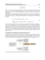
both algorithms have equivalent performances. This can be seen in Fig. 2, which presents
the symbol error rates at the output of ML space-time decoders fed with channel state
information (CSI) provided by KCE and SS-KCE, as well as at the output of an ML decoder
with perfect channel knowledge. Clearly, SS-KCE has the same performance of the KCE for
the two values of f
D
T
s
considered while demanding just a fraction of the complexity.
296
Adaptive Filtering Applications
Adaptive Channel Estimation in Space-Time Coded MIMO Systems 13


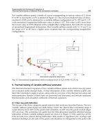
Fig. 1. Estimation mean squared error for KCE and SS-KCE.


Fig. 2. Symbol error rates of ML decoders fed with channel estimates provided by KCE and
SS-KCE.
We can explain the performance equivalence of KCE and SS-KCE by the fast convergence
of the matrix P
k|k−1
to its steady-state value. This means that the SS-KCE uses the optimal
297
Adaptive Channel Estimation in Space-Time Coded MIMO Systems
14 Will-be-set-by-IN-TECH
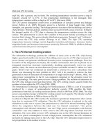
Fig. 3. Evolution of the entries of P
k|k−1
.
values of A

k
and B
k
after just a few blocks. Consequently, after these few blocks, the estimates
provided by the SS-KCE are the same as those generated by the optimal KCE. To exemplify the
fast convergence of P
k|k−1
, Fig. 3 shows the evolution of the values of the elements of P
k|k−1
for an 8-PSK, Alamouti coded system with N
R
= N
T
= 2, f
D
T
s
= 0.0015, p
r
= 0.4, p
t
= 0.8,
SNR
= 15 dB and with the initial condition P
0|0
= I
N
R
N
T

. It is clear from this figure that the
elements of the matrix P
k|k−1
reach their steady-state values before the transmission of 200
blocks. As the simulated system inserts 25 training blocks between 225 data blocks, we see
that P
k|k−1
converges even before the second training period. Due to the similar performances
of KCE and SS-KCE, we hereinafter present just SS-KCE results.
It is important to observe that the gap in the symbol error rate curves of Fig. 2, between the
decoders with perfect CSI and with estimated CSI, is due in great part to the use of the first
order AR approximation to the channel dynamics. To show this, in Fig. 4 we present the
symbol error rates at the output of decoders with perfect CSI and with SS-KCE estimates for
the same scenario used in Fig 2, except that in Fig. 4 the channel is also generated by a first
order AR process. As we can see, for f
D
T
s
= 0.0015, the receiver composed by SS-KCE and
the space-time decoder has the same performance as the ML decoder with perfect CSI. For
f
D
T
s
= 0.0075 and an SER of 10
−3
, the receiver using SS-KCE is about 5 dB from the decoder
with perfect CSI. This value is half of that shown in Fig. 2.
To analyze the impact of spatial channel correlation in the performance of the channel
estimation algorithms, the next scenario simulates the transmission of QPSK symbols to

2 receive antennas using Alamouti’s code for a normalized Doppler rate of 0.0045. The
receiver correlation coefficient p
r
is set to zero while the transmitter correlation coefficient
p
t
assumes values of 0.2 and 0.8. Fig. 5 presents the channel estimation MSE for SS-KCE and
RLS algorithms for both p
t
considered. From this figure, we note that the performances of
the estimation algorithms are hardly affected by transmitter spatial correlation and that the
298
Adaptive Filtering Applications
Adaptive Channel Estimation in Space-Time Coded MIMO Systems 15


Fig. 4. Symbol error rates of ML space-time decoders for a first order AR channel.
curves for RLS are indistinguishable. It is also clear that the SS-KCE performs much better
than the classical RLS algorithm. The symbol error rates at the output of ML decoders using
the channel estimates provided by SS-KCE and RLS filters are shown in Fig. 6. Since the
simulated RLS adaptive filter is not able to track the channel variations, the decoder can not
correctly decode the space-time codewords, leading to a poor receiver performance. On the
other hand, the receiver fed with SS-KCE estimates is 3 dB from the decoder with perfect CSI
for both values of p
t
at an SER of 10
−4
.
In the previous simulations, the channel estimators tracked simultaneously the 4 possible
channels between 2 transmit and 2 receive antennas. If the number of antennas increases, the

number of channels to be tracked simultaneously also increases. To illustrate the capacity of
the KF-based algorithms to track a larger number of channels, we simulate a system sending
QPSK symbols from N
T
= 4transmittoN
R
= 4 receive antennas. We employ the 1
/
2 -rate
OSTBC of (Tarokh et al., 1999) and assume p
t
= 0.8 and p
r
= 0.4. The MSE for the RLS and
the SS-KCE is shown in Fig. 7. We observe that the estimates produced by the RLS algorithm
are affected by the rate of channel variation. Moreover, the RLS MSE flattens out for SNR’s
greater than 10 dB. On the other hand, for this scenario, the SS-KCE has the same performance
for both values of f
D
T
s
considered and the MSE presents a linear decrease with the SNR. The
similar performances of SS-KCE for f
D
T
s
= 0.0015 and f
D
T
s

= 0.0045 are also reflected in
the symbol error rates at the output of the ML decoders, as shown in Fig. 8. For an SER of
10
−3
, the decoders using the channels estimates provided by the SS-KCE are about 1 dB from
the curves of the ML decoders with perfect CSI. For an SER of 10
−3
and f
D
T
s
= 0.0015 the
decoder fed with RLS channels estimates is approximately 4 dB from the optimal decoder,
while for f
D
T
s
= 0.0045 the RLS-based decoder presents an SER no smaller than 10
−1
in the
simulated SNR range.
To cope with the modeling error introduced by the use of the first-order AR channel model, we
show the FM-KCE in Section 5. Hence, to illustrate the performance improvement of FM-KCE
299
Adaptive Channel Estimation in Space-Time Coded MIMO Systems
16 Will-be-set-by-IN-TECH


Fig. 5. Estimation mean square error for different transmitter correlation coefficient.



Fig. 6. Symbol error rate for different transmitter correlation coefficient.
in comparison to the SS-KCE, we simulate a MIMO system with 2 transmit antennas sending
Alamouti-coded QPSK symbols to 2 receive antennas. The normalized Doppler rate is set to
0.0015, the receiver correlation coefficient p
r
is set to zero while the transmitter correlation
coefficient assumes the value p
t
= 0.4. We vary the number of training codewords from 4
300
Adaptive Filtering Applications
Adaptive Channel Estimation in Space-Time Coded MIMO Systems 17


Fig. 7. Estimation mean square error for different values of f
D
T.


Fig. 8. Symbol error rate for different values of f
D
T.
to 32 while maintaining the total number of blocks (training + data) fixed to 160 codewords.
Also, we assume the weight of the FM-KCE α
= 1.1.
In Fig. 9 we present the estimation MSE for SS-KCE and for the steady-state version of
FM-KCE, computed from the solution of the Riccati equation (41), with 4, 8, 12, 16, 20, 24, 28
and 32 training codewords. The arrows in this figure indicate the number of training
301

Adaptive Channel Estimation in Space-Time Coded MIMO Systems
18 Will-be-set-by-IN-TECH
0 5 10 15 20 25 30
10
10
10
10
10
SNR (dB)
MSE


SS-FM-KCE
SS-KCE
Fig. 9. Estimation mean square error for SS-KCE and FM-KCE.
codewords in ascending order. From Fig. 9, it is evident the superiority of FM-KCE over
SS-KCE. Differently from SS-KCE, whose performance improves with the increase in the
number of training codewords, the FM-KCE presents similar performances for the whole
range of training codewords considered. For instance, for an MSE of 10
−2
the FM-KCE
performs 5 dB better than the SS-KCE with 4 training codewords and about 3.5 dB better than
the SS-KCE with 32 traininig codeowrds.
The superior performance of the FM-KCE can also be observed in Fig. 10, which shows the
SER at the output of ML decoders fed with CSI provided by SS-KCE and FM-KCE, as well as
with perfect channel knowledge, for different training sequence lengths. For an SER of 10
−3
,
the receiver with the FM-KCE is about 0.8 dB from the decoder with perfect CSI, while the
receiver using channel estimates provided by the SS-KCE presents performance losses of 3

and 5.5 dB from the decoder with perfect CSI for 32 and 4 training codewords, respectively.
For an SER of 10
−4
, the receiver with the FM-KCE performs 2 and 3.5 dB better than the
receiver with SS-KCE for 32 and 4 training codewords, respectively, and presents a loss of
0.5 dB from the ML space-time decoder with perfect CSI. Thus, from Figs. 9 and 10, we see that
the FM-KCE allows the use of a small number of training codewords without compromising
the performance of the receiver.
7. Summary
In this chapter, we presented channel estimation algorithms intended for systems employing
orthogonal space-time block codes. Before developing the channel estimators, we construct a
state-space model to describe the dynamic behavior of spatially correlated MIMO channels.
Using this channel model, we formulate the problem of channel estimation as one of state
302
Adaptive Filtering Applications
Adaptive Channel Estimation in Space-Time Coded MIMO Systems 19
0 5 10 15 20 25 30
10
10
10
10
10
10
10
SNR (dB)
SER


Perfect CSI
SS-FM-KCE

SS-KCE
4 training
codewords
4 to 32 training
codewords
32 training
codewords
Fig. 10. Symbol error rate for SS-KCE and FM-KCE.
estimation. Thus, by applying the well-known Kalman filter to that state-space model, and
using the orthogonality of OSTBCs, we arrive at a low-complexity optimal Kalman channel
estimator. We also show that the channel estimates provided by the KCE in fact correspond to
weighted sums of instantaneous maximum likelihood channel estimates.
For constant modulus signal constellations, a reduced complexity estimator is give by
the steady-state Kalman filter. This filter also generates channel estimates by averaging
instantaneous ML channel estimates. The existence and stability of the steady-state Kalman
channel estimator is intimately related to the existence of solutions to the discrete algebraic
Riccati equation derived from the KCE.
Simulation results indicate that the SS-KCE performs nearly as well as the optimal KCE,
while demanding just a fraction of the calculations. They also show that the fading memory
estimator outperforms the traditional Kalman filter by as much as 5 dB for a symbol error rate
of 10
−3
.
8. Acknowledgments
We acknowledge the financial support received from CAPES.
9. References
Alamouti, S. M. (1998). A Simple Transmit Diversity Technique for Wireless Communications,
IEEE Journal on Selected Areas in Communications 16(10): 1451–1458.
Anderson, B. D. O. & Moore, J. B. (1979). Optimal Filtering, Prentice-Hall.
303

Adaptive Channel Estimation in Space-Time Coded MIMO Systems
20 Will-be-set-by-IN-TECH
Balakumar, B., Shahbazpanahi, S. & Kirubarajan, T. (2007). Joint MIMO Channel Tracking
and Symbol Decoding Using Kalman Filtering, IEEE Transactions on Signal Processing
55(12): 5873–5879.
Duman, T. M. & Ghrayeb, A. (2007). Coding for MIMO Communication Systems, John Wiley and
Sons.
Enescu, M., Roman, T. & Koivunen, V. (2007). State-Space Approach to Spatially Correlated
MIMO OFDM Channel Estimation, Signal Processing 87(9): 2272–2279.
Gantmacher, F. R. (1959). The Theory of Matrices, Vol. 1, AMS Chelsea Publishing.
Golub, G. H. & Van Loan, C. F. (1996). Matrix Computations, 3 edn, John Hopkins University
Press.
Haykin, S. (2002). Adaptive Filter Theory, 4 edn, Prentice-Hall.
Horn, R. A. & Johnson, C. R. (1991). Topics in Matrix Analysis, Cambridge University Press.
Jakes, W. C. (1974). Microwave Mobile Communications, John Wiley and Sons.
Jamoos, A., Grivel, E., Bobillet, W. & Guidorzi, R. (2007). Errors-In-Variables-Based Approach
for the Identification of AR Time-Varying Fading Channels, IEEE Signal Processing
Letters 14(11): 793–796.
Kailath, T., Sayed, A. H. & Hassibi, B. (2000). Linear Estimation, Prentice Hall.
Kaiser, T., Bourdoux, A., Boche, H., Fonollosa, J. R., Andersen, J. B. & Utschick, W. (eds) (2005).
Smart Antennas – State of the Art, Hindawi Publishing Corporation.
Komninakis, C., Fragouli, C., Sayed, A. H. & Wesel, R. D. (2002). Multi-Input
Multi-Output Fading Channel Tracking and Equalization Using Kalman Estimation,
IEEE Transactions on Signal Processing 50(5): 1065–1076.
Larsson, E. & Stoica, P. (2003). Space-Time Block Coding for Wireless Communications,Cambridge
University Press.
Larsson, E., Stoica, P. & Li, J. (2003). Orthogonal Space-Time Block Codes: Maximum
Likelihood Detection for Unknown Channels and Unstructured Interferences, IEEE
Transactions on Signal Processing 51(2): 362–372.
Li, X. & Wong, T. F. (2007). Turbo Equalization with Nonlinear Kalman Filtering for

Time-Varying Frequency-Selective Fading Channels, IEEE Transactions on Wireless
Communications 6(2): 691–700.
Liu, Z., Ma, X. & Giannakis, G. B. (2002). Space-Time Coding and Kalman Filtering for
Time-Selective Fading Channels, IEEE Transactions on Communications 50(2): 183–186.
Loiola, M. B., Lopes, R. R. & Romano, J. M. T. (2009). Kalman Filter-Based Channel Tracking in
MIMO-OSTBC Systems, Proceedings of IEEE Gl obal Communications Conference, 2009 –
GLOBECOM 2009., IEEE, Honolulu, HI.
Piechocki, R. J., Nix, A. R., McGeehan, J. P. & Armour, S. M. D. (2003). Joint
Blind and Semi-Blind Detection and Channel Estimation for Space-Time Trellis
Coded Modulation Over Fast Faded Channels, IEE Proceedings on Communications
150(6): 419–426.
Simon, D. (2006). Optimal State Estimation - Kalman, H
∞
, and Nonlinear Approaches, John Wiley
and Sons.
Tarokh, V., Jafarkhani, H. & Calderbank, A. R. (1999). Space-Time Block Codes from
Orthogonal Designs, IEEE Transactions on Information Theory 45(5): 1456–1467.
Vucetic, B. & Yuan, J. (2003). Space-Time Coding, John Wiley and Sons.
304
Adaptive Filtering Applications
14
Adaptive Filtering for Indoor Localization
using ZIGBEE RSSI and LQI Measurement
Sharly Joana Halder
1
, Joon-Goo Park
2
and Wooju Kim
1


1
Yonsei University, Seoul
2
Kyungpook National University, Daegu
Republic of Korea
1. Introduction

The term “filter” is often used to describe a device in the form of a piece of physical
hardware or computer software that is applied to a set of noisy data in order to extract
information about a prescribed quantity of interest [25], [26]. Filter has been designed to take
noisy data as input to reduce the effects of noise as much as possible.
A Wireless Sensor Network (WSN) is a network that consists of numerous small devices that
are in fact tiny computers. These so-called nodes are composed of a power supply, a processor,
different kinds of memory and a radio transceiver for communication. WSNs are generally
used to observe or sense the environment in a non-intrusive way. In order to perform this task,
nodes are often extended with sensors, like infrared, ultrasonic or temperature sensors, hence
the names sensor nodes and sensor networks. The domain of WSNs is still very young. During
the last few years, new developments in the area of communication, computing and sensing
have enabled and stimulated the miniaturization and optimization of computer hardware.
These evolutions have led to the emergence of WSNs. Despite the increasing capabilities of
hardware in general, sensor nodes are still very restricted devices. They have a limited amount
of processing power, memory capacity and most importantly energy. This makes WSNs a
challenging research topic.
Despite current restrictions, several applications for WSNs have already been designed.
WSNs are currently found in very different domains [3]. The large literature can be
classified by relying on several criteria. One of these is the physical means used for
localization, e.g., through the RF attenuation in the Electro-Magnetic (EM) waves [4], [11],
[13] (Received Signal Strength Indicator - RSSI - based techniques) or the time required to
cover the distance between transmitter and receiver (Ultra Wide Band); if using ultrasonic
pulses, one could also use the time of arrival or time-difference of arrival of the waves [10].

This can even be extended to Audible-frequency sounds [9]. Another classification is based
on the ranging feature, where distinguish between Range-free and Range-based localization
techniques [11]. Moreover, it can be classified according to the Single-hop [11] and Multi-
hop [14] localization scheme. Finally, it can differentiate between centralized [14] and
distributed [9] localization systems.
A common consensus among localization researchers is that indoor localization requires
room-level accuracy. Indoor localization uses many different sensors such as infrared, RFID,
Ultrasound, Ultra-Wide Band, Bluetooth, and WLAN. Different sensors provide different

Adaptive Filtering Applications

306
range of accuracy from centimeters to room-level. It seems like the accuracy is smaller than a
room. But in practice, when we directly transform (x,y), it coordinates to room-level
information and causes mistakes. The reason being is, wireless signal is easy to suffer
disturbance that makes localization unusual. This causes jumping in a split second or over a
short span. Such situation may effect the location estimation from one room to another.
Ubiquitous indoor environments often contain substantial amounts of metal and other such
reflective materials that affect the propagation of radio frequency signals in non-trivial ways,
causing severe multipath effects, dead-spots, noise and interference. The main focus of this
scheme is to represents a cheap and enhanced ranging technique to measure the radio strength
by using two useful radio hardware link quality metrics named Link Quality Indicator (LQI)
and Received Signal Strength Indicator (RSSI). In this scheme the mobile device itself calculate
the position. Moreover, the device calculates its own position based on its own measurements.
The proposed protocol tries to improve the existing algorithms [4], [27] using RSSI and LQI
values. The indoor localization systems presented in this report are based on the RSSI as a
strength indicator and LQI as a quality indicator of received packets. It can also be used to
estimate a distance from a node to reference points. This system uses the LQI and RSSI in a
different way and therefore it could lead to better and more predictable results than the
other existing system. Several experiments were conducted to investigate the performance

of the proposed scheme. At first, this system performs with respect to the signal analysis
to understand the characteristic of the LQI and RSSI values on three types of
environments to decide how the environment effects on RSSI and LQI strength. The effect
of distance on received signal strength can be measured by RSSI and LQI provided by the
radio. Secondly, this scheme performs with respect to the signal analysis is to filter the
original signals in order to remove the noise. Besides, the noise could be estimated by
using adaptive filtering algorithms. Sudden peaks and gaps in the signal strength are
removed and the whole signal is smoothed, which eases the analysis process. We used
two different types of new filtering to smooth the real RSSI, ‘LQI’ filtering and ‘BOTH’
filtering, and compared the results. And we found that ‘BOTH’ filter smooth more the raw
RSSI value than existing ‘Fusion’ filtering [27].
In our research we used an adaptive filter as it performs well to track an object under such
changing conditions in the RF signal environment. In this chapter, the proposed protocol
will try to improve the existing algorithms using RSSI and LQI values. The localization
systems presented in this report are based on RSSI as a strength indicator and LQI as a
quality indicator of a received packets, it can also be used to estimate a distance from a node
to reference points.
The remainder of this Chapter consists of six sub chapters. Chapter 2 describes some
properties of ZigBee, RSSI and LQI. Chapter 3 reveals the previous works based on indoor
location and WSN. Chapter 4 provides the proposed model of “Adaptive Filtering for
Indoor Localization using ZIGBEE RSSI and LQI Measurement” and its probability of
returning the correct location. Chapter 5 describes the analytical results obtained from the
model of location system. And Chapter 6 concludes the chapter with conclusions.
2. ZigBee, RSSI and LQI
2.1 ZigBee
There are several standards that address mid to high data rates for voice, PC LANs, video,
etc. and until recently there has not been a wireless network standard that meets the unique

Adaptive Filtering for Indoor Localization using ZIGBEE RSSI and LQI Measurement


307
needs of devices such as sensors and control devices. Sensors and control devices which are
mostly used in industries and homes distinguish them with low data rates and in needs of
very low energy consumption. A standards-based wireless technology needed having the
performance characteristics that closely meet the requirements for reliability, security, low
power and low cost.
Table 1 presented the IEEE 802.15 Task Group 4 is chartered to investigate a low data rate
solution with multi-month to multi-year battery life and very low complexity. It is intended
to operate in an unlicensed, international frequency band.
Since low total system cost is a main issue in industrial and home wireless applications, a
highly integrated single-chip approach is the preferred solution of semiconductor
manufacturers developing IEEE 802.15.4 compliant transceivers. The IEEE standard at the
PHY is the significant factor in determining the RF architecture and topology of ZigBee
enabled transceivers. For these optimized short-range wireless solutions, the other key
element above the Physical and MAC Layer is the Network/Security Layers for sensor and
control integration. The ZigBee group was organized to define and set the typical solutions
for these layers for star, mesh, and cluster tree topologies.

Feature(s) IEEE 802.11b Bluetooth ZigBee
Power Profile Hours Days Years
Complexity Very Complex Complex Simple
Nodes/Master 32 7 64000
Latency Enumeration upto 3 sec Enumeration upto 10 sec Enumeration 30 ms
Range 100 m 10m 70m~300m
Extendability Roaming possible No Yes
Data Rate 11Mbps 1Mbps 250Kbps
Security
Authentication Service
Set ID (SSID)
64 bit, 128 bit

128 bit AES and
Application Layer
user defined
Table 1. Comparison of key features of complementary wireless technologies [4]
ZigBee Applications:
ZigBee is the wireless technology that:
 Enables broad-based deployment of wireless networks with low cost, low power
solutions [5].
 Provides the ability to run for years on inexpensive primary batteries for a typical
monitoring application [5].
 Addresses the unique needs of remote monitoring & control, and sensory network
applications [5].
Figure 1 shows the ZigBee application areas. However, ZigBee technology is well suited to a
wide range of building automation, industrial, medical and residential control & monitoring
applications. Essentially, applications that require interoperability and/or the RF
performance characteristics of the IEEE 802.15.4 standard would benefit from a ZigBee
solution.

Adaptive Filtering Applications

308

Fig. 1. ZigBee applications [5].
2.2 Received signal strength indicator (RSSI)
Majority of the existing methods leverage the existence of IEEE 802.11 base stations with
powerful radio transmit powers of approximately 100mW per base station. Such radios are
in a different class from the low power IEEE 802.15.4 compliant radios that typically
transmit at low power levels ranging from 52mW to 29mW. The wide availability of larger
number of IEEE 802.15.4 radios has revived the interest for signal strength based localization
in sensor network. Despite of rapidly increasing popularity of IEEE 802.15.4 radios and

signal strength localization, there is a lack of detailed characterization of the fundamental
factors contributing to large signal strength variation. The analysis of RSSI values is needed
to understand the underlying features of location dependent RSSI patterns and location
fingerprints. An understanding of the properties of the RSSI values for location can assist in
improving the design of positioning algorithms and in deployment of indoor positioning
systems. The characteristics of RSS, received signal strength will decrease with increased
distance as the equation below shows:
RSSI = − (10nlog
10
d + A) (1)
Where,
n = signal propagation constant, also named propagation exponent.
d = distance from sender.
A = received signal strength at a distance of one meter.
Lots of localization algorithms require a distance to estimate the position of unknown
devices. One possibility to acquire a distance is measuring the received signal strength of the
incoming radio signal.
The idea behind RSS is that the configured transmission power at the transmitting device
(PTX) directly affects the receiving power at the receiving device (PRX). According to Friis’
free space transmission equation, the detected signal strength decreases quadratically with
the distance to the sender (Figure 2.a).
PRX = PTX * GTX * GRX (λ/4πd)
2
(2)

Adaptive Filtering for Indoor Localization using ZIGBEE RSSI and LQI Measurement

309

(a) (b)

Fig. 2. (a) Received power PRX versus distance to the transmitter. (b) RSSI as quality
identifier of the received signal power PRX.
Where,
PTX = Transmission power of sender
PRX = Remaining power of wave at receiver
GTX = Gain of transmitter
GRX = Gain of receiver
λ = Wave length
d = Distance between sender and receiver
In embedded devices, the received signal strength is converted to a received signal strength
indicator (RSSI) which is defined as ratio of the received power to the reference power
(PRef). Typically, the reference power represents an absolute value of Pref =1mW.
RSSI = 10 * log PRX/PRF [RSSI] = dBm (3)
An increasing received power results a rising RSSI. Figure 2.b illustrates the relation
between RSSI and the received signal power. Plotting RSSI versus distance d results in a
graph, which is in principle axis symmetric to the abscissa. Thus, distance d is indirect
proportional to RSSI. In practical scenarios, the ideal distribution of PRX is not applicable,
because the propagation of the radio signal is interfered with a lot of influencing effects.
2.3 Link quality indicator (LQI)
For communications IEEE 802.15.4 radios provide applications with information about the
incoming signal [17]. The effect of distance on received signal strength (RSS) can be
measured by the packet success rate, RSSI and LQI provided by the radio. LQI is a metric
introduced in IEEE 802.15.4 that measures the error in the incoming modulation of
successfully received packets (packets that pass the CRC criterion). The LQI metric
characterizes the strength and quality of a received packet. It is introduced in the 802.15.4
standard [1] and is provided by CC2430 [17]. LQI measures each successfully received
packet and the resulting integer ranges from 0x00 to 0xff (0-255), indicating the lowest and
highest quality signals detectable by the receiver (between -100dBm and 0dBm). The
correlation value of LQI range from 50 to 110 where 50 indicates the minimum value and


Adaptive Filtering Applications

310
110 represents the maximum. The 50 is typically the lowest quality frames detectable by
CC2430. Software must convert the correlation value to the range 0-255, e.g. by calculating:
LQI = (CORR – a) · b (4)
Where,
CORR= correlation value, a and b are found empirically
The CORR (correlation value) is the raw LQI value which can be obtained from the last byte
of the message. The raw value can get from CC2430 (CORR) is between 40 and 110.
Limited to the range 0-255, where a and b are found empirically based on PER
measurements as a function of the correlation value. A combination of RSSI and correlation
values may also be used to generate the LQI value. LQI values are uniformly distributed
between these two limits. Different form RSSI, LQI measures the qualities of links while
RSSI measures the strengths of links. LQI is a measure of the error in the signal, not the
strength of the signal. A “weak” signal may still be a very crisp signal with no errors and
thus a potentially good routing neighbor. If there is no interference from other 2.4 GHz
devices, then LQI will generally be good over distance. Note that, scaling the link quality to
a LQI, compliant with IEEE 802.15.4, must be done by software. This can be done on the
basis of the RSSI value, the correlation value or a combination of those two. Signal strength
and link quality values are not necessarily linked. But if the LQI is low, it is more likely that
the RSSI will be low as well. Nevertheless, they also depend on the emitting power. A
research group had the following results:


Low RF High RF
LQI
105 108
RSSI
- 75dBm - 25dBm


Even though they do not describe how far from each other the sender and the receiver are
located, it illustrates perfectly that both low and high power emissions guarantee a good
link quality. The low RF emissions could be more sensitive to external disturbances. LQI
exhibits a very good correlation with packet loss, and is therefore a good link quality
indicator. However, one of the contributions of the present work is to show that RSSI is a
reasonable metric if it is processed correctly, and if interference can be distinguished from
noise. Given that LQI is a superior metric, it should not be forgotten that it is only made
available by 802.15.4-compliant devices. It therefore makes sense to make the most out of
RSSI.
3. Related works
This chapter introduces the area of ubiquitous computing and the underlying sensing
technologies such as ultrasonic, infrared, Global Positioning Systems, and radio frequency
identification. At first, an brief overview of each of the systems is given and then the
similarities and differences to the approach are discussed.
3.1 Terminology and principles
There are numbers of existing location systems which utilize a variety of sensing
technologies and system architectures. These systems have varying characteristics, such as
accuracy, scalability, range, power consumption and cost. This section describes some of the

Adaptive Filtering for Indoor Localization using ZIGBEE RSSI and LQI Measurement

311
sensor terminology and principles used with reference to location systems. There are a
number of different sensor technologies have been used in location systems.
3.1.1 Light
Light is a widely-used medium in location systems, varying from the use of simple infrared
LEDs and sensors to tag-less vision based tracking. Infrared has been popularly used for
containment-based location systems [20]. Infrared location systems can suffer in strong
sunlight and under fluorescent tube lighting as both of these are sources of infrared light.

Video cameras can be used both to recognize objects within the environment, allowing the
device to calculate its position, or as an infrastructure to track mobile objects which may or
may not be augmented. The processing power required to track objects, especially if they are
untagged, using image-based methods can be large compared to other methods.
3.1.2 Radio-based localization
Localization in sensor networks can be achieved using knowledge about the radio signal
behavior and the reception characteristics between two different sensor nodes. The quality
of a radio signal, i.e. its strength at reception time, is expressed by RSSI: the higher the RSSI-
value, the better the signal reception. The main advantage of using radio-based localization
techniques is that no additional hardware for the sensor nodes is required. The main
disadvantage of the technique is that the measured signal strengths are generally unstable
and variable over time, which leads to localization errors. In this section, two common
localization techniques using radio signal strength information are presented. Afterwards,
the proximity idea is discussed, a technique that takes into account the range of radio
communication rather than its quality. Finally, a technique for analyzing the RSSI behavior
over time is presented. The technique cannot be used for localization itself, but it can
provide useful mobility information about the node to be located. Following are three types
of radio-based localization systems:
3.1.2.1 Converting signal strength to distance
In theory, there exists an exponential relation between the strength of a signal sent out by a
radio and the distance the signal has traveled. In reality, this correlation has proven to be
less perfect, but it still exists. Reference nodes broadcast a message to inform their position
at regular intervals. Unknown nodes receive the broadcast message from reference nodes
and measure the strength of the received signal [4], [27], [28]. Localization errors for this
method range from two to three meters at average, with indoor errors being larger than
outdoor ones. The main reason for the large number of errors is that the effective radio-
signal propagation properties differ from the perfect theoretical relation that is assumed in
the algorithm. Reflections, fading and multipath effects largely influence the effective signal
propagation. The distance estimates, which are based on the theoretical relation, are thus
inaccurate and lead to high errors in the calculated locations.

3.1.2.2 Fingerprinting signal strength
The second method that uses RSSI for localization is called Fingerprinting. This technique is
based on the specific behavior of radio signals in a given environment, including reflections,
fading and so on, rather than on the theoretical strength-distance relation. The
fingerprinting technique [11], [12], [15] is an anchor-based technique that consists of two
separate phases. During the first phase, called the Offline Phase, a fingerprint database of

Adaptive Filtering Applications

312
the environment is constructed. During the next phase, called the Online Phase, real-time
localization is performed. The greatest disadvantage of the fingerprints method is that an
offline phase is required for the system to work. The offline phase is very time consuming.
Moreover, the fingerprinting database that is created during the offline phase is location
dependent. If one wants to use the same system in another environment or if radical
changes to the current environment are made, the offline phase has to be repeated.
3.1.2.3 Proximity-based localization
Proximity-based localization systems are an anchor-based solution to the localization
problem. These systems derive their location data from connectivity information of the
network [4], [7], [8], [11], [12], [23]. Knowledge about whether two devices, i.e. an unknown
node and an anchor, in the network are within communication range is transformed into an
assumption about their mutual distance and location.
3.1.3 Ultrasound
The propagation speed of ultrasound waves in air is slow compared to that of RF. Sound
waves are generally reflected by objects in the environment, which also makes position by
containment possible. Utilizing the differential time-of-flight between RF and ultrasound
pulses allows position to be estimated to within a few centimeters of the ground truth. The
attenuation of sound in air limits range to several meters. Sound waves generally take about
20ms to die out; this therefore limits the update rate ultrasound location systems can obtain.
The prevalent frequency used in ultrasound ranging is ultrasound. A lot of ultrasound

location systems have been developed using narrow band 40 kHz transducers [10], [21].
Following are three types of ultrasound based localization systems:
3.1.3.1 The bat ultrasonic location system
Bat system provides fine-grain 3D location and orientation information which its
predecessor, the Active Badge System, did not. Position is calculated using trilateration. The
Bat emitter will transmit a short ultrasound pulse and receivers placed at 1.5m apart at
known locations on the ceiling will pick up the signals [16].
3.1.3.2 Cricket
Cricket [10] is an indoor location system developed at MIT and utilizes RF and ultrasound
using static transmitters and mobile receivers. The first iteration of the system is
containment-based allowing for areas of arbitrary size to be created via careful placement of
transmitters in the environment. A later iteration, called Cricket Compass [22], set out to
allow orientation as well as position to be determined.
3.1.3.3 Dolphin
The Dolphin system [21], developed at the University of Tokyo, utilizes both RF and
ultrasound to create a peer-to-peer system, providing co-ordinate based positioning. The
aim is to develop a system which is easy to configure and provides a high degree of
accuracy in three dimensions.
3.1.4 Adhoc positioning system (APS) using AoA
Niculescu and Nath [6] aim to create an algorithm and simulate a system where nodes have
highly directional detection capabilities and there exist a small number of seeded nodes.
Different algorithms were simulated in this chapter to gain some insight into how systems

Adaptive Filtering for Indoor Localization using ZIGBEE RSSI and LQI Measurement

313
with different properties would behave. The data suggests that higher node densities
increase the probability of node connectivity sufficiently to calculate location and
orientation. Smaller angles lower the error. However this reduces the percentage of nodes
for which locations are estimated.


3.1.5 Global positioning system (GPS)
The GPS system consists of twenty seven satellites that orbit the Earth [14], [24]. GPS use the
distance and angle measurements to the reference points are used to compute the position of
the object by triangulation. GPS uses the time of flight of RF signals to estimate the distance
between GPS satellites and receiver [24]. In indoor environments, GPS satellites signals get
attenuated and reflected by various metallic objects [24]. Indoor GPS performance has
fundamental limitations that result in much larger position estimation errors compared to
outdoors.
RSSI can provide us with the cheapest localization system possible, while the form factor of
the sensor nodes is not increased. The technique is applicable to indoor environment and the
errors achieved with a RSSI-based system seem to be promising compared to the more
expensive systems. In this chapter, we decided to design and implement a RSSI-based
system to solve the localization problem listed above. The main reason is that it can be
developed with small modifications to the existing systems.


Fig. 3. Taxonomy of positioning system.
3.1.6 Comparison
The following table provides a comparison of the surveyed sensing systems from the point
of accuracy and precision, scale, cost and limitations:
From Table 2, we concluded that RSSI can provide us with the cheapest localization system
possible, while the form factor of the sensor nodes is not increased. The technique is applicable
to indoor environment and the errors achieved with a RSSI-based system seem to be
promising compared to the more expensive systems. In this chapter, we decided to design and
implement a RSSI-based system to solve the localization problem listed here. The main reason
is that it can be developed with small modifications to the existing systems. However, the
aspects of accuracy and coverage area are still to be investigated in Chapter 4 and 5.

Adaptive Filtering Applications


314
GPS Infrared Ultrasound RSSI
Applicable indoor
Not
recommended
Yes Yes Yes
Need for extra
hardware
Yes Yes Yes No
Cost of extra
hardware
High Low High N.A
Size of extra
hardware
Average Average Large N.A
Average expected
error
± 10 meters ± 5 meters ± 10 meters 1~3 meters
Table 2. Comparison of different location sensing technologies [13]
4. Proposed scheme
This chapter will focus on how this effective protocol has been implemented, and
implementation issues are considered. In our experiments, to measure the radio strength,
two useful radio hardware link quality metrics were used: (i) LQI and (ii) RSSI. Specifically,
RSSI is the estimate of the signal power and is calculated over 8 symbol periods, while LQI
can be viewed as chip error rate and is calculated over 8 symbols following the start frame
delimiter (SFD). The specific point in a system where position estimates are calculated is an
important design parameter. In this scheme the mobile device itself calculate the position.
The device calculates its own position based on its own measurements.
4.1 Selected location system architecture

This scheme decides to use a private and scalable system. It features an active base station
that transmits both RSSI and LQI signals. The mobile devices receive the signals, but they do
not transmit anything themselves. The base station transmits the RSSI and LQI signals at the
same moment in time. A mobile device measures signal, and is able to calculate the distance
to the transmitter. By this scheme the location privacy of the user, who carries the mobile
device, can be easily guaranteed because the mobile device does not send out any signals
that might disclose its presence or its location. A further advantage of this architecture is
scalability to many mobile devices. Because the mobile devices do not transmit any signals,
there can be an unlimited number of mobile devices in principle. Due to its privacy and
scalability features, this architecture might be particularly suitable for large-scale
professional location systems or systems in public spaces. Each mobile device calculates its
own position, based on the received signals. This scheme has divided into two subsystems.
As we know, for environmental changes the log model also change, so the proposed system
uses a scaling factor for adjusting the log model with the measured data. This system
includes a scaling factor s with the basic RSSI log model equation.
RSSI = ─ 10 nlog
10
(sd + 1) + A (5)
Where,
s = scaling factor
For our experiment, we use a filtering process for smoothing the RSSI values. We proposed
a LQI filtering and BOTH filtering of RSSI and LQI values, for smoothing the measured

Adaptive Filtering for Indoor Localization using ZIGBEE RSSI and LQI Measurement

315
RSSI. From our experiment, we determine the filtering factor a for filtering and we used the
following equation for smoothing the measured RSSI.
smooth_RSSI
t(BOTH)

=a*RSSI
t
+(1-a)*RSSI
t-1
(6)
5. Experimental result
Adaptive filter contains a set of adjustable parameters. In design problem the requirement is
to find the optimum set of filter parameters from knowledge of relevant signal
characteristics according to some criterion.
This mathematical system combines the general principles of a proximity-based
localization system with the analysis of the radio signal strength behavior over distance.
This system uses the link quality indicator and radio signal strength indicator in a
different way and therefore it could lead to better and more predictable results than the
other existing system. Several experiments had conducted to investigate the performance
of the proposed scheme.
The first step of this system performs with respect to the signal analysis to understand the
characteristic of LQI and RSSI values on three types of environments. The effect of distance
on received signal strength can be measured by RSSI and LQI provided by the radio.
Equation 1 describes the basic model formula for RSSI where RSS decrease with increased
distance. As for environmental change the log model also changed, this scheme decided to
use a scaling factor s in the basic log model equation to adjust the log model with measured
RSSI values. So, to find the accurate log model for specific environment we use a scaling
factor s in equation 5. The experiment is conducted on three types of following environment
to decide how the environment effects on RSSI and LQI strength. The first experiment is
conducted in close space indoor environment.


Fig. 4. Close space indoor environment (path 1).
The second experiment is deployed in half open space indoor environment, where few
meters of the corridor was open.



Fig. 5. Half open space indoor environment (path 2).