Adaptive Filtering Applications
262
of ANFIS was introduced by J.S.R. Jang in his seminal paper in (Jang, 1993). It may be noted
that the equalization of wireless mobile channels is a non-linear problem, so that a non-
linear solution, such as ANFIS, is more appropriate. One has to design the fuzzy if-then else
rules based on the channel characteristics; namely variances of signal, noise, co-channel
(CCI) and adjacent channel interferences (ACI) as well as the transmitted signal (input)-
received signal (output) mapping. The equalizer is a non-linear system that effectively
undoes the aberrations done to the transmitted signal by the channel due to the noise and
co-channel and adjacent channel interferences. Now, the modeling a non-linear system is
fairly complex so that conventional methods of system identification techniques cannot be
applied to find the inverse system. One possible experimental method to develop a model
for indoor wireless channel (viz., the channel impulse response, CIR) is to carry out
expensive channel sounding (for example, one could use the RUSK Channel sounder from
RF Sub Systems, GmBH, which would cost over a hundred thousand dollars). In this article,
we attempt to supplant the expensive channel sounding technique for mobile wireless
channel (that too, not restricted to the indoor case) by suitable simulation techniques.
7.1 Introduction to ANFIS
Functionally, there are almost no constraints on the node functions of an adaptive network
except piecewise differentiability. Structurally, the only limitation of network configuration
is that it should be of feedforward type. Due to these minimal restrictions, the adaptive
network’s applications are immediate and immense in various areas. For simplicity, we
assume the fuzzy inference system under consideration has two inputs x and y and one
output z (Jang, 1993). Suppose that the rule base contains two fuzzy if–then rules of Takagi
and Sugeno’s type:
Rule1 : If x is A1 and y is B1, then f1 = p1x + q1y + r1. (2)
Rule2 : If x is A2 and y is B2, then f2 = p2x + q2y + r2. (3)

Fig. 4. The Takagi-Sugeno-Kang (TSK) Model of Fuzzy Reasoning. (a) Type-3 Fuzzy
Reasoning. (b) Equivalent ANFIS (Type—3 ANFIS).

An Introduction to ANFIS Based Channel Equalizers for Mobile Cellular Channels
263
The type–3 fuzzy reasoning is illustrated in Figure 4(a) and the corresponding equivalent
ANFIS architecture (type–3 ANFIS) is shown in Figure 4(b).
7.2 Mobile cellular channel equalization based on ANFIS
One can observe that wireless channel can be modeled as non-linear time-variant (NLTV)
when the duration of observation window is fairly long or as non-linear time invariant
(NLTI) when the duration of observation window is short. This fact is established by
simulation, as it is a hard problem to obtain a rigorous mathematical proof. Conventional
channel models available in recent literature were studied to arrive at a suitable paradigm
for the wireless channel, consisting of the different variables and parameters. This also
enabled us to understand the inadequacies of existing mathematical models for wireless
channels. The fuzzy if-then rules are generated by the inverse system based on ANFIS (to
the channel), which effectively acts as an adaptive equalizer at the receiver side. The
ANFIS automatically generate the rule base from a set of input-output data vectors. This
is achieved by minimizing the error between actual input signal (at the transmitter of the
wireless system) and the estimate of the input (at the receiver). In the simulation, we
assume that the external input to the ANFIS equalizer is the output of the channel, which
is the sum of the desired channel output plus the weighted sum of the co-channel outputs
and the Gaussian noise, which is assumed to be AWGN, with zero mean and standard
deviation upto 0.8. In the ensuing sections, we use the following definitions for Signal-to-
Noise Ratio (SNR), Signal-to-Interference Ratio (SIR) and Signal-to-Interference Noise
Ratio (SINR) (Liang & Mendel 2000):
SNR = 10 log
10
{
s

2
/
n
2
} (4)
SIR = 10 log
10
{
s
2
/
i
2
} (5)
SINR = 10 log
10
{
s
2
/(
i
2
+ 
n
2
)} (6)
where

s
2

,


n
2
, and


i
2
are the variances of the signal, AWG noise, and the co-channel and
adjacent channel interferences (put together) signal respectively.

T
y
pe
N
odes Linear/Nonlinear Parameters
F
uzz
y
Rules
ANFIS-17 32 14/14 7
ANFIS-115 64 30/30 15
ANFIS-125 104 50/50 25
ANFIS-25 75 75/20 25
ANFIS-27 131 147/28 49
ANFIS-35 286 500/30 125
ANFIS-37 734 1372/42 343
Table 1. Simulation Parameters for Various ANFIS Based Channel Equalizers

The output of the equalizer is given to a limiter to clip the output levels to limiting values of
+1 or −1. The different parameters of the various simulation setups are as tabulated in Table
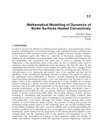
1. The structure of ANFIS–27 is given in Figure 5. The library function, anfis, available in the
Fuzzy Logic Toolbox of MATLAB® R2010b is used extensively in all simulations.

Adaptive Filtering Applications
264

Fig. 5. The Structure of ANFIS—27 Generated Using MATLAB Fuzzy Logic Toolbox.
Note that ANFIS–27 based equalizer has two inputs from multipath components, seven (7)
fuzzy rules for each input and one output that feed the receiver subsystem.


Fig. 6. The Equivalent ANFIS Architecture for Channel Equalizer.

An Introduction to ANFIS Based Channel Equalizers for Mobile Cellular Channels
265
The Figure 6 shows the architecture of the proposed ANFIS based channel equalizer, for 7
fuzzy rules. The wireless channel modeling based on artificial neural networks is capable
of depicting the input-output mapping existing in the equalizer system and it does
provide us with an exact picture of the variables and parameters defining the system.
Moreover, neural network based models do have the learning capability. The fuzzy
models, on the other hand, do not possess the learning capability. Therefore, fusing
together these two, we can have a model which is capable of both depicting the dynamics
of the system in terms of the variables and parameters and is having the self-learning
capability. The adaptability of the equalizer under purview is achieved by the learning
aspect of neural network. The fuzzy reasoning (especially the TSK model used in ANFIS)
maps the input to the output. We follow a first-order ANFIS with the antecedent
parameters being the standard deviations of the received signal, CCI and ACI
interferences (put together), and the AWGN (σ

s
, σ
i
, and σ
n
, respectively), collectively
represented as A
i
. The only consequent parameter is the scaling factor of the signal (ρ
i
) at
the output. The membership functions of A
i
, i = 1, 2,…, 7 are chosen to be Gaussian. Some
of the rules in the fuzzy rule base can be stated as:
If σ
s
is very low, and σ
i
is very low, and σ
n
is very low then y = ρ
1
s. (7)
If σ
s
is low, and σ
i
is very low, and σ
n

is very low then y = ρ
2
s. (8)
If σ
s
is medium, and σ
i
is very low, and σ
n
is very low then y = ρ
3
s. (9)
If σˆs is medium, and σ
i
is low, and σ
n
is low then y = ρ
4
s. (10)


Fig. 7. The Error Plot of ANFIS-125 Training.

Adaptive Filtering Applications
266
The three input variables can assume any one of the 5 possible membership functions from
the set, {very low, low, medium, high, very high}, leaving us with 125 possible combinations of
rules. However, using fuzzy rule reduction techniques the total number of rules can be limited
to 7 or 25. The steps in the algorithm for simulation of the ANFIS–27 based equalizer are as
given below:

1. The standard deviations of CCI and AWGN are logarithmically varied from 0.02 to 0.8.
This information is derived from literature.
2. The random binary input data (which represents the input to the channel from the
transmitter) is generated and the corrupted data available at the outputs of the two
multipaths due to CCI and AWGN is obtained.
3. Set the number of membership functions as 7, membership function type as “Gaussian”
and the number of epochs to 80.
4. Simulate the ANFIS (which implements the equalizer) and plot the results.
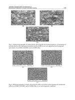
The error plot of the ANFIS–125 training is illustrated in Figure 7.
We have set the number of epochs as 80 in this case. As the ANFIS implementation in
MATLAB do not lend itself to observe the updation of Antecedent and consequent parameters, while
training is under progress, we can consider the training error as a reliable pointer to the step wise
updation of the above parameters. The ANFIS-125 consists of one input, one output, and 25
fuzzy rules for each membership functions.
7.3 The results of simulations of ANFIS based equalizers
The simulated output of the channel, which is the input to the ANFIS based channel
equalizer, along with the training data is shown in Figure 8. The output of the channel
(received signal), which is a non-linear combination of the signal, the co-channel signals,
and the AWG noise, is a random waveform taking values around +1 and −1, as seen from
the simulated waveform. The MATLAB code to generate the plot is given below.


Fig. 8. The Training Data Pair for ANFIS-125 Equalizer Simulation.

An Introduction to ANFIS Based Channel Equalizers for Mobile Cellular Channels
267
The equalized, output after thresholding, will be very much identical to the training data as
shown in Figure 9.



Fig. 9. Simulation Results for ANFIS-125 and ANFIS-127 based Equalizers.
%% MATLAB Code for ANFIS Equalizer Simulation with 1 input and 5
%% membership functions /1 input and 25 membership functions.
% Last modified on 13-03-2011.
clear all; clf;
tic;
ns=1024;
nb=4;
t=[1:ns*nb];
[x,b] = random_binary(ns,nb);
[x1,b1] = random_binary(ns,nb);
[x2,b2] = random_binary(ns,nb);
[x3,b3] = random_binary(ns,nb);
[x4,b4] = random_binary(ns,nb);
[x5,b5] = random_binary(ns,nb);
[x6,b6] = random_binary(ns,nb);
e=0.2*randn(ns*nb,1);
y1 = x'+0.2*(x1'+x2'+x3'+x4'+x5'+x6')+e;
trnData = [y1 x'];
numMFs = 25;
mfType = 'gaussmf';
epoch_n = 20;

Adaptive Filtering Applications
268
subplot(211),plot(t(512:1024),y1(512:1024),'k');
axis([512 1024 -5 5]); grid on;
xlabel('Time t');ylabel('Amplitude');
legend('Channel output, x[k] Input to the Equalizer');
title('Training Data Pair for ANFIS-125 and ANFIS-127');

subplot(212),plot(t(512:1024),x(512:1024),'k');
axis([512 1024 -1.5 1.5]); grid on;
xlabel('Time t');ylabel('Amplitude');
legend('Training Data');
%%%%
%% ANFIS Equalizer Simulation with 1 input and 5 membership
%% functions /1 input and 25 membership functions.
% Last modified on 13-03-2011.
clear all;clf;
tic;
ns=1024;
nb=4;
t=[1:ns*nb];
[x,b] = random_binary(ns,nb);
[x1,b1] = random_binary(ns,nb);
[x2,b2] = random_binary(ns,nb);
[x3,b3] = random_binary(ns,nb);
[x4,b4] = random_binary(ns,nb);
[x5,b5] = random_binary(ns,nb);
[x6,b6] = random_binary(ns,nb);
e=0.2*randn(ns*nb,1);
y1 = x'+0.2*(x1'+x2'+x3'+x4'+x5'+x6')+e;

trnData = [y1 x'];
numMFs = 25;
mfType = 'gaussmf';
epoch_n = 20;
in_fismat = genfis1(trnData,numMFs,mfType);
out_fismat = anfis(trnData,in_fismat,20);
est_x125=evalfis(y1,out_fismat);


est_x125(est_x125<-0.6)=-1.0;
est_x125(est_x125>0.6)=1.0;

trnData = [y1 x'];
numMFs = 27;
mfType = 'gaussmf';
epoch_n = 20;
in_fismat = genfis1(trnData,numMFs,mfType);
out_fismat = anfis(trnData,in_fismat,20);
est_x127=evalfis(y1,out_fismat);

An Introduction to ANFIS Based Channel Equalizers for Mobile Cellular Channels
269

est_x127(est_x127<-0.6)=-1.0;
est_x127(est_x127>0.6)=1.0;

subplot(311),plot(t(512:1024),x(512:1024),'k');
axis([512 1024 -1.5 1.5]); grid on;
xlabel('Time t');ylabel('Amplitude');
title('Training Data for ANFIS-125 and ANFIS-127');

subplot(312),plot(t(512:1024),est_x125(512:1024),'k');
axis([512 1024 -1.5 1.5]); grid on;
xlabel('Time t');ylabel('Amplitude');
legend('Detector Output for ANFIS-125');
title('Simulation Results for 1 input and 25 membership functions');

subplot(313),plot(t(512:1024),est_x127(512:1024),'k');

axis([512 1024 -1.5 1.5]); grid on;
xlabel('Time t');ylabel('Amplitude');
legend('Detector Output for ANFIS-127');
title('Simulation Results for 1 input and 27 membership functions');
toc;
%%%%%

In one of the simulations, the standard deviation of CCI and AWGN are logarithmically
varied between 0.02 and 0.8and simulation is run on a total of 2048/4096 training data pairs.
The results are shown in Figure 10. The MATLAB code to generate the same is appended
below.


Fig. 10. Performance of ANFIS based Equalizer—Logarithm of BER at output versus SNR in
dBs.

Adaptive Filtering Applications
270
% %% Modified ANFIS Equalizer Simulation
% % with more precision. Plots Logarithm of BER versus SINR
% std of CCI varied from 0.02 to 0.8.
% std of AWGN varied from 0.02 to 0.8.
%%% last modified on 13-03-2011.
%anfis15.m
clc;clf;clear;close;
tic;
nb=1024;
ns=4;
it=20;
% t=linspace(0.02,0.8,it);

t=logspace(log10(0.02),log10(0.8),it);
[x,b] = random_binary(nb,ns);
[x1,b1] = random_binary(nb,ns);
[x2,b2] = random_binary(nb,ns);
[x3,b3] = random_binary(nb,ns);
[x4,b4] = random_binary(nb,ns);
[x5,b5] = random_binary(nb,ns);
[x6,b6] = random_binary(nb,ns);
i=1;
cci=x1+x2+x3+x4+x5+x6;
noise=randn(ns*nb,1);
for j=1:it
e=noise*t(j);
z=cci*t(j);
sinr(i)=10*log10(var(x)/(var(z)+var(e)));
y = x'+z'+e;
trnData = [y x'];
numMFs = 5;
mfType = 'gaussmf';
epoch_n = 20;
in_fismat = genfis1(trnData,numMFs,mfType);
out_fismat = anfis(trnData,in_fismat,20);
est_x=evalfis(y,out_fismat);
est_x(est_x<-0.6)=-1.0;
est_x(est_x>0.6)=1.0;
ec=(x~=est_x');
ber(i)=sum(ec)/(nb*ns);
i=i+1;
end;
plot(sinr, log10(ber),'-+');hold on;grid on;

xlabel('SINR in dB');
ylabel('Logarithm of BER');
%end of ANFIS15;
i=1;
for j=1:it

An Introduction to ANFIS Based Channel Equalizers for Mobile Cellular Channels
271
e=noise*t(j);
z=cci*t(j);
sinr(i)=10*log10(var(x)/(var(z)+var(e)));
y = x'+z'+e;
trnData = [y x'];
numMFs = 7;
mfType = 'gaussmf';
epoch_n = 20;
in_fismat = genfis1(trnData,numMFs,mfType);
out_fismat = anfis(trnData,in_fismat,20);
est_x=evalfis(y,out_fismat);
est_x(est_x<-0.6)=-1.0;
est_x(est_x>0.6)=1.0;
ec=(x~=est_x');
ber(i)=sum(ec)/(nb*ns);
i=i+1;
end;
plot(sinr, log10(ber),'-d');hold on;grid on;
xlabel('SINR in dB');
ylabel('Logarithm of BER');
%end of ANFIS17;
i=1;

for j=1:it
e=noise*t(j);
z=cci*t(j);
sinr(i)=10*log10(var(x)/(var(z)+var(e)));
y = x'+z'+e;
trnData = [y x'];
numMFs = 15;
mfType = 'gaussmf';
epoch_n = 20;
in_fismat = genfis1(trnData,numMFs,mfType);
out_fismat = anfis(trnData,in_fismat,20);
est_x=evalfis(y,out_fismat);
est_x(est_x<-0.6)=-1.0;
est_x(est_x>0.6)=1.0;
ec=(x~=est_x');
ber(i)=sum(ec)/(nb*ns);
i=i+1;
end;
plot(sinr, log10(ber),'-v');hold on;grid on;
xlabel('SINR in dB');
ylabel('Logarithm of BER');
%end of ANFIS115;
i=1;
for j=1:it
e=noise*t(j);

Adaptive Filtering Applications
272
z=cci*t(j);
sinr(i)=10*log10(var(x)/(var(z)+var(e)));

y = x'+z'+e;
trnData = [y x'];
numMFs = 25;
mfType = 'gaussmf';
epoch_n = 20;
in_fismat = genfis1(trnData,numMFs,mfType);
out_fismat = anfis(trnData,in_fismat,20);
est_x=evalfis(y,out_fismat);
est_x(est_x<-0.6)=-1.0;
est_x(est_x>0.6)=1.0;
ec=(x~=est_x');
ber(i)=sum(ec)/(nb*ns);
i=i+1;
end;
plot(sinr, log10(ber),'-o');hold on;grid on;
xlabel('SINR in dB');
ylabel('Logarithm of BER');
%end of ANFIS125;
legend('ANFIS15','ANFIS17','ANFIS115','ANFIS125');
title('ANFIS Performance-Logarithm of BER versus SINR');
hold off;
toc;
%%%%%%%%%%%%%


In another simulation, the log(BER) at output of the equalizer is calculated for standard
deviation of noise varying from 0.02 to 0.8, and the for two versions of ANFIS Equalizers
(ANFIS–115 and ANFIS–125) for 2048/4096 training data pairs and standard deviation of
AWGN fixed at 0.42, and the results are plotted in Figure 11. The MATLAB code used for
the simulation is given below.



Fig. 11. Performance of ANFIS based Equalizer—Logarithm of BER at output versus SIR in
dBs.

An Introduction to ANFIS Based Channel Equalizers for Mobile Cellular Channels
273
% %% Modified ANFIS Equalizer Simulation
%% with more precision. Plots Logarithm of BER versus SIR
% std of CCI varied from 0.02 to 0.8.
% std of AWGN fixed to 0.42.
%%% last modified on 06-02-2010
%anfis125.m
clc;clf;clear;close;
tic;
nb=512;
ns=4;
it=16;
t=linspace(0.02,0.8,it);
%t=logspace(log10(0.02),log10(0.8),it);
[x,b] = random_binary(nb,ns);
[x1,b1] = random_binary(nb,ns);
[x2,b2] = random_binary(nb,ns);
[x3,b3] = random_binary(nb,ns);
[x4,b4] = random_binary(nb,ns);
[x5,b5] = random_binary(nb,ns);
[x6,b6] = random_binary(nb,ns);
i=1;
cci=x1+x2+x3+x4+x5+x6;
e=randn(ns*nb,1)*0.42;

for j=1:it
z=cci*t(j);
sir(i)=10*log10(var(x)/var(z));
y = x'+z'+e;
trnData = [y x'];
numMFs = 25;
mfType = 'gaussmf';
epoch_n = 20;
in_fismat = genfis1(trnData,numMFs,mfType);
out_fismat = anfis(trnData,in_fismat,20);
est_x=evalfis(y,out_fismat);
est_x(est_x<-0.6)=-1.0;
est_x(est_x>0.6)=1.0;
ec=(x~=est_x');
ber(i)=sum(ec)/(nb*ns);
i=i+1;
end;
plot(sir, log10(ber),'-+');hold on;grid on;
xlabel('SIR in dB');
ylabel('Logarithm of BER');
% end of ANFIS125 with 2048 data pairs
%%% anfis125.m with 4096 data pairs
nb=1024;
ns=4;

Adaptive Filtering Applications
274
it=16;
t=linspace(0.02,0.8,it);
%t=logspace(log10(0.02),log10(0.8),it);

[x,b] = random_binary(nb,ns);
[x1,b1] = random_binary(nb,ns);
[x2,b2] = random_binary(nb,ns);
[x3,b3] = random_binary(nb,ns);
[x4,b4] = random_binary(nb,ns);
[x5,b5] = random_binary(nb,ns);
[x6,b6] = random_binary(nb,ns);
i=1;
cci=x1+x2+x3+x4+x5+x6;
e=randn(ns*nb,1)*0.42;
for j=1:it
z=cci*t(j);
sir(i)=10*log10(var(x)/var(z));
y = x'+z'+e;
trnData = [y x'];
numMFs = 25;
mfType = 'gaussmf';
epoch_n = 20;
in_fismat = genfis1(trnData,numMFs,mfType);
out_fismat = anfis(trnData,in_fismat,20);
est_x=evalfis(y,out_fismat);
est_x(est_x<-0.6)=-1.0;
est_x(est_x>0.6)=1.0;
ec=(x~=est_x');
ber(i)=sum(ec)/(ns*nb);
i=i+1;
end;
plot(sir, log10(ber),'-d');hold on; grid on;
%end of ANFIS125.m
%% anfis115.m with 4096 data pairs

i=1;
cci=x1+x2+x3+x4+x5+x6;
e=randn(ns*nb,1)*0.42;
for j=1:it
z=cci*t(j);
sir(i)=10*log10(var(x)/var(z));
y = x'+z'+e;
trnData = [y x'];
numMFs = 15;%number of membership_rules
mfType = 'gaussmf';
epoch_n = 20;
in_fismat = genfis1(trnData,numMFs,mfType);
out_fismat = anfis(trnData,in_fismat,20);
est_x=evalfis(y,out_fismat);

An Introduction to ANFIS Based Channel Equalizers for Mobile Cellular Channels
275
est_x(est_x<-0.6)=-1.0;
est_x(est_x>0.6)=1.0;
ec=(x~=est_x');
ber(i)=sum(ec)/(nb*ns);
i=i+1;
end;
plot(sir,log10(ber),'-v');hold on;grid on;
%end of ANFIS115.m
legend('ANFIS125 with 2048 data pairs','ANFIS125 with 4096 data pairs','ANFIS115 with
4096 data pairs');
title('ANFIS Performance-Logarithm of BER versus SIR');
hold off;
toc;

%%%%%%%%%

In this case, we can observe that the log(BER) reduces as the SIR in dB increases,
consistently. Also, when the number of training data pairs is increased, there is a marginal
improvement in performance. The performance for the above ANFIS pairs, as regards
log(BER) at output of the equalizer versus SNR in dBs for standard deviation of co-channel
interference signal fixed at 0.08, is given in Figure 12. The MATLAB code is also given.


Fig. 12. Performance of ANFIS based Equalizer—Logarithm of BER versus SNR in dBs.
% %Modified ANFIS Equalizer Simulation for diff. number of data pairs
% with more precision. Plots BER versus SNR
% std of CCI fixed at 0.18.
% std of AWGN varied from 0.02 to 0.8.
%%% last modified on 13-03-2011.
%ANFIS125.m
clc;clf;clear;close;

Adaptive Filtering Applications
276
tic;
nb=512;
ns=4;
it=20;
t=logspace(log10(0.02),log10(0.8),it);%%
[x,b] = random_binary(nb,ns);
[x1,b1] = random_binary(nb,ns);
[x2,b2] = random_binary(nb,ns);
[x3,b3] = random_binary(nb,ns);
[x4,b4] = random_binary(nb,ns);

[x5,b5] = random_binary(nb,ns);
[x6,b6] = random_binary(nb,ns);
i=1;
cci=x1+x2+x3+x4+x5+x6;
noise=randn(ns*nb,1);
for j=1:it
e=noise*t(j);
z=cci*0.08; % std of cci is fixed as 0.08
snr(i)=10*log10(var(x)/var(e));
y = x'+z'+e;
trnData = [y x'];
numMFs = 25;
mfType = 'gaussmf';
epoch_n = 20;
in_fismat = genfis1(trnData,numMFs,mfType);
out_fismat = anfis(trnData,in_fismat,20);
est_x=evalfis(y,out_fismat);
est_x(est_x<-0.6)=-1.0;
est_x(est_x>0.6)=1.0;
ec=(x~=est_x');
ber(i)=sum(ec)/(nb*ns);
i=i+1;
end;
plot(snr, log10(ber),'-+');hold on;grid on;
xlabel('SNR in dB');
ylabel('Logarithm of BER');
%end of ANFIS125;
nb=1024;
ns=4;


t=logspace(log10(0.02),log10(0.8),it);
[x,b] = random_binary(nb,ns);
[x1,b1] = random_binary(nb,ns);
[x2,b2] = random_binary(nb,ns);
[x3,b3] = random_binary(nb,ns);
[x4,b4] = random_binary(nb,ns);
[x5,b5] = random_binary(nb,ns);

An Introduction to ANFIS Based Channel Equalizers for Mobile Cellular Channels
277
[x6,b6] = random_binary(nb,ns);
i=1;
cci=x1+x2+x3+x4+x5+x6;
noise=randn(ns*nb,1);
for j=1:it
e=noise*t(j);
z=cci*0.08; % std of cci is fixed as 0.18
snr(i)=10*log10(var(x)/var(e));
y = x'+z'+e;
trnData = [y x'];
numMFs = 25;
mfType = 'gaussmf';
epoch_n = 20;
in_fismat = genfis1(trnData,numMFs,mfType);
out_fismat = anfis(trnData,in_fismat,20);
est_x=evalfis(y,out_fismat);
est_x(est_x<-0.6)=-1.0;
est_x(est_x>0.6)=1.0;
ec=(x~=est_x');
ber(i)=sum(ec)/(nb*ns);

i=i+1;
end;
plot(snr, log10(ber),'-d');hold on;grid on;
xlabel('SNR in dB');
ylabel('Logarithm of BER');
%end of ANFIS125;
%%anfis115.m

t=logspace(log10(0.02),log10(0.8),it);
[x,b] = random_binary(nb,ns);
[x1,b1] = random_binary(nb,ns);
[x2,b2] = random_binary(nb,ns);
[x3,b3] = random_binary(nb,ns);
[x4,b4] = random_binary(nb,ns);
[x5,b5] = random_binary(nb,ns);
[x6,b6] = random_binary(nb,ns);
i=1;
for j=1:it
e=noise*t(j);
z=cci*.08;
snr(i)=10*log10(var(x)/var(e));
y1 = x'+z'+e;
trnData = [y1 x'];
numMFs = 15;%number of membership_rules
mfType = 'gaussmf';
epoch_n = 20;
in_fismat = genfis1(trnData,numMFs,mfType);

Adaptive Filtering Applications
278

out_fismat = anfis(trnData,in_fismat,20);
est_x=evalfis(y,out_fismat);
est_x(est_x<-0.6)=-1.0;
est_x(est_x>0.6)=1.0;
ec=(x~=est_x');
ber(i)=sum(ec)/(nb*ns);
i=i+1;
end;
plot(snr,log10(ber),'-v');hold on;grid on;
%end of ANFIS115.m
legend('ANFIS125 with 2048 data pairs','ANFIS125 with 4096 data pairs','ANFIS115 with
4096 data pairs');
title('ANFIS Performance- Logarithm of BER versus SNR');
hold off;
toc;
%%%%%%%%%


Note that in this case, ANFIS–115 fails to converge and hence there is no variation in performance
even when the SNR is as high as 35dB. Again, the performance is marginally better, when the
number of training data pairs is increased. A plot of the performance of two different ANFIS
structures (average BER at the output of the equalizer versus SNR and standard deviation of
BER at the output of the equalizer versus standard deviation of AWGN) based on 100
Monte-Carlo (MC) simulations is given in Figure 12 for ANFIS–115 and ANFIS–125
structures. 4096 training data pairs are used in the simulation. The Mean(BER) versus SNR
performance improves consistently, as the SNR increases. The std(BER) versus SNR
performance, on the otherhand, deteriorates as the std(AWGN) increases, consistently.
Performances are marginally better for ANFIS–125 based equalizer. We will now consider
the interpretation of the results of simulation of various ANFIS based equalizers.
7.4 Interpretation of results of simulations of ANFIS based equalizers

The following observations are made based on Figures 9, 10, 11, 12 and 13 and Tables 1 as
well as results of simulations with less number of data pairs:
 With more number of training data pairs, BER at the output of the equalizer is reduced.
This is due to the fact that the ANFIS gets optimally tuned with more training data
pairs.
 As shown in Figure 10, performance of all ANFIS Equalizers w.r.t. log(BER) at the
output of the equalizer versus SINR, is nearly identical. When the SINR is above −10dB,
practically the log(BER) becomes close to zero. However, ANFIS–125 performs slightly
better than other structures.
 The performance of ANFIS–125 w.r.t. log(BER) at the output of the equalizer versus SIR
is almost identical with 2048 or 4096 data pairs. However for ANFIS–115, performance
is slightly poor.
 As it is shown in Figure 12, the performance of ANFIS–125 w.r.t. log(BER) at the output
of the equalizer versus SNR is almost identical with 2048 or 4096. data pairs. However
for ANFIS–115, performance is very poor even at a SNR of 35dB. This is due to the fact

An Introduction to ANFIS Based Channel Equalizers for Mobile Cellular Channels
279
that equalizer model with ANFIS structure fails to perform when the number of rules is
15. The AWGN overwhelms the signal, when number of rules for the ANFIS is 15 or less.
 For MISO or MIMO systems, increasing the number of membership functions is the
option for accurate system modeling, since in these cases number of inputs applied to
the ANFIS is two or more, and hence it will not be optimal to increase the number of
internal inputs in ANFIS.
 An optimal ANFIS structure can be obtained based on the training time and the
maximum error that can be tolerated. As indicated in Figure 13, at higher values of
standard deviation of AWGN, and that of standard deviation of BER will be less with
more number of membership functions. Hence standard deviation of BER at the output
of the equalizer can be yet another criterion in selecting a particular ANFIS structure.
8. The equalization of Ultra-Wide Band channels using ANFIS

The Ultra-Wide Band (UWB) is an emerging wireless technology that has recently gained
much interest from the communication research and industry (Molisch, 2005a). UWB
systems possess unique characteristics and capabilities that make them suitable for short
range, high-speed wireless communications (Molisch, 2005b). The UWB systems use signals
that are based on repetitive transmissions of short pulses formed by using a single basic
pulse shape. The transmitted signals have an extremely low power spectral density and
occupy very large bandwidth of several GHz. Thus the UWB systems can operate with
negligible interference to the existing radio systems. UWB can provide very high bit rate,
low-cost, low-power wireless communication for wide variety of systems: personal
computer, TV, VCR, CD, DVD, and MP3 players (Algans et.al., 2002).


Fig. 13. Performance of ANFIS Equalizers: (a) Mean BER at out of the equalizer versus SNR
in dBs, and (b) Standard Deviation of BER at output of the equalizer versus Standard
Deviation of AWGN.

Adaptive Filtering Applications
280
As per FCC recommendations, UWB systems have the following characteristics:
• They have a relative bandwidth that is larger than 25% of the carrier frequency and/or an absolute
band-width more than 500MHz.
• They occupy a frequency band of 3.1GHz to 10.6GHz.
• FCC have recently allocated 7.5GHz of spectrum for unlicensed commercial UWB
communication systems.
• Maximum radiated power is 75nW/MHz (−41.32dBm/MHz) (Molisch, 2005a).
The following are the significant merits of UWB:
1. Accurate position location and ranging, due to the better time resolution.
2. No significant multipath fading due to better time resolution.
3. Multiple access due to wide transmission bandwidths.
4. Possibility of extremely high data rates.

5. Covert communications due to low transmission power operation.
6. Possible easier material penetration due to the presence of components at different
frequencies.
8.1 The channel covariance matrix formulation for UWB channels
The Shadow-fading fluctuations of the average received power are known to be lognormally
distributed. Recently, for macrocell scenarios, the fluctuations in delay and angle spread are
shown to behave similarly (Algans et.al., 2002). The reason is that these quantities are sums
of powers of individual sub-paths times the square of their corresponding delay times or
angles. Since the powers are log-normally distributed and sums of lognormal variables are
approximately) log-normal, this implies that angle-spreads and delay-spreads have log-normal
distributions (Beaulieu et.al., 1995). This motivation of how angle spread and delay spread
are log-normally distributed also suggests that they will be correlated with shadow fading
and each other. Let us assume that X
1n
, X
2n
, X
3n
,… are zero-mean, unit-variance Gaussian
random variables, representing the signals received at base station n. Then we define:
ρ
DA
= E [X
1n
,X
2n
] (11)
ρ
DF
= E [X

2n
,X
3n
] (12)
ρ
AF
= E [X
3n
,X
1n
] (13)
ζ = E [X
3n
,X
3m
] (14)
In particular, σ
SF,n
(variance of shadow fading component w.r.t. to base station, n) is
negatively correlated with σ
DS,n
(variance of delay spread) and σ
AS,n
(variance of angle spread),
while the latter two have positive correlations with each other. It should be noted that this
relationship does not hold for the angle-spread at the mobile since the different paths with
distinct angles do not necessarily lead to such pronounced differences in the delays. These
correlations can be expressed in terms of a covariance matrix A, whose A
ij
component

represents the correlations between X
in
and X
jn
, with i, j = 1, 2, 3. Note that the matrix A is
symmetrical. Measurements of cross-correlations of these parameters between different base
stations are more difficult. In particular, only correlations between shadow-fading
components have been adopted. These correlations are assumed to be the same between any
two different base-stations and are denoted by ζ. For simplicity and due to lack of further
data, the cross-correlation matrix between the X
in
triplet (i = 1, 2, 3) of different base-stations
are assumed to be given by the following matrix B.

An Introduction to ANFIS Based Channel Equalizers for Mobile Cellular Channels
281
A = 
1
 
 1 
  1
, and B = 
000
000
00

 (15)
8.2 Simulation of ANFIS equalizer for UWB channels
We will now consider the simulation setup for UWB channels based on the Channel
Covariance Matrices (CCM). The following extended channel covariance matrix was used in

the simulations:
A= 
1 0.8 −0.7 0.6
0.8 1 −0.6 0.5
−0.7 −0.6 1 0.5
0.6 0.5 0.5 1
, and A’=





1+0.8+ −0.7+ 0.6+
0.8+ 1+ −0.6+ 0.5+η
−0.7+ −0.6+ 1+0.5+
0.6+ 0.5+η 0.5+ 1+





(16)
A' indicate the modified CCM corrupted by CCI and AWGN. We use an ANFIS with the
following parameters in the equalizer:
 One-input One-output ANFIS.
 20 Rules.
 Gaussian membership functions.
 Maximum spread in CCM parameters is 0.5 ([0.0:0.1:0.5]).
The structure of the ANFIS is given in Figure 14. The simulation results are given in Figure
15. The MATLAB code for the simulation is appended below.

% Program to model the wideband channel
% Using the covariance matrix.
% Last modified on 13-03-2011.
clc; clf; clear all;
tic;
covm=[1 .8 7 .6; .8 1 6 .5;
7 6 1 .5; .6 .5 .5 1];
for mc=1:4% for 4 MC simulations.
mxerr=[];
for spr=.1:.01:.5 %for values of spread.
x=covm(:);
y(1)=x(1)+randn+spr;%first element with spread
y(2)=x(2)+randn+spr;%second element with spread
y(3)=x(3)+randn+spr;%third element with spread
y(4)=x(4)+randn+spr;%fourth element with spread
y(5)=x(2); y(6)=x(1); y(11)=x(1); y(16)=x(1);
y(7)=x(7)+randn+spr;
y(8)=x(8)+randn+spr;
y(9)=x(3);
y(10)=x(10)+randn+spr;
y(12)=x(12)+randn+spr;
y(13)=x(4); y(14)=x(12); y(15)=x(12);
y=y(1:16);
trnData = [y' x];
numMFs = 20;% No of Membership functions

Adaptive Filtering Applications
282
mfType = 'gaussmf';
epoch_n = 20;

in_fismat = genfis1(trnData,numMFs,mfType);
out_fismat = anfis(trnData,in_fismat,20);
est_x=evalfis(y,out_fismat);
err=(x-est_x);
mxerr=[mxerr,max(err)];
end;
covm
covm_eqln=reshape(est_x, 4,4)
error_abs=reshape(err,4,4)
plot([.1:.01:.5],mxerr,'LineWidth',mc);hold on; grid on;
end;
xlabel('Spread of Covariance matrix elements');
ylabel('Maximum Error in Estimation ');
legend('MC=1','MC=2','MC=3','MC=4');
title('Simulation Results: Covariance Spread versus Error');
toc;



Fig. 14. ANFIS Model Structure Used for UWB Channel Equalization: Number of Inputs=1,
Number of Outputs=1, Number of Rules=20, and Type of Membership Function- Gaussian.

An Introduction to ANFIS Based Channel Equalizers for Mobile Cellular Channels
283

Fig. 15. Results of Simulation—ANFIS based Equalizer for UWB Channels.
It shows that the ANFIS model is capable of estimating the CCM parameters with almost
negligible error.
9. Concluding remarks on ANFIS equalizers
In this chapter, we considered an alternative solution to the non-linear channel equalization

problem. Several ANFIS equalizer structures are considered, with varying number of inputs
and membership functions. It was found that the BER versus SINR performances of all of them
were almost the same. However, at low values of SNR, ANFIS structure with more number
of nodes (or more number of rules) performed slightly better. But as the number of nodes in
the ANFIS structure was increased, convergence time was also increased. The number of
nodes in the ANFIS structure is a function of the number of inputs, membership functions
and outputs. The time for convergence increases, as the number of inputs or membership
functions increases.
It is also shown that equalizers based on ANFIS can be suitably adapted for UWB channels as
well. A channel co-variance matrix (CCM) formulation was used to model the UWB channel. It
was shown that the estimate of the CCM was better when the spread in parameters was small.
10. Acknowledgements
The author is most thankful to Prof M Harisankar, Adjunct Professor, Department of IT,
Indian Institute of Management, Kozhikode for his valuable guidance, mentoring and
technical support while authoring the chapter.

Adaptive Filtering Applications
284
11. References
B.Widrow et.al. (1975). The Complex LMS Algorithm, Proceedings of the IEEE, Vol.63,
pp.719–720, April.
John G.Proakis and Masoud Salehi, (2002). Communication Systems Engineering, 2nd edition,
ISBN 978-0130617934, Pearson Education.
Y. Okumura, E. Ohmori, T. Kawano, and K. Fukua, (1968). Field Strength and its Variability
in UHF and VHF Land-mobile Radio Service, Rev. Elec. Commun. Lab., Vol. 16, No.
9.
M. Hata, (1980). Empirical Formula for Propagation Loss in and Mobile Radio Services, IEEE
Transactions on Vehicular Technology, Vol. 29, pp. 317–325, August.
M.S. Smith, J.E.J. Dalley, (2000). A New Methodology for Deriving Pathloss Models from
Cellular Drive Test Data, Proceedings of AP2000 Conference, Davos, Switzerland,

April.
Cheng Jian Lin and Wen Hao Ho, (2004). Blind Equalization Using Pseudo-Gaussian-Based
Compensatory Neuro-Fuzzy Filters, International Journal of Applied Science and
Engineering, Vol.2, No.1, pp.72–89, January.
Li-Xin Wang and Jerry M. Mendel, (1993). An RLS Fuzzy Adaptive Filter, with Application
to Nonlinear Channel Equalization, IEEE Transactions on Fuzzy Systems, Vol.1,
pp.895–900, August.
Qilian Liang and Jerry M. Mendel, (2000). Overcoming Time-Varying Co-Channel
Interference Using Type–2 Fuzzy Adaptive Filters, IEEE Transactions on Circuits and
Systems–II:Analog and Digital Signal Processing, Vol.47,No.12, pp.1419–1428,
December.
Jyh-Shing Roger Jang, (1993). ANFIS: Adaptive-Network-Based Fuzzy Inference System,
IEEE Transactions on Systems, Man, and Cybernetics, Vol.23, No.3, pp.665–685,
May/June.
Andreas F. Molisch, (2005a). Ultra-wideband Propagation Channels-Theory, Measurement,
and Modeling, IEEE Transactions on Vehicular Technology, Vol. 54, No. 5, pp.
1528–1545, September.
Andreas F. Molisch, (2005b). Wireless Communications, ISBN 81-265-1056-0, John Wiley.
A. Algans, K. I. Pedersen, and P. E. Mogensen, (2002). Experimental Analysis of the Joint
Statistical Properties of Azimuth Spread, Delay Spread, and Shadow Fading, IEEE
Journal on Selected Areas in Communication, Vol. 20, No. 3, pp. 523–531, April.
N. C. Beaulieu, A. A. Abu-Dayya, and P. J. McLane, (1995). Estimating the Distribution of a
Sum of Independent Lognormal Random Variables, IEEE Transactions on
Communications, Vol. 43, No. 12, pp. 2869–2873, December.
1. Introduction
Space-time codes are an effective and practical way to exploit the benefits of spatial diversity
in multiple-input, multiple-output (MIMO) systems. As the name suggests, the coding of
space-time codes is performed in both the spatial and the temporal domains, introducing
correlation between signals transmitted by different antennas at different time instants. At the
receiver, this space-time correlation is exploited to mitigate the detrimental effects of fading

and to improve the quality of received signal. The use of space-time codes allows the system to
profit from transmit diversity without any power increment and with no channel knowledge
at the transmitter.
Among the existing space-time coding schemes, orthogonal space-time block
codes (OSTBCs) (Alamouti, 1998; Duman & Ghrayeb, 2007; Larsson & Stoica, 2003;
Tarokh et al., 1999) are of particular interest because they achieve full diversity at low receiver
complexity. More specifically, the maximum likelihood (ML) receiver for OSTBCs consists of
a linear receiver followed by a symbol-by-symbol decoder.
In order to correctly decode the received signals, the ML receiver for OSTBCs must have
perfect channel knowledge. Unfortunately, this channel information is not normally available
to the receivers; therefore channel estimation techniques are essential for the system to
work properly. When the channel is static, methods such as those presented in (Vucetic &
Yuan, 2003) and (Larsson et al., 2003) can be successfully used. However, the channel may
be time-varying due to the mobility of the transmitter and/or receiver, to changes in the
environment, or to carrier frequency mismatch between transmitter and receiver. In these
cases, the estimation algorithm must be able to track the channel variations. One of the
most widely known approaches to channel tracking is Kalman filtering (Enescu et al., 2007;
Kailath et al., 2000; Komninakis et al., 2002; Piechocki et al., 2003; Simon, 2006). An important
characteristic of the Kalman filter (KF) is its inherent ability to deal with nonstationary
environments. In (Komninakis et al., 2002) for instance, a Kalman filter that uses the outputs
of a minimum mean squared error (MMSE) decision-feedback equalizer (DFE) is developed
to track Rice MIMO frequency-selective channels. Channel estimation using Kalman filters
for MIMO-OFDM systems is studied in (Enescu et al., 2007; Piechocki et al., 2003). The
use of Kalman filters to estimate channels in space-time block coded MIMO systems is also
developed in the literature. In (Liu et al., 2002), a KF is used to estimate fast flat fading MIMO
channels in Alamouti-based schemes. Therefore, it is limited to the case of two transmit

Adaptive Channel Estimation in Space-Time
Coded MIMO Systems
Murilo B. Loiola

1
and Renato R. Lopes
2
and João M. T. Romano
2

1
Universidade Federal do ABC (UFABC)
2
University of Campinas (UNICAMP)
Brazil
13