Adaptive Filtering Applications

232


Fig. 18. Left: Artificial lightning, spark discharges on cathode. The maximum frequency
observed for spark was 140 MHz. The spark was produced at 13 kV and higher
voltages, Right: Spark discharge measurement, the maximum frequency observed for
Spark is 140 MHz. The spark produced at 13 kV and higher, also measured on
oscilloscope.
8.3 Natural lightning measurement
During intense thunderstorm activity on June 30, 2010, in urban area of Graz, Austria,
natural lightning measurements were performed using broadband discone antenna, 15 m
shielded cable and digital oscilloscope (Bandwidth = 200 MHz) to correlate with artificial
lightning discharges measured in high voltage chamber. The radiation patterns of such
antenna are shown in Figure 19.




Fig. 19. Left: The broadband discone antenna used for natural lightning measurements. The
antenna was put on roof of the Graz University of Technology building for better reception
and to avoid interferences within the campus, Right: Radiation patterns of discone antenna
(DA-RP 2011).

A LEO Nano-Satellite Mission for the Detection of Lightning VHF Sferics

233

Fig. 20. Left: Natural lightning measurement with digital oscilloscope (Bandwidth =
200 MHz), with sampling rate 100 kS/s. It shows two individual strokes within a
lightning flash, Right: Natural lightning measurement with digital oscilloscope
(Bandwidth = 200 MHz) with sampling rate 500 MS/s indicates a single stroke with a
few reflections.

No. f
sampling
V
p-p
V
noise
t
rise
t
fall
t
inter-pulse

Figure 20 (Left) 100 kS/s 18 mV 2 mV 10 ms 200 ms 250 ms
Figure 20(Right) 500 MS/s 6 mV 1 mV 1 µs 5 µs 15 µs
f
sampling
Sampling frequency of the oscilloscope
V
p-p
Peak-to-peak voltage
V
noise

Noise floor
t
rise
Pulse rise time (10-90% of the peak voltage)
t
fall
Pulse fall time (90-10% of the peak voltage)
t
inter-pulse
Time between two pulses (reflections, TIPP etc)
Table 4. Natural lightning: setup and obtained resultant parameters
9. Data analysis conclusions
The measurements from the HV chamber and natural environment have been evaluated in
the time domain. We also determined statistically that how the rise/ fall time for each stroke
is different and relevant to indicate unique signature of each sub-process of lightning event.
The envelope of the signal is analyzed
 Events: by coinciding the size of the HV chamber (reflections) with the signal trace
 The ambient noise (and carrier) properties in these measurements
 Out of these results we have deduced the requirements for the lightning electronics of
the LiNSAT (sample rate, buffer size, telemetry rate)
 The Fourier transform of the signals (frequency domain) helped in indicating the
bandwidth of the lightning detector on-board LiNSAT.

Adaptive Filtering Applications

234
10. Summary and conclusions
We presented a feasibility study of LiNSAT for lightning detection and characterization as
part of climate research with low-cost scientific mission, carried out in the frame of
university-class nano-satellite mission. In order to overcome the mass, volume and power

constraints of the nano-satellite, it is planned to use the gravity gradient boom as a receiving
antenna for lightning Sferics and to enhance the satellite's directional capability.
We described an architecture of a lightning detector on-board LiNSAT in LEO. The LiNSAT
will be a follow-up mission of TUGSat1/BRITE and use the same generic bus and
mechanical structure. As the scientific payload is lightning detector and it has no stringent
requirement of ADCS to be three axis stabilization, so GGS technique is more suitable for
this mission.
In this chapter we elaborated results of two measurement campaigns; one for artificial
lightning produced in high voltage chamber and lab, and the second for natural lightning
recorded at urban environment. We focused mainly on the received time series including
noisy features and narrowband carriers to extract characteristic parameters. We determined
the chamber inter-walls distance by considering reflections in the first measurements to
correlate with special lightning event (TIPPs) detected by ALEXIS satellite.
The algorithm for the instruments on-board electronics has been developed and verified in
Matlab
TM
. The time and frequency domain analysis helped in deducing all the required
parameters of the scientific payload on-board LiNSAT.
To avoid false signals detection (false alarm), pre-selectors on-board LiNSAT are part of the
Sferics detector. Adaptive filters are formulated and tested with Matlab functions using
artificial and real signals as inputs. The filters will be developed to differentiate terrestrial
electromagnetic impulsive signals from ionospheric or magnetospheric signals on-board
LiNSAT.
11. Acknowledgements
Authors wish to thank Prof. Stephan Pack for RF measurements in high voltage chamber.
We are grateful to Ecuadorian Civilian Space Agency (EXA) and Cmdr. Ronnie Nader for
providing access to the Hermes-A. Many thanks to Prof. Klaus Torkar for valuable
discussions and comments. This work is funded by Higher Education Commission (HEC) of
Pakistan.
12. References

Barillot, C. and P. Calvel (2002). "Review of commercial spacecraft anomalies and
single-event-effect occurrences." Nuclear Science, IEEE Transactions on 43(2): 453-
460.
Burr, T., A. Jacobson, et al. (2004). "A global radio frequency noise survey as observed by the
FORTE satellite at 800 km altitude." Radio Science 39(4).
Burr, T., A. Jacobson, et al. (2005). "A dynamic global radio frequency noise survey as
observed by the FORTE satellite at 800 km altitude." Radio Science 40(6).
DA-RP (2011).

A LEO Nano-Satellite Mission for the Detection of Lightning VHF Sferics

235
de Carufel, G. (2009). Assembly, Integration and Thermal Testing of the Generic
Nanosatellite Bus, University of Toronto.
Diendorfer, G., W. Schulz, et al. Comparison of correlated data from the Austrian lightning
location system and measured lightning currents at the Peissenberg tower.
Diendorfer, G., W. Schulz, et al. (2002). "Lightning characteristics based on data from the
Austrian lightning locating system." Electromagnetic Compatibility, IEEE
Transactions on 40(4): 452-464.
Eichelberger, H., G. Prattes, et al. (2010). Acoustic measurements of atmospheric electrical
discharges for planetary probes. European Geosciences Union (EGU). Vienna,
Austria.
Eichelberger, H., G. Prattes, et al. (2011). Acoustic outdoor measurements with a multi-
microphone instrument for planetary atmospheres and surface. European
Geosciences Union (EGU). Vienna, Austria.
Fulchignoni, M., F. Ferri, et al. (2005). "In situ measurements of the physical characteristics of
Titan's environment." Nature 438(7069): 785-791.
Graybill, R. and R. Melhem (2002). Power aware computing, Plenum Pub Corp.
Haykin, S. (1996). Adaptive Filter Theory, Prentice Hall.
Holden, D., C. Munson, et al. (1995). "Satellite Observations of Transionospheric Pulse

Pairs." Geophys. Res. Lett. 22(8): 889-892.
Jacobson, A., S. Knox, et al. (1999). "FORTE observations of lightning radio-frequency
signatures: Capabilities and basic results." Radio Sci. 34(2): 337-354.
Jacobson, A. R., S. O. Knox, et al. (1999). "FORTE observations of lightning radio-frequency
signatures: Capabilities and basic results." Radio Sci. 34(2): 337 - 354.
Jaffer, G. (2006b). Measurements of electromagnetic corona discharges. Educational
workshop: "Lehrerfortbildung des Pädagogischen Institutes des Bundes in
Steiermark: von Monden, Kometen und Planeten im Sonnensystem" Space
Research Institute, Austrian Academy of Sciences , Graz, Austria.
Jaffer, G. (2011c). Austrian Lightning Nanosatellite (LiNSAT): Space and Ground Segments.
3rd International Conference on Advances in Satellite and Space Communications
(SPACOMM 2011). Budapest, Hungary. (accepted).
Jaffer, G., H. U. Eichelberger, et al. (2010d). LiNSAT: Austrian lightning nano-satellite. UN-
OOSA/Austria/ESA Symposium on Small Satellite Programmes for Sustainable
Development: Payloads for Small Satellite Programmes. Graz, Austria.
Jaffer, G., A. Klesh, et al. (2010a). Using a virtual ground station as a tool for supporting
higher education. 61st International Astronautical Congress (IAC). Prague, Czech
Republic.
Jaffer, G. and O. Koudelka (2011d). Lightning detection onboard nano-satellite (LiNSAT).
International Conference on Atmospheric Electricity (ICAE). Rio de Janeiro, Brazil.
(accepted).
Jaffer, G. and O. Koudelka (2011e). Automated remote ground station for Austrian lightning
nanosatellite (LiNSAT). 8th IAA Symposium on Small Satellites for Earth
Observation. Berlin, Germany,, (accepted). (accepted).
Jaffer, G., O. Koudelka, et al. (2008). The detection of sferics by a nano-satellite. 59th
International Astronautical Congress (IAC). Glasgow, UK 8.

Adaptive Filtering Applications

236

Jaffer, G., O. Koudelka, et al. (2010e). A Lightning Detector Onboard Austrian Nanosatellite
(LiNSAT). American Geophysical Union, Fall Meeting`.
Jaffer, G., R. Nader, et al. (2010b). Project Agora: Simultaneously downloading a satellite
signal around the world. 61st International Astronautical Congress (IAC). Prague,
Czech Republic: 8.
Jaffer, G., R. Nader, et al. (2011a). "Using a virtual ground station as a tool for supporting
space research and scientific outreach." Acta Astronautica (in press).
Jaffer, G., R. Nader, et al. (2011h). Online and real-time space operations using Hermes-A
I-2-O gateway. 1st IAA Conference On University Satellites Missions. Rome,
Italy:
Jaffer, G., R. Nader, et al. (2011i). "Online and real-time space operations using
Hermes-A I-2-O gateway." Actual Problems of Aviation and Aerospace Systems
(submitted).
Jaffer, G., R. Nader, et al. (2010f). An online and real-time virtual ground station for small
satellites, UN-OOSA/Austria/ESA Symposium on Small Satellite Programmes for
Sustainable Development: Payloads for Small Satellite Programmes.
Jaffer, G. and K. Schwingenschuh (2006a). Lab experiments of corona discharges. Graz,
Austria, Space Research Institute (IWF), Austrian Academy of Sciences. 37.
Koudelka, O., G. Egger, et al. (2009). "TUGSAT-1/BRITE-Austria-The first Austrian
nanosatellite." Acta Astronautica 64(11-12): 1144-1149.
Krider, E., C. Weidman, et al. (1979). "The Temporal Structure of the HF and VHF Radiation
Produced by Intracloud Lightning Discharges." J. Geophys. Res. 84(C9): 5760-
5762.
Le Vine, D. M. (1987). "Review of measurements of the RF spectrum of radiation from
lightning." Meteorology and Atmospheric Physics 37(3): 195-204.
Massey, R. and D. Holden (1995). "Phenomenology of transionospheric pulse pairs." Radio
Sci. 30(5): 1645-1659.
Massey, R., D. Holden, et al. (1998). "Phenomenology of transionospheric pulse pairs:
Further observations." Radio Sci. 33(6): 1755-1761.
Massey, R. S., D. N. Holden, et al. (1998). "Phenomenology of transionospheric pulse pairs:

Further observations." Radio Science 33(6): 1755-1761.
Nader, R., H. Carrion, et al. (2010a). HERMES Delta: The use of the DELTA operation mode
of the HERMESA/ MINOTAUR Internet-to-Orbit gateway to turn a laptop in to a
virtual EO ground station. 61st International Astronautical Congress (IAC). Prague,
Czech Republic
Nader, R., P. Salazar, et al. (2010b). The Ecuadorian Civilian Space Program: Near-future
manned research missions in a low cost, entry level space program. 61st
International Astronautical Congress (IAC). Prague, Czech Republic
NASA (2011a).
NASA (2011b).
Price, C. and D. Rind (1993). "What determines the cloud to ground lightning fraction in
thunderstorms?" Geophysical Research Letters 20(6): 463-466.
Quakesat (2011).
Rakov, V. A. and M. A. Uman (2003). Lightning: physics and effects, Cambridge Univ Pr.

A LEO Nano-Satellite Mission for the Detection of Lightning VHF Sferics

237
Schulz, W., K. Cummins, et al. (2005). "Cloud-to-ground lightning in Austria: A 10-year
study using data from a lightning location system." J. Geophys. Res. 110(D9):
1-20.
Schulz, W. and G. Diendorfer (1999). Lightning Characteristics as a function of altitude
evaluated from lightning location network data, SOC AUTOMATIVE ENGINEERS
INC.
Schulz, W. and G. Diendorfer (2004). Lightning peak currents measured on tall towers and
measured with lightning location systems.
Schwingenschuh, K., B. P. Besser, et al. (2007). HUYGENS in-situ observations of Titan's
atmospheric electricity. European Geosciences Union (EGU) General Assembly.
Vienna, Austria.
Schwingenschuh, K., R. Hofe, et al. (2006a). In-situ observations of electric field fluctuations

and impulsive events during the descent of the HUYGENS probe in the
atmosphere of Titan. European Planetary Science Congress. Berlin, Germany. 37:
2793.
Schwingenschuh, K., R. Hofe, et al. (2006b). Electric field observations during the descent of
the HUYGENS probe: evidence of lightning in the atmosphere of Titan. 36th
COSPAR Scientific Assembly. Beijing, China. 37: 2793.
Schwingenschuh, K., H. Lichtenegger, et al. (2008b). Electric discharges in the lower
atmosphere of Titan: HUYGENS acoustic and electric observations. 37th COSPAR
Scientific Assembly. Montral, Canada. 37: 2793.
Schwingenschuh, K., G. J. Molina-Cuberos, et al. (2001). "Propagation of electromagnetic
waves in the lower ionosphere of Titan." Io, Europa, Titan and Cratering of Icy
Surfaces, Advances of Space Research 28(10): 1505-1510.
Schwingenschuh, K., T. Tokano, et al. (2010). Electric field transients observed by the
HUYGENS probe in the atmosphere of Titan: Atmospheric electricity phenomena
or artefacts? 7th International Workshop on Planetary, Solar and Heliospheric
Radio Emissions (PRE VII) Graz, Austria
Shriver, P. M., M. B. Gokhale, et al. (2002). A power-aware, satellite-based parallel signal
processing scheme, Power aware computing, Kluwer Academic Publishers,
Norwell, MA.
Suszcynsky, D. M., M. W. Kirkland, et al. (2000). "FORTE observations of simultaneous VHF
and optical emissions from lightning: Basic phenomenology." Journal of
Geophysical Research-Atmospheres 105(D2): 2191-2201.
Taylor-University (2011). GGB Design Document.
Tierney, H. E., A. R. Jacobson, et al. (2002). "Transionospheric pulse pairs originating in
maritime, continental, and coastal thunderstorms: Pulse energy ratios." Radio Sci.
37(3).
Uman, M. A. (2001). The lightning discharge, Dover Pubns.
Volland, H. (1995). Handbook of atmospheric electrodynamics, CRC.
Wertz, J. R. (1978). Spacecraft attitude determination and control, Kluwer Academic Pub.
Wertz, J. R. and W. J. Larson (1999). "Space mission analysis and design."


Adaptive Filtering Applications

238
Williams, E. R., M. E. Weber, et al. (1989). "The Relationship between Lightning Type and
Convective State of Thunderclouds." Journal of Geophysical Research-Atmospheres
94(D11): 13213-13220.
0
Adaptive MIMO Channel Estimation Utilizing
Modern Channel Codes
Patric Beinschob and Udo Zölzer
Helmut-Schmidt-Universität / Universität der Bundeswehr Hamburg
Germany
1. Introduction
For the ever increasing demand in high data rates the spectrum from 300 MHz to 3500 MHz
gets crowded with radio, smartphones, and tablets and their competition for bandwidth.
Regulators cannot realistically reduce demand, nor can they expand the overall supply.
A solution is seen in the uprising of Multiple-Input Multiple-Output (MIMO)
communications. The sometimes poor spectral efficiency of established radio systems
can be increased dramatically without expanding bandwidth and at reasonable signal power
levels.
The term MIMO pays tribute to the fact that multiple antennas at sender and receiver are
used in order to have spatially distributed access to the channel thus establishing additional
degrees of freedom also referred to as spatial diversity. Spatial diversity can be used for solely
transmit redundant symbols, e.g. Space-Time Block Codes, as well as the transmission of
independent data streams via the spatial layers known as Spatial Multiplexing (SM). This
mode is preferred over pure diversity usage as recently discussed by Lozano & Jindal (2010).
However, the benefit comes at the price of increasing RF hardware expenses and geometry in
case of many installed antennas which are the main reasons for reluctant implementations
in the industry in former times. Additional algorithmic complexity at one point in the

communication system is another reason. For SM mode, this is mainly in the receiver, where
the independent data streams have to be separated in the detection process, leaving open
questions in implementation issues of MIMO technologies in handheld devices.
For high data rate communications, MIMO in conjunction with Orthogonal Frequency
Division Multiplexing (OFDM) offers the opportunity of exploiting broadband channels
within reasonable algorithmic complexity measures (Bölcskei et al., 2002).
OFDM used as a standard technique in broadband modulation eases the equalization issue
in MIMO broadband channels. For a given system with n
R
receive antennas and n
T
transmit
antennas the MIMO channel is described by the n
R
· n
T
Single-Input Single-Output (SISO)
spatial subchannels established between each transmit-receive antenna pair. For the sake of
notation they are arranged in a so called channel matrix.
MIMO-OFDM modulation technique allows to consider the MIMO problem for each OFDM
subcarrier separately. Thus, complexity is reduced by turning a K
· n
R
× K · n
T
matrix
inversion into K inversions of n
R
× n
T

matrices in the case of linear MIMO detection
algorithms (Beinschob & Zölzer, 2010b).
11
2 Will-be-set-by-IN-TECH
For coherent receivers channel estimation is necessary. Recent advances in channel coding
theory and feasibility of “turbo” principles and techniques led to new receiver designs,
(Akhtman & Hanzo, 2007b; Hagenauer et al., 1996; Liu et al., 2003), optimal Detectors
(Hochwald & ten Brink, 2003) and optimized codes for MIMO transmission (ten Brink et al.,
2004) with the help of EXIT chart analysis (ten Brink, 2001) on LDPC Codes (Gallager, 1962;
1963), which were in turn rediscovered and revised by MacKay (1999).
Iterative decoding to approximate a posteriori probability (APP) information on the received
data enhances the possibilities of classical adaptive signal processing approaches. On the
other hand, MIMO Spatial Multiplexing APP detectors are very complex and only slowly
convergent.
However, in practical systems large gaps between theoretically calculated capacity and
realized data rates can be observed. The negative impact of imperfect channel knowledge
on detection performance is significant (Dall’Anese et al., 2009). Those errors are especially
high in mobile scenarios. Constraints on the amount of reference symbols that use exclusive
bandwidth is natural. So, as a solution decision-directed techniques in adaptive channel
estimators are considered that utilize information from the obligatory forward error correction
in order to increase the channel estimation accuracy.
Our approach focuses on a minimization of pilot symbols. Therefore, only a small initial
training preamble is send followed by data symbols only as shown in Fig. 2. The use of
distributed pilot symbols, a common approach for slow fading channels – also employed
in LTE, is avoided that way. The application of adaptive filtering in combination with
decision-directed techniques is shown here to provide the necessary update of the channel
state information in time varying scenarios like mobile receivers.
The discussed channel estimation techniques aim to add only reasonable complexity, so
non-iterative approaches are considered. It is non-iterative in the sense that no a priori
feedback is given to the detector. Hence it is suited for low latency applications, too. Channel

estimates are readily available at OFDM symbol rate as well as the decoded data bits.
The chapter is organized as follows. The basic system model is presented in the next section,
with a discussion of channel characterization and used pilot symbols for minimum training
length in Section 2.3. Common approaches to channel estimation with minimum training
length are reviewed in Section 3. The receiver structure we focus on is presented in Section 4.
Results of conducted numerical experiments are discussed in Section 5.
Notation is used as follows. Bold face capital letters denote matrices, column vectors are typed
in bold small letters. The operator
(·)
H
applies complex-conjugate transposition to a vector or
matrix. Time domain signals carry the check accent, e. g.
ˇ
x, in order to distinguish them from
their frequency domain counterpart.
2. System model
2.1 Bit-interleaved coded MIMO-OFDM
A multiple antenna systems is represented as a time discrete model in a multi-path channel in
the following fashion: The vector of received values ˇr at the time sample m of a MIMO system
is the superposition of L
·n
T
previously sent samples and the current n
T
samples, where L + 1
is the length of the sampled channel impulse response. It is given by
ˇr
[m ]=
√
E

s
L
∑
l=0
ˇ
H
[l, m] · ˇs[m −l]+σ
w
ˇw[m],(1)
240
Adaptive Filtering Applications
Adaptive MIMO Channel Estimation Utilizing Modern Channel Codes 3
binary
source
C
Π
M
n
T
S/P
IFFT
CP
n
T
ˇ
H
n
R
ˇw
AWGN

Training
Symbols
CP
FFT
Channel
Est.
MIMO
Detector
Π
−1
C
−1
sink
u
x
x

s
r
L
D1
L
A2
L
D2
˜u
Fig. 1. MIMO-OFDM system with standard receiver processing.
where ˇs
[m ] denotes the current vector of symbols of each of the transmit antenna, ˇw is an
identically, independently distributed (iid) additive white Gaussian noise term and

ˇ
H
[l, m]
is the MIMO channel matrix in delay and time domain, indexed with l respectively m.Itis
therefore the MIMO Channel Impulse Response per time sample m. The past sent samples are
denoted by ˇs
[m − l],forl = 0, l ≤ L. The data symbols of the K subcarriers are modulated
by an inverse Fast Fourier Transform (IFFT). In simulations every value corresponding to a
transmit antenna of the resulting vectors is transmitted using the formula above.
The MIMO-OFDM system model in frequency domain is described by
r
[n, k]=
√
E
s
H[n, k] ·s[n, k]+σ
w
w[n, k],(2)
where n denotes the time index of an OFDM symbol and k its subcarrier index, where K is
the total number of subcarriers. As a Signal-to-noise measure E
b
/N
0
is defined with noise
variance given by σ
2
w
= N
0
,whereN

0
is the spectral noise power density in equivalent base
band domain and with the energy per (QAM) symbol
E
s
= R
c
·κ · E
b
,(3)
where R
c
is the code rate and κ bits per QAM symbol.
The receive vector r
[n, k] and noise vector w[n, k] are of dimension n
R
× 1, the send vector
s
[n, k] of n
T
× 1 and the matrix H[n, k] of n
R
× n
T
,atwhichn
R
is the number of transmit
antennas. The entries of w
[n, k] are complex circular-symmetric Gaussian distributed random
variables where w

r
[n, k] ∼CN(0, 1), r = 1, ,n
R
holds.
A perfect synchronization and total avoidance of block interference is assumed, so the OFDM
cyclic prefix L
cp
is longer than the discrete maximum path delay denoted by the channel order
L,henceL
cp
> L. The system overview is depicted in Fig. 1.
The MIMO-OFDM sent symbols are separately bit-interleaved LDPC codewords, where the
EXIT chart of the employed LDPC code is shown in Fig. 4. The sender limits the codeword
and interleaver length to the number of available bits in a MIMO-OFDM symbol n that is
n
T
· K · κ. The data symbols are drawn from an M-order QAM modulation alphabet S.
The mapping, denoted by
M{·}, modulates κ = log
2
M bits to a QAM symbol. This is
done consecutively for all n
T
sent streams/layers hence the notation M
n
T
{·}.TheQAM
constellations are considered unit power-normalized to simplify notation. At the receiver,
the Log-Likelihood Ratios (LLRs) can be de-interleaved and LDPC decoded at once after
reception, FFT and MIMO detection, which yields the approximated a-posteriori LLRs L

D2
[n]
241
Adaptive MIMO Channel Estimation Utilizing Modern Channel Codes
4 Will-be-set-by-IN-TECH
out of the received symbols:
L
D2
[n]=C
−1

Π
−1
{L
D1
[n]}

.(4)
Scrutinizing the sign of L
D2
[n] yields the most probable sent codeword y[n]. Finally, the
transmitted information bits ˜u
[n] are recovered by discarding the redundancy bits in y[n].
2.2 MIMO channel model
Typically a (static) MIMO channel realization can be modeled by drawing the coefficients
ˇ
H
r,t
independently from a complex circular-symmetric Gaussian distribution.
ˇ

H
r,t
[l] ∼CN

0,
1
(L + 1)

, r
= 1, ,n
R
, t = 1, . . . , n
T
.(5)
Doing so for all L
+ 1-multi-path time-domain MIMO channel coefficients implies a constant
power delay profile for all spatial subchannels.
Of course, in mobile communication time-variant channel behaviour is expected. For multiple
antennas systems in urban environments we have array size limitations thus small distances
between the colocated antennas which renders the assumption of i.i.d. channel coefficients
unrealistic. In order to conduct realistic simulations the 3GPP developed a Spatial Channel
Model (SCM) suitable to test algorithms supporting mobile MIMO systems in macro- or micro
urban scenarios (Spatial channel model for Multiple Input Multiple Output (MIMO) simulations,
2008).
Mobile receivers experiences velocity-dependent Doppler frequency shifts in components of
the superposed received signal. For an OFDM system the consequence might be a gradually
loss of orthogonality of the subcarriers which results in Intercarrier Interference (ICI).
Considering a wireless OFDM system at carrier frequency f
0
with OFDM symbol duration

T
OFDM
=(K + L
cp
)/ f
S
in seconds ( f
S
being the sampling rate), a maximum Doppler
frequency in Hertz for a given mobile station’s relative radial velocity of v
MS
is given by
f
D
=
v
MS
c
· f
0
,(6)
with c being the speed of light. As a measure in OFDM systems the normalized Doppler
frequency is of more interest because of its independence of the system parameters K and L
cp
:
f
D,n
= f
D
· T

OFDM
.(7)
As a rule of thumb, significant ICI appears if f
D,n
> 5 ×10
−3
. Associated with f
D
a coherence
time interval T
coh
can be defined as by Proakis & Salehi (1994)
T
coh
=
1
2 f
D
.(8)
2.3 Training symbol design
Training symbols must be carefully chosen in order to maximize the signal-to-noise ratio
during estimation. In OFDM systems, it is important to design training symbols that have
low peak-to-average-power ratio (PAPR) in time-domain. Spatial orthogonality should be
preserved in frequency-domain for the different transmit antennas. As basic construction of
242
Adaptive Filtering Applications
Adaptive MIMO Channel Estimation Utilizing Modern Channel Codes 5
1
2


N
P
1
2 3

N
D
pilot symbols
OFDM data
symbols
frame wit N
S
OFDM symbols
Fig. 2. Frame structure for proposed MIMO-OFDM RLS-DDCE with preamble length N
P
symbols with N
p
≥ n
T
orthogonal sequences Frank-Zadoff-Chu (FZC) sequences p
t
, t = 1, ,n
T
are chosen (Chu,
1972):
p
H
i
p
j

=

1fori
= j
0fori
= j.
(9)
It is a special property of FZC sequences that the sequence p
j
is yielded by cyclic shifting of
p
i
by j −i positions. The sequences are inserted over time and a subcarrier-specific phase to
lower the PAPR is added, e.g. for the first sequence
p
1
[n, k]=e
jπ M

(n−1)
2
/n
T
+ϕ[k]
, n = 1, ,n
T
. (10)
The phases are taken from another FZC sequence of length K:
ϕ
[k ]=πM


(k −1)
2
/K, k = 1, ,K. (11)
M

and M

are prime numbers less or equal to n
T
+ 2andK + 2, respectively. Each antenna t
sends its p
t
[n, k] as training preamble at the beginning of the frame. Construction is possible
for all length of n
T
and K and leads to time and frequency domain signals with minimum
PAPR.
The underlying frame structure provides a training sequence at the beginning of each frame
as shown in Fig. 2.
3. Decision-directed channel estimation techniques
From Eq. (2) it is clear that estimating the channel matrix H is difficult even if the send vector
is known due to the rank-deficit of the problem. Therefore, for the estimate it needs a scheme
that efficiently exploits all given diversities: time, frequency and space. A promising approach
is given by Akhtman & Hanzo (2007a), that proposed an adaptive channel estimation
structure. In the first step, a spatial auto- and crosscorrelation estimator is employed for each
subcarrier individually. Originally, a further stage for dimension reduction – using the PAST
scheme – is employed. It is not considered here in order to eliminate further influence of
parameters and to separate the effects. However, in order to exploit the correlation of adjacent
subcarriers, LDPC codewords are interleaved over spatial streams and subcarriers. So the

structure is enhanced by the usage of short yet powerful LDPC codes, employing the belief
propagation decoder to approximate posteriori information on the send symbol which are
used in the decision-feedback processing. Deep fading occurring occasionally on individual
subcarriers would result in low LLRs, which are less trusted in belief propagation decoding.
But through message-passing their information is recovered from the other connected nodes.
By simple parity or syndrome check – a property which LDPC codes inherit from the family
243
Adaptive MIMO Channel Estimation Utilizing Modern Channel Codes
6 Will-be-set-by-IN-TECH
of linear block codes –, a reliable and readily available criterion is given to control the overall
decision feedback of the channel estimator.
3.1 Recursive least squares estimation
Due to the unknown error distribution the channel estimation is often formulated as a Least
Squares problem: Find a channel matrix estimate
˜
H
[n] at the symbol n that projects the send
vector s
[n] in the receive vector space, such that the euclidean distance to the actual received
vector r
[n] is be minimized:
J
RLS
[n]=
n
∑
m=1
ξ
n−m
e

H
[m, n]e[m, n], (12)
with the error signal
e
[m, n]=r[m] −
˜
H
[n] · s[m ]. (13)
This classic approach yields good results with increasing samples if the unknown channel
matrix H is constant. For time-variant channels old samples will increase the estimation error
as the channel coefficients keep changing slowly. To gain adaptivity a “forgetting” factor 0
<
ξ ≤ 1 is introduced, that applies a weighting depending on the sample index such that newer
sample have stronger influence on the estimate than older ones. An exponential decreasing
weighting has some implementation qualities that will be pointed out in the following.
A LS channel estimate of the channel matrix H is yielded by
˜
H
[n]=(
˜
Φ
−1
[n]
˜
Θ
[n])
H
. (14)
with the estimated spatial auto- and cross-correlation matrices based on
˜

Φ
[n]=
n
∑
m=1
ξ
n−m
s[m]s
H
[m ]=ξ
˜
Φ[n −1]+s[n]s
H
[n], (15)
and
˜
Θ
[n]=
n
∑
m=1
ξ
n−m
s[m]r
H
[m ]=ξ
˜
Θ[n −1]+s[n]r
H
[n]. (16)

The known pilot symbols are used as substitutes for the sent vectors s
[n, k] if n ≤ N
p
,
otherwise the decision-feedback is used. A ξ :
= 1 is optimal if a static channel is considered
because the estimation error keeps decreasing with increasing n as long as there are no false
decisions in the feedback.
If only pilot symbols are utilized, no further information is available beyond the training and
the channel estimates need to be used for the rest of the frame. For ξ
= 1.0, this technique is
referred as ordinary Least-Squares (LS) Channel Estimation in the following.
Due to the orthogonal designed pilot symbols, the matrices
˜
H
[n, k] have full condition at n =
n
T
yet they are superposed by noise.
244
Adaptive Filtering Applications
Adaptive MIMO Channel Estimation Utilizing Modern Channel Codes 7
z
−1
●
(·)
H
●
˜s[n]r
H

[n]
●
(
˜
Φ
−1
˜
Θ)
H
●
Pilots
Detector
●
˜s[n]˜s
H
[n]
●
●
●
●
n > N
P
(·)
H
z
−1
Predictor
ξ
r[n]
r

H
[n]
˜
Θ
[n]
˜
H
[n]
˜s[n]
˜
Φ
[n]
ξ
˜
H
[n + 1|H
n
]
˜
H
[n]
Fig. 3. Signal Flow diagram RLS algorithm.
3.2 Algorithmic structure
In Fig. 3 the algorithmic structure is shown. After N
P
pilots of constant-energy type (Chu,
1972), the output of the MIMO detector is used instead of the known pilots in order to estimate
the spatial auto- and cross-correlation matrices
˜
Φ resp.

˜
Θ independently per subcarrier.
Averaging is performed in the recursive part of the structure and weighting with a forgetting
factor ξ is applied to suppress older samples and adapt to newer ones. The detector uses the
channel estimate for detection. To mitigate the effect of outdating CSI, a predictor is employed
that tracks the time-variant MIMO channel H and calculates an prediction
˜
H
[n + 1|H
n
].
Through the immediately detection of data this algorithm is in principle suited to low delay
applications as pointed out by Beinschob & Zölzer (2010a).
3.3 Decision feedback
3.3.1 Hard decision feedback
Further information on the channel can be acquired by using the detection output in Eq. (15)
and (16), i. e. estimated sent vectors as proposed in Akhtman & Hanzo (2007a),
˜s
[n]=M
n
T
{sgn{L
D1
[n]}}, ∀n > N
P
. (17)
The algorithm is illustrated in Fig. 3. This is referred to as decision-directed channel
estimation. It is prone to error propagation since incorrect decisions increases the channel
estimation error, which in return increases the probability of incorrect decisions. Feedback
with incorrect symbols in an early stage of the frame renders the channel estimate for the rest

completely useless.
3.3.2 Soft decision feedback
In contrast to Eq. (17) hard decision, the sent MIMO-OFDM symbols can be estimated
by evaluating the symbol expectation values (Glavieux et al., 1997) based on the detection
probabilities p associated with L
D1
[n]:
˜
s
t
[n]=E
{
s
t
}
=
∑
c∈S
c · p(
˜
s
t
[n]=c), ∀t. (18)
The reconstructed sent vectors can be applied in Eq. (15) and (16). The soft symbol value is
determined by the reliability of LLRs, i. e. magnitude. If low LLRs occur Eq. (18) evaluates
to near zero, which can lead to stability problems in Eq. (14) for ξ
< 1 due to exponentially
decreasing values in
˜
Θ. This scheme is referred to as soft-decision RLS (RLSsd).

245
Adaptive MIMO Channel Estimation Utilizing Modern Channel Codes
8 Will-be-set-by-IN-TECH
0
0.25
0.50
0.75
1.00
0 0.25 0.50 0.75 1.00
I
e
I
a
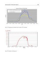
Fig. 4. Extrinsic mutual information transfer (EXIT) chart of used LDPC code 1024 bit length
constructed with edge distributions from Richardson et al. (2001).
4. Proposed receiver structure
4.1 Conditioned a posteriori decision-feedback
Following the decision-feedback strategy of Eq. (17) the estimator has no information about
the certainty of the feedback. Using soft-decision feedback the estimated sent vectors still
contain the noise from detection stage. The developing of the channel estimation error ε
[n]
can be very roughly modeled as follows:
ε
[n]=
σ
2
e
n
+ N
e

σ
2
c
(19)
On one hand the channel estimation error decreases with growing n through the averaging
effect, where the error energy per gained channel estimate sample due to noise and spatial
interference is denoted σ
2
e
. On the other hand an incorrect decision directly adds the error
energy σ
2
c
, which contains the energy of a false channel estimate plus noise and interference.
The cost of incorrect decisions are unequally higher as the benefit of another correct sample
for averaging, especially for higher n. Hence an incorrect decision should be avoided even at
the price of low number of samples to average.
By utilizing channel decoder L
D2
information at the decision stage, the feedback of incorrect
decisions can be avoided. For time-invariant channels the weighting factor is set to ξ :
= 1.0
because an update via Eq. (15) and (16) is applied only if the codeword associated with the
MIMO-OFDM symbol is successfully decoded. For linear block codes this is indicated by the
syndrome vector
γ
[n]=A · y[n]. (20)
The parity check matrix is denoted A, the received codeword is
y
[n]=sgn{L

D2
[n]}. (21)
Note that Eq. (20) and (21) are evaluated in most LDPC decoder implementations as break
criterion for the iteration process. So, if the decoder signals
γ [n]
H
= 0, where ·
H
denotes
the Hamming distance, the sent vectors in Eq. (15) and (16) are substituted by
{˜s[k, n]}
K
k=1
= M
n
T
{Π{y[n]}}, (22)
246
Adaptive Filtering Applications
Adaptive MIMO Channel Estimation Utilizing Modern Channel Codes 9
using the property of the systematic linear block code which renders additional re-encoding
unnecessary. Because of the high codeword distance it is unlikely that the codeword y
[n]
contains undetected errors or being another valid codeword. However, this is a source of
the algorithm’s residual errors. In the case
γ [n]
H
= 0, no update is performed instead the
former channel estimate is assumed to be still valid:
˜

H
[n, k] :=
˜
H
[n − 1, k], (23)
which can be seen as a simple zero order hold prediction.
As pointed out with the rough model in Eq. (19), feedback of erroneous data increases the
estimation error over-proportional compared to the benefit of another sample to average.
However, for valid codewords this approach leads to an extension of the training length due
to the usage of data symbols as virtual pilots. The benefit is especially large at the beginning
of a frame, directly after the end of pilots. There, the channel estimate error is still high and
therefore the probability of false detection is high. The proposed scheme is referred in the
following as Conditional Feedback (RLSCF).
The estimated channel matrix
˜
H is used in the MIMO detection, where LLR channel values
L
D1
are determined per OFDM symbol and subcarrier on a Maximum Likelihood (ML) basis:
L
D1
(t, ν)=
1
σ
2
w

min
s∈S
ν,+1

r −Hs− min
s∈S
ν,−1
r −Hs

, (24)
where
S
ν,+1
denotes the set of all possible send vectors that ν-th bit is +1, |S| = |M|
n
T
and
considering unit-power constellations. Of course, ML-approximating detection algorithms,
i. e. List Sphere Decoder (Hochwald & ten Brink, 2003) can be applied here as well. σ
2
w
is the
channel noise power which is often assumed to be known at the receiver.
4.2 Complexity discussion
Most of the proposed processing is straight-forward: OFDM demodulation, subcarrierwise
MIMO detection, de-interleaving and LDPC decoding has to be done in any coherent
MIMO receiver coping with multipath channels. The additional complexity comes from an
interleaver and a MIMO symbol mapper in the channel estimation feedback chain. In the
soft decision case there is more computing power necessary with only marginal performance
gains compared to the hard decision technique. However, the main contribution to complexity
raises in the channel estimation itself for possibly updating the channel estimation at each
OFDM symbol if the SNR is sufficient high and the channel decoder is successful decoding
the codeword. In this case the LDPC decoder that is aware of a valid codeword and stops the
iteration, needs less internal iterations so there is a shift in complexity from the decoder to the

channel estimator.
The estimation procedure can be further simplified by help of the matrix inversion lemma to
avoid explicit inversion of the autocorrelation matrix. The resulting algorithm is described in
Beinschob et al. (2009).
5. Numerical experiments
5.1 Channel estimation accuracy & system performance
In a MIMO system, the detection depends on the received vector r and channel matrix H
(Hochwald & ten Brink, 2003). In real scenarios the channel matrix is not available and an
247
Adaptive MIMO Channel Estimation Utilizing Modern Channel Codes
10 Will-be-set-by-IN-TECH
0
0.2
0.4
0.6
0.8
1.0
-6 0 6 12 18 24
avg. mutual information I
SNR in dB
■
■
■
■
■
■
■
■
■
■

■
●
●
●
●
●
●
●
●
●
●
●
▲
▲
▲
▲
▲
▲
▲
▲
▲
▲
▲
◆
◆
◆
◆
◆
◆
◆

◆
◆
◆
◆
★
★
★
★
★
★
★
★
★
★
★
▼
▼
▼
▼
▼
▼
▼
▼
▼
▼
▼
NMSE
■■
−30 dB
●●

−20 dB
▲▲
−10 dB
◆◆
−6dB
★★
−3dB
▼▼
0dB
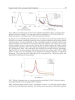
Fig. 5. Average Mutual Information of a MIMO 4 ×4 Spatial Multiplexing with 4-QAM
modulation and different levels of Channel Estimation Errors in terms of NMSE.
estimate
˜
H is used instead. To evaluate the quality of the detector output, which is of most
importance for the decision-directed scheme, the mutual information of the gained (uncoded)
LLRs is used (ten Brink, 1999). The performance degradation in presence of estimation errors
is assessed by modelling a channel estimate as follows:
˜
H
= H + ΔH, (25)
where H
r,t
∈CN(0, 1) are the i.i.d. MIMO Rayleigh Fading channel coefficients and elements
of ΔH are i.i.d. circular symmetric complex Gaussian random variables with error variance
σ
2
e
. This also covers to some extent the case of mobility induced interference because the ICI
leads to additional noise in the Frequency Domain as pointed out by Russell & Stuber (1995).
As a measure for the estimation error the normalized mean squared error is defined as

NMSE
=
n
T
∑
t=1
n
R
∑
r=1


H
r,t
−
˜
H
r,t


2
n
T
∑
t=1
n
R
∑
r=1
|

H
r,t
|
2
. (26)
So, the channel capacity for discrete input alphabet (4-QAM) and continuous channel output
isshowninFig.5.
In general, the capacity increases with SNR and with decreasing channel estimation NMSE.
However, a saturation of I over SNR can be observed: With increasing estimation error the
maximum level of mutual information I decreases.
At minimum, a NMSE of
−6dBto−10 dB is necessary for a half-rate coded system to work
properly. Below
−20 dB NMSE there is no significant difference in the system’s performance
using either the channel estimate or the actual channel matrix.
5.2 System le vel simulations for time-invariant channels
In Tab. 1 the system parameters are given for the experiments described in this section. For the
248
Adaptive Filtering Applications
Adaptive MIMO Channel Estimation Utilizing Modern Channel Codes 11
n
T
×n
R
4×4
Detector Maximum Likelihood
OFDM Subcarriers 128
Modulation 4-QAM
MIMO-OFDM symbols per frame 516
bandwidth efficiency

≈3.8 bit/s/Hz
Pilot symbols per antenna 4 (0.8%)
Channel Model
CN(0, 1)
channel multi-path order L 6
OFDM cyclic prefix L
cp
7
channel coherence time T
c
> frame length
LDPC code design rate R
c
1/2
codeword & interleaver length 1024 bit
Table 1. Simulation parameters for time-invariant channel
-20
-10
0
-1012345
NMSE in dB
E
b
/N
0
in dB
■
■
■
■

■
■
■
●
●
●
●
●
●
●
▲
▲
▲
▲
▲
▲
▲
◆
◆
◆
◆
◆
■■
LS
●●
RLS
▲▲
RLSsd
◆◆
RLSCF

10
-6
10
-5
10
-4
10
-3
10
-2
10
-1
10
0
-1012345
BER
E
b
/N
0
in dB
■
■
■
■
■
■
■
■
■

●
●
●
●
●
●
●
●
●
▲
▲
▲
▲
▲
▲
▲
▲
▲
◆
◆
◆
◆
◆
◆
◆
◆
★
★
★
★

■■
LS
●●
RLS
▲▲
RLSsd
◆◆
RLSCF
★★
PCSI
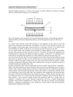
Fig. 6. BER and NMSE for the discussed schemes evaluated by Monte Carlo simulations
using time-invariant channels with system parameters defined in Tab. 1.
BER/NMSE system level simulations a Maximum Likelihood bit detector with LLR output,
combined with a short LDPC code of 1024 bit length, inserted in an MIMO-OFDM symbol,
were used. Simulations were conducted for the case of minimum pilot symbol length N
P
=
n
T
. The proposed channel estimation (RLSCF) was compared to the ordinary LS approach,
the hard/soft-decision feedback approach by Eq. (17) (RLS resp. RLSsd) and detection with
perfect channel state information (PCSI). Independent block-fading MIMO channel realization
were generated which were frequency-selective but time-invariant during the frame, see Eq.
(5).
The channel estimation error is assessed in terms of normalized mean squared error (NMSE),
shown in Fig. 6. Least Squares channel estimation using only the available short training
symbol sequence was inferior to the discussed decision-directed schemes. An improvement
of RLS/RLSsd over LS can be observed. With increasing E
b
/N

0
more correct feedback was
available and decreased the NMSE, as reflected by the stronger slope of the RLS/RLSsd curve.
RLS and RLSsd performed equally on average. The proposed method, RLSCF, performed
worse than RLS/RLSsd for low E
b
/N
0
. This is because the feedback is limited to valid
codewords only, which occurred seldom. So the averaging effect is almost as limited as in
249
Adaptive MIMO Channel Estimation Utilizing Modern Channel Codes
12 Will-be-set-by-IN-TECH
10
-2
10
-1
10
0
0 102030405060
˜
P
(γ 
H
= 0)
MIMO-OFDM symbol (codeword) n
0.0 dB
0.8 dB
1.6 dB
2.4 dB

(a) Rate of successful decoding as indicated by
γ 
H
= 0, for different channel E
b
/N
0
,comparing
proposed RLSCF (solid) and RLS (dashed lines).
-20
-10
0
0 102030405060
NMSE in dB
MIMO-OFDM symbol n
−0.8 dB
0.0 dB
0.8 dB
1.6 dB
2.4 dB
3.2 dB
(b) NMSE per MIMO-OFDM symbol (time) index
n and selected E
b
/N
0
.
Fig. 7. Developing of NMSE over time resp. OFDM symbol index for RLSCF scheme
(multiple frames and channel realizations averaged).
the LS case. Beyond 1 dB E

b
/N
0
RLSCF performed better than RLS/RLSsd because it can be
deduced that there were plenty of virtual pilots, as depicted in Fig. 7(a).
There the rate of indicated successful decoding over MIMO-OFDM symbol index n is shown.
Especially in the beginning of the frame a higher rate of successful decoding could be achieved
with the proposed channel estimator RLSCF. This led to more virtual pilots and improved
NMSE depicted in Fig. 7(b).
The developing channel estimation error in terms of normalized mean square error (NMSE)
can be seen for different E
b
/N
0
in Fig. 7(b). Due to the short training the channel estimation
error is rather high at the beginning of the frame and decreases with ∝ 1/n if the SNR is
sufficient so that the decoder could deliver successful decoded feedback. This the case for
E
b
/N
0
above ≈1 dB, below only insignificant improvements could be realized. This threshold
is a property of the LDPC code, which is visualized in the EXIT chart in Fig. 4. Only if the
input information exceeds the threshold successful decoding is possible. This means for the
proposed scheme, for E
b
/N
0
< 1 dB only marginal gains could to realized compared to LS,
where as for higher values significant improvements in terms of NMSE were achieved.

For completeness the resultant system Bit Error Rate (BER) of the conducted simulations are
shown in Fig. 6. For reference a curve for detection with perfect channel state information
(PCSI) is shown, too. On the right hand side the detection based on Least Squares channel
estimation using only the available training symbols is shown. The performances of the
discussed decision-directed schemes were in between, reflecting the same tendency as the
NMSE plot in Fig. 6. Here for higher E
b
/N
0
RLSsd performed marginal superior. By using
detection-based decision-directed strategies it was possible to decrease the BER but due to
erroneous feedback it was rather small. For the proposed conditional a-posteriori feedback
(RLSCF) a gain of 1 dB could be achieved. The gap of 2 dB to the decoding with perfect channel
knowledge can be explained with the limited codeword distance of the short LDPC code used.
250
Adaptive Filtering Applications
Adaptive MIMO Channel Estimation Utilizing Modern Channel Codes 13
-20
-10
0
0 40 80 120 160 200
NMSE in dB
MIMO-OFDM symbol n
−1dB
0dB
1dB
2dB
3dB
(a) ξ = 1.0
-20

-10
0
0 40 80 120 160 200
NMSE in dB
MIMO-OFDM symbol n
−1dB
0dB
1dB
2dB
3dB
(b) ξ = 0.9
-20
-10
0
0 40 80 120 160 200
NMSE in dB
MIMO-OFDM symbol n
−1dB
0dB
1dB
2dB
3dB
(c) ξ = 0.7
samples
ξ
10
0
10
1
10

2
0.7 0.8 0.9 1.0
(d) Eff. data window length
Fig. 8. Comparison of adaptivity on time variant channels (10 m/s) of channel code
constraint feedback (RLSCF) for different forgetting factors ξ, also shown the effective data
window length of forgetting factor in samples for coherence time (3 dB - blue line) and 10 dB
(red line).
5.3 Simulations for 3GPP channels
To evaluate algorithms for real application a realistic channel model is needed. In particular
the mobility component for the multipath MIMO case must be modelled very well. For this
purpose the 3GPP Spatial Channel Model (Spatial channel model for Multiple Input Multiple
Output (MIMO) simulations, 2008) is applied here.
5.3.1 Time adaptivity analysis
Fig. 8 illustrates the adaptivity of the DDCE structure depicted in Fig. 3. Clearly visible is the
balance of the forgetting factor ξ which was too inflexible if set to ξ
= 1.0 then the algorithm
failed to track the channel well, although the NMSE became very low after 60 symbols. On
the other hand, if set to ξ
= 0.7, even for 3 dB E
b
/N
0
the NMSE was insufficient for reliable
transmissions. So a higher E
b
/N
0
is needed for lower forgetting factors and thus higher
adaptivity to achieve the same system performance for mobility scenarios.
5.3.2 System level results

For the 3GPP channel simulations RLSCF-based DDCE schemes were investigated through
Monte Carlo simulations due to the lack of analytical tools to this kind of detection
and channel estimation feedback structure. A Point-to-Point link is considered with
Signal-to-noise-based assessment instead of range-dependence. Independent channel
realization were generated for each frame. A frame consisted of 516 MIMO-OFDM symbols
251
Adaptive MIMO Channel Estimation Utilizing Modern Channel Codes
14 Will-be-set-by-IN-TECH
10
-4
10
-3
10
-2
10
-1
10
0
-101234567
bit error rate
E
b
/N
0
in dB
■
■
■
■
■

■
■
■
■
■
■
●
●
●
●
●
●
●
●
●
●
●
▲▲
▲
▲
▲
▲
▲
▲
▲
▲
▲
◆
◆◆◆◆
◆

◆
◆
◆
◆
◆
◆
◆
◆
◆
■■
3m/s
●●
10 m/s
▲▲
30 m/s
◆◆
100 m/s
-20
-10
0
10
-101234567
NMSE in dB
E
b
/N
0
in dB
■
■

■
■
■
■
■
■
■
■
■
■
■
■
●
●
●
●
●
●
●
●
●
●
●
●
●
▲
▲
▲
▲
▲

▲
▲
▲
▲
▲
▲
▲
▲
◆
◆
◆
◆
◆
◆
◆
◆
◆
◆
◆
◆
◆
◆
◆
◆
◆
(a) RLS forgetting factor ξ = 0.9
10
-4
10
-3

10
-2
10
-1
10
0
-101234567
bit error rate
E
b
/N
0
in dB
■■■
■
■
■
●●●
●
●
●
●
▲▲▲
▲
▲
▲
◆
◆◆
◆
◆

◆
◆
■■
3m/s
●●
10 m/s
▲▲
30 m/s
◆◆
100 m/s
-20
-10
0
10
-101234567
NMSE in dB
E
b
/N
0
in dB
■
■
■
■
■
■
■
■
●

●
●
●
●
●
●
●
▲
▲
▲
▲
▲
▲
▲
▲
◆
◆
◆
◆
◆
◆
◆
◆
(b) RLS forgetting factor ξ = 0.7
Fig. 9. On the left BER vs. E
b
/N
0
for burst transmissions in time variant channels with
minimal pilot length N

P
= n
T
for 4 ×4 MIMO, on the right channel estimation error in
NMSE (same legend as left hand).
constructed by modulating uncorrelated random bits. Transmissions were simulated until
either 3
×10
5
bit were transmitted or at least 200 frames errors were encountered per E
b
/N
0
and velocity setting. The E
b
/N
0
level was not further increased if in 3 ×10
5
bit no bit errors
occurred after the channel decoder.
As seen from the results for time-invariant channels, RLSCF clearly gave best results in terms
of BER/NMSE. As already mentioned, in order to maximize the bandwidth efficiency, we
focus on having minimal number of pilot symbols, that is when N
P
= n
T
.Soforthe4× 4
MIMO system we employed 4 pilot tones per subcarrier and spatial stream, having a pilot
rate of 0.8 %.

As pointed out in the previous section, it is obvious that the forgetting factor has influence on
the NMSE performance due to the averaging effect. Left of Fig. 9 shows the BER of RLSCF for
increasing velocities of the mobile terminal. But it is difficult to predict whether an improved
adaptivity on time-variant channels pays off the lost samples for the averaging. Simulation
results for comparative study can be seen in Fig. 9. For a forgetting factor of ξ
= 0.9 (see
252
Adaptive Filtering Applications
Adaptive MIMO Channel Estimation Utilizing Modern Channel Codes 15
Fig. 9(a)), it can be seen that performance degradation started somewhere above 30 m/s. For
lower velocities virtually error-free reception was observed for E
b
/N
0
above 4.5 dB. In the case
of very high velocities, strong variations in the channel occurred which led to an increased
channel estimation error in terms of NMSE.
In comparison with the forgetting factor setting of ξ
= 0.7 (see Fig. 9(b)), we observed a
general rise in NMSE due to the smaller effective data window length, which in turn leads to a
worse BER. An exception is the highest velocity, which seemed unaffected by the shorter data
window size in terms of NMSE. The same NMSE performance for ξ
= 0.7 and ξ = 0.9 could
be achieved. We can deduce that for 100 m/s during the longer data window size the channel
changed significantly and therefore the additional samples were of no use for the averaging
process. While the NMSE seemed unaffected there was influence visible in the BER results. A
shorter window length led to a earlier E
b
/N
0

level of virtually error-free transmission, about
1 dB.
6. Conclusion
A promising structure to perform channel estimation for a multitude of channel scenarios
using minimum amount of pilots enhanced by decision-directed techniques is presented.
Through the employment of modern channel coding in the feedback the algorithm is capable
to improve the channel estimate thus decreasing the estimation error beyond the pilot
sequence only by using data symbols as virtual pilots. Optimal tracking of time-variant
channels is still an open problem, although good results can be achieved by regarding
influence length resp. coherence time of the channel and choosing the forgetting factor ξ
appropriately. However, in many practical cases lower velocities are encountered which can
be exploited quite well with a high forgetting factor like ξ
= 0.9 as shown in the results. For
highest velocities we loose about 1 dB in E
b
/N
0
butgaininNMSEandBERforthelower
velocities. There is a general trade-off between good system performance in low E
b
/N
0
or
high velocities scenarios where the usable data window size gets too small for significant
averaging gains in the channel estimation.
7. References
Akhtman, J. & Hanzo, L. (2007a). Advanced channel estimation for MIMO-OFDM in
realistic channel conditions, IEEE International Conference on Communications, ICC ’07
pp. 2528–2533.
Akhtman, J. & Hanzo, L. (2007b). Iterative receiver architectures for MIMO-OFDM, IEEE

Wireless Communications and Networking Conference, WCNC, pp. 825–829.
Beinschob, P., Lieberei, M. & Zölzer, U. (2009). An error propagation prevention method for
MIMO-OFDM RLS-DDCE algorithms, Proc. IEEE International Symposium On Wireless
Communication Systems 2009 (ISWCS’09), Siena pp. 31–35.
Beinschob, P. & Zölzer, U. (2010a). Improving Low-Delay MIMO-OFDM channel estimation,
International ITG Workshop on Smart Antennas 2010,Bremen,Germany.
Beinschob, P. & Zölzer, U. (2010b). MIMO-OFDM equaliser for spatial multiplexing
transmission modes, Advances in Radio Science 8: 81–85.
URL: />Bölcskei, H., Gesbert, D. & Paulraj, A. (2002). On the capacity of OFDM-based spatial
multiplexing systems, IEEE Transactions on Communications 50(2): 225–234.
253
Adaptive MIMO Channel Estimation Utilizing Modern Channel Codes
16 Will-be-set-by-IN-TECH
Chu, D. C. (1972). Polyphase codes with good periodic correlation properties, IEEE
Transactions on Information Theory 18(4): 531–532.
Dall’Anese, E., Assalini, A. & Pupolin, S. (2009). On the effect of imperfect channel
estimation upon the capacity of correlated MIMO fading channels, IEEE 69th
Vehicular Technology Conference, VTC Spring 2009, pp. 1–5.
Gallager, R. G. (1962). Low-density parity-check codes, IRE Transaction on Information Theory
8(1): 21–28.
Gallager, R. G. (1963). Low Density Parity-Check Codes, MIT Press, Cambridge, MA.
Glavieux, A., Loat, C. & Labat, J. (1997). Turbo equalization over a frequency selective channel,
Proceedings of the International Symposium of Turbo Codes, Brest, France pp. 96–102.
Hagenauer, J., Offer, E. & Papke, L. (1996). Iterative decoding of binary block and
convolutional codes, IEEE Transactions on Information Theory 42(2): 429–445.
Hochwald, B. & ten Brink, S. (2003). Achieving near-capacity on a multiple-antenna channel,
IEEE Transactions on Communications 51(3): 389–399.
Liu, H., Wang, X. & Xiong, Z. (2003). Iterative receivers for OFDM coded broadband MIMO
fading channels, IEEE Workshop on Statistical Signal Processing pp. 355–358.
Lozano, A. & Jindal, N. (2010). Transmit diversity vs. spatial multiplexing in modern MIMO

systems, IEEE Transactions on Wireless Communications 9(1): 186–197.
MacKay, D. (1999). Good error-correcting codes based on very sparse matrices, IEEE
Transactions on Information Theory 45(2): 399–431.
Proakis, J. G. & Salehi, M. (1994). Communication Systems Engineering,PrenticeHall
International, Eaglewood Cliffs, New Jersey 07632.
Richardson, T. J., Shokrollahi, M. A. & Urbanke, R. L. (2001). Design of capacity-approaching
irregular low-density parity-check codes, IEEE Transactions on Information Theory
47(2): 619–637.
Russell, M. & Stuber, G. (1995). Interchannel interference analysis of OFDM in a mobile
environment, IEEE 45th Vehicular Technology Conference, VTC 1995, Vol. 2, pp. 820–824.
Spatial channel model for Multiple Input Multiple Output (MIMO) simulations (2008). Technical
Report 25.996, 3rd Generation Partnership Project (3GPP), Technical Specification
Group Radio Access Network, 06921 Sophia-Antipolis Cedex, France.
ten Brink, S. (1999). Convergence of iterative decoding, Electronics Letters 35(10): 806–808.
ten Brink, S. (2001). Convergence behavior of iteratively decoded parallel concatenated codes,
IEEE Transactions on Communications 49(10): 1727–1737.
ten Brink, S., Kramer, G. & Ashikhmin, A. (2004). Design of low-density parity-check codes
for modulation and detection, IEEE Transactions on Communications 52(4): 670–678.
254
Adaptive Filtering Applications
12
An Introduction to ANFIS Based Channel
Equalizers for Mobile Cellular Channels
K. C. Raveendranathan
Government Engineering College Bartonhill Vanchiyoor P.O.
India
1. Introduction
The purpose of a communication system is to transfer information between two separate
points over some medium in the presence of disturbances or distortions such as noise and
dispersion. This distortion is manifested in the time domain as pulse dispersion and is

labeled as Inter-Symbol Interference (ISI). As data rates increase in modern digital
communication systems, ISI becomes an inevitable consequence of the dispersive nature of
band-limited propagation channels. The receiver must include an equalizer to mitigate the
effects of ISI. The function of the equalizer is to combat the ISI and to utilize the available
spectrum most efficiently.
Equalizers are cascaded to almost all kinds of channels, right from telephone lines to radio
and optical fiber channels, to make the channel performance optimal. Ideally, an equalizer,
when cascaded to the end of a channel, will make it behave like an ideal channel, the one
which will not distort the signals in any manner. In the case of mobile cellular channels,
which are generally considered to be Non-Linear and Time Variant (NLTV), the design of
equalizers is not a trivial problem. Moreover, the above said channel has certain uncertainties
in its behaviour, which need to be tackled in the equalizer design. The Co-Channel
Interference (CCI) due to frequency reuse and Adjacent Channel Interference (ACI) due to
spectral leakage, both contribute to the reduction in overall Signal-to-Interference-Noise-
Ratio (SINR) in mobile cellular channels.
In applications in which the Channel Impulse Response (CIR) is unknown and no training
sequence is available, the equalizer must be computed/ updated blindly from the received
signal and knowledge of the statistics of the data source alone. A common approach in
continuous transmission systems is to blindly update a Linear Equalizer (LE) using the
Constant Modulus Algorithm (CMA), and then switch to a Decision Directed (DD) mode
when the Symbol Error Rate (SER) is low enough (Widro, 1973).
2. Fading characteristics of mobile channels
In mobile cellular radio transmission between a base station and a mobile telephone, the
signal transmitted from the base station to the mobile receiver is usually reflected from
surrounding buildings, hills, and other obstructions. As a consequence, we observe multiple
propagation paths arriving at the receiver at different delays. Hence the received signal has
characteristics similar to those for ionospheric propagation. The same is true for