Adaptive Filtering Applications
202
contaminated SEP was set to −10, −15 and −20 dB. The last row of Figure 3 (sn) shows the
simulated primary channel SEP signal at -15dB with EEG and WGN.
2.3 Adaptive noise canceller for SEP extraction using mean square estimation
The SEP extraction method under the adaptive noise canceller (ANC) framework derived from
the Mean-Square-Error was firstly introduced and evaluated by some of the present authors in
(Lam et al., 2005). From the adaptive filter theory (Haykin, 2001) and the configuration of the
ANC shown in Figure 1, the SEP extraction problem can be solved as a linear ANC problem
since the FIR adaptive filter is used (named as ANC-SEP approach in this study). The
commonly used error measure is the Mean-Square-Error (MSE defined as J
MSE
=E[e
2
(n)], where
E[.] represents the ensemble operator). The minimisation of the MSE results in the Wiener
normal equation under some statistically independent and signal wide-sense stationary (WSS)
assumptions. The optimal solution of Wiener normal equation can be denoted as:

-1
() () ()
opt mse mse
nnnwRP (3)
where
P
mse
is the cross-correlation vector between s(n) and r n , and R
mse
is the

autocorrelation matrix of
r(n), which can be written as

[( )( )]
mse
Esn nPr

[() ()]
T
mse
Ek kRrr (4)
As discussed in many literatures, the well-known least mean squares (LMS) algorithm is a
stochastic gradient based adaptive algorithm to obtain the optimal solution of J
MSE
. The
updating of the adaptive filter coefficient vector can be denoted as (Haykin, 2001)

() ( 1) 2 ()()
lms
nn enn


ww r (4)
where

lms
is the stepsize which is one of the most important factors that controls the initial
convergence rate and steady state error of the LMS-ANC for SEP extraction. Generally, a big
stepsize yields rapid convergence but larger steady-state misadjustment error. A small
stepsize yields slow convergence but a corresponding smaller steady-state misadjustment

error. There exists a theoretical lower and upper bound of the choice of

lms
(details can be
referred to (Haykin, 2001). Usually, the choice of

lms
is suggested by the following condition
in the LMS algorithm (Haykin, 2001)

01/()
in
M
P


(5)
where P
in
and M is the input power and the order of the adaptive FIR filter, respectively. In
principle, the selection of the stepsize not only depends on the desired steady-state error
level but also the statistical properties of the input signal of the adaptive filter. In other
words, the convergence rate of the LMS algorithm is greatly affected by the dynamic range
of the eigenvalues of the autocorrelation matrix
R
mse
. Considering this essential limitation, it
is not difficult to understand that the performance of the ANC-SEP approach using LMS
algorithm may suffer from the conflict to the WSS assumption for s(n) and r(n) and the
nonstationary property of the r(n) .


Fast Extraction of Somatosensory Evoked Potential Based on Robust Adaptive Filtering
203
2.4 Adaptive noise canceller for SEP extraction using least square estimation
Motivated by the performance enhancement of the ANC-SEP method using LMS
algorithm compared with EA-SEP (Hu et al., 2005; Lam et al., 2005; Cui et al., 2008), some
investigations of the ANC-SEP using RLS algorithm have been carried out and presented
in (Ren et al., 2009). Instead of using MSE cost function, a conventional least square (LS)
cost function is employed and the optimal solution of J
LS
is described as follows (Haykin
2001)

2
1
() ()
n
nk
LS
k
Jn ek





, and
1
() () ()
opt Ls LS

nnn

wRP (6)
where,

is the forgetting factor with the value between 0 and 1, which controls the effective
amount of data used in the averaging and hence the degree to which the RLS algorithm can
track the signal variation. The closer the value of λ goes to one, the lower will be the steady-
state misadjustment error of the RLS algorithm. Its tracking ability, however, will also be
slower.
R
LS
(n) is the autocorrelation matrix of the input vector at time index n and P
LS
(n) is
the cross-correlation vector between the input vector and the reference signal at time index
n. Generally, they can be estimated as

n
ni T T
LS LS
i
niinnn





RrrRrr


(7)


n
ni
LS LS
i
nsiinsnn





P
rP r

(8)

By applying the matrix inversion lemma to the optimal solution in (6), the famous recursive
least square (RLS) algorithm can be derived, and it is summarized in Table 1 for the
completeness (Interested readers can refer to (Haykin, 2001)). From Table 1, it is noted that
the computational complexity of the RLS algorithm is of order M
2
.
1) Initialization: (1) 0
RLS

w ,
1
(1)

RLS M
n


PI, n=0, where M is the
filter order of the adaptive filter using in ANC,

can be the inverse of an
estimation of the input signal power.
2) Calculation of the adaptive filter output: ( ) ( ) ( 1)
T
RLS
yn n n

rw
3) Estimation error:
() () ()en sn yn


4) Calculation of the Kalman gain vector:
(1)()
()
() ( 1) ()
RLS
RLS
T
RLS
nn
n
nn n







Pr
K
rP r

5) Update of the inverse correlation matrix:

1
() ( 1) () () ( 1)
T
RLS RLS RLS RLS
nn nnn



 


PPKrP

6) Update of the filter weights:
() ( 1) ()()
RLS RLS RLS
nn nenww K
n=n+1, back to step 2)

Table 1. RLS-ANC-SEP algorithm

Adaptive Filtering Applications
204
2.5 Adaptive noise canceller for SEP extraction using robust estimation
Carefully evaluating the properties of the recording SEP signals in the operating room, it
noted that these SEP signals may have some nonstationary and impulsive like properties
when the trial patients happen to the eye movement, cough and stimulus etc, which
commonly exist. Under these kind of circumstances, the performance of the ANC-SEP
methods using LMS or RLS will degrade or fail to extract SEP signal due to the adverse
effect of the noise. The new method is desired. Motivated by the research work done by
Chan and Zou (Chan & Zou, 2004), a new error measure method based on the M-estimate
has been introduced and the corresponding cost function instead of J
MSE
or J
LS
is used for
providing the robustness in the algorithm, which is given as




11
() () () ()()
nn
ni ni T
R
ii
J n ei si n i
 





wr (10)
where

is the positive forgetting factor and

is an M-estimate function, which provides
certain ability to suppress the adverse effect of impulsive noise on the cost function when
the error signal becomes very large. In our study, the Huber M-estimate function and the
related weighting function are used, which can be denoted as

ee
e
otherwise










(11)

where


is the threshold parameter. The optimal solution w(n) for minimizing J
R
(n) can be
obtained by differentiating (10) with respect to
w(n) and setting the derivatives to zero. This
yields the following M-estimate normal equation

() () ()
RR
nn n

Rw P (12)
where
() ( 1) (())() ()
T
RR
nn
q
en n n

RR rr (13)

() ( 1) (())()()
RR
nnqensnn


PP r (14)


1, 0
()/
()
0,
e
de de
qe
otherwise
e










(15)
where,
R
R
(n) and P
R
(n) are called the M-estimate correlation matrix of r(n) and the M-
estimate cross-correlation vector of
r(n) and s(n), respectively. The adaptive algorithm for
solving the normal equation (12) can be obtained in the same way as developing RLS
algorithm, and the resulting algorithm is called recursive least M-estimate algorithm (RLM)

and it is summarized in Table 2. From Table 1 and Table 2, it can be seen that the
computational complexity of RLM and RLS is similar except the cost to determine the
weighting function q(e) in (15). It is also noted that when the signal is Gaussian distributed,
RLS and RLM are identical. The contribution of the weight function q(e(n)) lies at the
suppression of the adverse effects of the large estimation error due to the undesired
impulsive interference on the adaptive filter weight vector
w(n). The degree of this
suppression is controlled by the parameter

in our study, a recursive estimation approach

Fast Extraction of Somatosensory Evoked Potential Based on Robust Adaptive Filtering
205
is adopted which directly connects to the variance of the estimation error under the
assumption of the interference is with contaminated Gaussian (CG) or alpha-stable
distributions. The parameter

has been determined (shown in Table 2) when there is 95%
confidence to detect and reject the impulses (Chan & Zou, 2004).
1) Initialization: (1) 0
RLM

w ,
1
(1)
RLM M
n


PI, n=0, where M is the filter

order of the ANC,

can be the inverse of an estimation of the input signal
power.
2) Calculation of the adaptive filter output: ( ) ( ) ( 1)
T
RLM
yn n n

rw
3) Estimation error calculation:
() () ()en sn yn


4) Estimate the variance of the estimation error, determine the parameter
 and
determine the weighting function (Chan & Zou, 2004)
：


22
1
() ( 1) (1 ) ()
e
nn cmedAn

 
 , 2.24 ( )n




,
1, 0
()
0,
e
qe
otherwise









，

where


is the forgetting factor,
22
() { (), , ( 1)}
ew
An en enN ,
w
N is the
length of the estimation window, and

1
1.483(1 5 /( 1))
w
cN

 is the finite
sample correction factor
5)Calculation of the Kalman gain vector:
(( )) ( 1)( )
()
(( )) ( ) ( 1)( )
RLM
R
T
RLM
qen n n
n
qen n n n




Pr
K
rP r

6) Update of the inverse correlation matrix:

1
() ( 1) () () ( 1)

T
RLM RLM RLM RLM
nn nnn



 


PPKrP

7) Update of the filter weights:
() ( 1) ()()
RLM RLM R
nn nenww K
8) Calculate the estimation error:
(), () 1
()
(1),()0
en qe
en
en qe









n=n+1, back to step 2)

Table 2. RLM algorithm
3. Simulation study and discussion
As discussed above, we have introduced the SEP extraction approaches under the ANC
framework by using different adaptive filtering algorithms. Specifically, employing LMS,
RLS and RLM algorithms to update the weighting vector of the adaptive FIR filter in ANC
results in the LMS-ANC-SEP method, RLS-ANC-SEP method and RLM-ANC-SEP method,
respectively. In this section, the performance of these adaptive filtering methods for SEP
extraction under Gaussian and impulsive noise environment has been evaluated and
compared by intensive simulation experiments.
3.1 Experiment 1: SEP extraction under Gaussian noise
In this section, we aim to visually illustrate the SEP extraction performance of the
algorithms discussed above under Gaussian noise condition. The detailed performance

Adaptive Filtering Applications
206
comparison between EA-SEP, LMS-ANC-SEP, RLS-ANC-SEP and RLM-ANC-SEP methods
under EEG and WGN contamination can be referred to the work presented in papers (Lam
et al., 2005) and (Ren et al., 2009). Here, we only illustrate one set of the SEP extraction
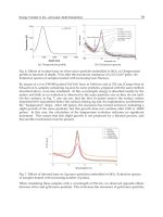
results for reader’s favorite review. Figure 4 shows the SEP extraction results from 50 SEP
trails by different algorithms. In this experiment, the SEP template (xn), simulated primary
signals (sn, vn) and reference signal (rn) are the same as those shown in Figure 3 at SNR=-
15dB. The order of the adaptive filter M is set to be 10, the step size μ of the LMS-ANC-SEP
is chosen as 2x10
-4
, the forgetting factor of the RLS-ANC-SEP and RLM-ANC-SEP algorithms
is set to be 0.99. The parameters for RLM-ANC-SEP in Table 2 are set as



=0.9 and N
w
=7.
From Figure 4, it is clear to see that the signals extracted from 50 trials by EA-SEP and LMS-
ANC-SEP are difficult to detect the positive and negative peaks required for quantitative
analysis and diagnosis of the SEP signal. More precisely, the positive peak around 35ms and
the negative peak around 40ms, which are two most commonly-used criteria for the online
monitoring during the spinal surgery, are still buried in the heavy background noise, so that
their latencies and amplitudes cannot be measured accurately. On the other hand, we can
see that the performance of RLM-ANC-SEP is almost the same as that of RLS-ANC-SEP,
which outperforms than other two algorithms. It is apparent that two peaks around 35ms
and 40 ms can be easily observed and their latencies and amplitudes can be precisely
measured in the results using RLS-ANC-SEP and RLM-ANC-SEP methods. All these
findings in practice can be well explained in theory. That is, the RLS/RLM-based algorithms
have a fast convergence rate than LMS-based algorithm. Furthermore, the RLM-ANC-SEP
algorithm is comparable to RLS-ANC-SEP algorithm under EEG and WGN environment. We
next test and compare their performances when few SEP trials are contaminated with
impulsive noises.
0 20 40 60 80 100
-2
-1
0
1
2
SEP extraction at SNR=-15dB 50 trials under WGN
EA-SEP
ms
0 20 40 60 80 100
-2
-1

0
1
2
LMS-SEP
ms
0 20 40 60 80 100
-2
-1
0
1
2
RLS-SEP
ms
0 20 40 60 80 100
-2
-1
0
1
2
RLM-SEP
ms

Fig. 4. 50-trial SEP extraction results obtained by EA-SEP, LMS-ANC-SEP, RLS-ANC-SEP,
and RLM-ANC-SEP method, respectively (SNR=-15dB)

Fast Extraction of Somatosensory Evoked Potential Based on Robust Adaptive Filtering
207
3.2 Experiment 2: SEP extraction under impulsive noise
This simulation is set up to compare the SEP extraction performance of the EA-SEP, LMS-
ANC-SEP, RLS-ANC-SEP and RLM-ANC-SEP under EEG and individual impulse

contaminated noise environment. Generally, the impulsive noise can be generated by a
contaminated Gaussian (CG) model proposed in (Haweel & Clarkson, 1992). The impulses
are generated individually with arrival probability P
ar
=2×10
-3
and the variance is chosen as 200. In
our study, only for performance illustration purpose, the positions of the impulses are assumed to
occur at 19ms, 28ms, 35ms, 44ms, and 78ms, respectively (which is not necessary to fix the
position of the impulses, but here it is for us to gain the better performance visualization for
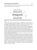
different algorithms). The SEP template (xn), one sample primary interference (vn) with
impulses, one sample of the reference signal (rn) and the resultant primary signal (sn) at -15dB
are shown in Figure 5. The difference between Figure 3 and Figure 5 only lies at several impulses
added in the primary interference signal (vn). In this case, the primary signal is composed of a SEP
template, an A1-Fz EEG component, and a contaminated Gaussian noise.

0 20 40 60 80 100
-2
-1
0
1
2
xn
ms
0 20 40 60 80 100
-10
-5
0
5
10

vn
ms
0 20 40 60 80 100
-10
-5
0
5
10
rn
ms
0 20 40 60 80 100
-10
-5
0
5
10
sn
ms

Fig. 5. SEP signals with impulsive noise, (1) xn and rn are the same as those in Figure 3. (2)
vn: one example of recorded A1-Fz used as EEG tegether with CG noise for primary
channel; (3) sn: One example of the primary channel signal (EEG +SEP+CGN) at -15 dB.
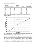
For this simulation, all parameter settings are the same as those used in Experiment 1. The
SEP extraction results from 50 SEP trails under impulsive noise by different algorithms are
shown in Figure 6. If no impulsive noise occurs, the extraction results of four different methods
should be approximately identical to their counterparts in Figure 4. As a result, Figure 5 can be
regarded as a standard to evaluate the robustness of these methods when impulsive noises are
added. From Figure 6, it is clear to see that the adverse impact of the impulses on the SEP
extraction for EA-SEP, LMS-ANC-SEP and RLS-ANC-SEP algorithms compared with their
counterpart algorithms under WGN shown in Figure 4. More specifically, for the EA-SEP


Adaptive Filtering Applications
208
method, since the amplitudes of the impulsive noise are rather large compared to that of
WGN, they cannot be averaged out completely using finite number of trials. As for the LMS-
ANC-SEP and RLS-ANC-SEP methods, which employ an LS criterion for the updating of the
filter coefficients in ANC, their performances are degraded severely because the coefficient
estimates in ANC are unstable and may be greatly deviated from the reasonable values
when impulsive noise occurs. The performance degradation can be more easily observed in
the result of RLS-ANC-SEP in Figure 6, where the adverse impacts of impulsive noises
around 35ms and 44ms are distinct and its difference with RLS-ANC-SEP of Figure 4 is
obvious. Unlike those methods based on averaging or LS criterion, RLM-ANC-SEP employs
an M-estimation function in ANC so that the impulsive noise can be detected and
suppressed effectively. As the result, its harmful impact on SEP extraction is reduced
considerably. The simulation results illustrate the advantage of RLM-ANC-SEP, and we can
see that RLM-ANC-SEP shows its robustness to the impulsive interferences and its
performance is close to that under WGN condition. In Figure 6, we can hardly find the traces
of impulsive noise in the RLM-ANC-SEP result and peaks were clearly seen and measurable.
In a simple word, impulsive noise which degrades the outputs of EA-SEP, LMS-ANC-SEP
and other LS-based SEP extraction methods will do little harm to RLM-ANC-SEP.

0 20 40 60 80 100
-2
-1
0
1
2
SEP extraction at SNR=-15dB 50 trials under impulsive noise
EA-SEP
ms

0 20 40 60 80 100
-2
-1
0
1
2
LMS-SEP
ms
0 20 40 60 80 100
-2
-1
0
1
2
RLS-SEP
ms
0 20 40 60 80 100
-2
-1
0
1
2
RLM-SEP
ms

Fig. 6. 50-trial SEP extraction results obtained by EA-SEP, LMS-ANC-SEP, RLS-ANC-SEP,
and RLM-ANC-SEP method, respectively (SNR=-15dB)
As mentioned before, impulsive noise often occurs during spinal surgery in operating
theatres and it will greatly decrease the quality of SEP recording. Current SEP recording
technique works in this way when some SEP trials are contaminated with impulsive noise,

they will be discarded. However, these trials with impulsive noise also contain useful SEP
information, and the rejection of these trials will increase the time to record a useful SEP

Fast Extraction of Somatosensory Evoked Potential Based on Robust Adaptive Filtering
209
signal, and make the recording and monitoring discontinuous, which is undesirable.
Therefore, making use of SEP trials contaminated with impulsive noise is necessary and
robust SEP extraction method, such as the proposed RLM-ANC-SEP method, is
advantageous. Our preliminary study and experimental results show that the RLM-ANC-
SEP method has an excellent performance in impulsive noise environment, it may be taken
as a good solution to achieve reliable and continuous SEP recording for monitoring under
Gaussian and impulsive noise environment.
4. Conclusion
Aiming at developing the efficient SEP recording system, we have introduced the SEP
extraction methods under the ANC framework using adaptive FIR filter. A new SEP
extraction method called RLM-ANC-SEP was developed to obtain the the fast and robust
performance under Gaussian and Contaminated Gaussian noise environment. RLM-ANC-
SEP minimizes the modified Huber M-estimator based cost function instead of the
conventional mean square error and least squares error based cost functions, which
provides the robust ability when impulses occurring in the primary channel, and maintains
the fast convergence as the RLS-ANC-SEP algorithm. Simulation study proved that either
RLM-ANC-SEP or RLS-ANC-SEP has better and more robust convergence performance than
LMS-ANC-SEP. The performances of RLM-ANC-SEP and RLS-ANC-SEP showed equivalent
under WGN condition, but RLM-ANC-SEP presented its robustness to the impulsive
interferences. Clinical application and validation study could be our future work on this
proposed SEP signal extraction approach.
5. Acknowledgment
This work was partially supported by Shenzhen Science and Technology Program (No.
08CXY-01), Hong Kong ITF Tier 3 (ITS/149/08), and Research Grants Council of the Hong
Kong SAR (GRF HKU7130/06E).

6. References
Chan, S. C. & Y. X. Zou (2004). A Recursive Least M - Estimate Algorithm for Robust
Adaptive Filtering in Impulse Noise: Fast Algorithm and Convergence
Performance Analysis, IEEE Transactions on Signal Processing, Vol. 52, No.4, pp. 975-
991.
Cui, H., C. Shen, et al. (2008). Study on Adaptive Noise Canceller Based on Fixed-Point
Algorithm for Real-Time Somatosensory Evoked Potential Monitoring,
Bioinformatics and Biomedical Engineering, Vol. 3, pp.2213 – 2216.
El-Hawary, R., S. Sparagana, et al. (2006). Spinal Cord Monitoring in Patients with Spinal
Deformity and Neural Axis Abnormalities: A Comparison with Adolescent
Idiopathic Scoliosis Patients, SPINE, Vol. 31, No. 19, pp.E698-E706.
Etter, D. M. & S. D. Stearn (1981). Adaptive Estimation of Time Delays in Sampled Data
Systems, IEEE Transactions on Acoustic, Speech, Signal Processing, Vol. 29, pp. 582–
587.
Haweel, T. I. & P. M. Clarkson (1992). A Class of Order Statistic LMS Algorithms, IEEE
Transactions on Signal Processing, Vol. 40, No. 1, pp. 44-53.

Adaptive Filtering Applications
210
Haykin, S. (2001). Adpative Filter Theory (4th Edition), Prentice Hall.
Hazarika, N., A. Tsoi, et al. (1997). Nonlinear Considerations in EEG Signal Classification,
IEEE Transactions on Signal Processing, Vol. 45, pp. 829–836.
Hu, Y., B. Lam, et al. (2005). Adaptive Signal Enhancement of Somatosensory Evoked
Potential for Spinal Cord Compression Detection: An Experimental Study,
Computers in Biology and Medicine, Vol. 35, pp. 814-828.
Kong, X. & T. S. Qiu (1999). Adaptive Estimation of Latency Change in Evoked Potentials by
Direct Least Mean p-Norm Time-Delay Estimation, IEEE Transactions On Biomedical
Engineering, Vol. 46, No.8, pp. 994-1003.
Krieger, D. & R. Sclabassi (2001). Real-Time Intraoperative Neurophysiological Monitoring,
Methods, Vol. 25, pp. 272-287.

Lam, B., Y. Hu, et al. (2005). Multi-adaptive Filtering Technique for Surface Somatosensory
Evoked Potentials Processing, Medical Engineering & Physics, Vol. 27, pp. 257-266.
Lange, D. H. & G. F. Inbar (1996). A Robust Parametric Estimator for Single-Trial Movement
Related Brain Potentials, IEEE Transactions on Biomedical Engineering, Vol. 43, pp.
341-347.
Lin, B. S., B S. Lin, et al. (2004). Adaptive Interference Cancel Filter for Evoked Potential
Using High-Order Cumulants. IEEE Engineering in Medicine and Biology Society, Vol.
1, pp.396-398.
MacDonald, D. B. & A. Z. Zayed (2005). Tibial Somatosensory Evoked Potential
Intraoperative Monitoring: Recommendations Based on Signal to Noise Ratio
Analysis of Popliteal Fossa, Optimized P37, Standard P37, and P31 Potentials, Journal
of Clinical Neurophysiology, Vol. 116, No.8, pp. 1858-1869.
MacLennan, A. R. & D. F. Lovely (1995). Reduction of Evoked Potential Measurement Time
by a TMS320 Based Adaptive Matched Filter, Medical Engineering & Physics, Vol. 17,
pp. 248-256.
McGillem, C. & J. Aunon (1981). Signal Processing in Evoked Potential Research:
Applications of Filtering and Pattern Recognition, Critical Reviews in Bioengineering,
CRC, Vol. 9, pp. 225-265.
Nash, C. L., R. A. Lorig, et al. (1977). Spinal Cord Monitoring During Operative Treatment
of the Spine, Clinical Orthopaedics and Related Research, Vol. 126, pp. 100-105.
Nishida, S. & M. Nakamura (1993). Method for Single-Trial Recording of Somatosensory
Evoked Potentials, Journal of Biomedical Engineering, Vol. 15, pp. 257-262.
Ren, Z. L., Y. X. Zou, et al. (2009). Fast Extraction of Somatosensory Evoked Potential using
RLS Adaptive Filter Algorithms, The 2nd International Congress on Image and Signal
Processing (CISP'09), pp. 4444-4447.
Turner, S., P. Picton, et al. (2003). Extraction of Short-Latency Evoked Potentials Using a
combination of Wavelets and Evolutionary Algorithms, Medical Engineering &
Physics, Vol. 25, pp. 407-412.
Wei, Q. & K. Fung (2002). Adaptive Filtering of Evoked Potentials with Radial-Basis-
Function Neural Network Prefilter, IEEE Transactions on Biomedical Engineering,

Vol. 49, pp. 225-232.
Woody, C. D. (1967). Characterization of an Adaptive Filter for the Analysis of Variable
Latency Neuroelectric Signals, Medical Biology Engineering, Vol. 5, pp. 539-553.
Part 3
Communication Systems


10
A LEO Nano-Satellite Mission for the
Detection of Lightning VHF Sferics
Ghulam Jaffer
1,2
, Hans U. Eichelberger
2
,
Konrad Schwingenschuh
2
and Otto Koudelka
1

1
Institute of Communication Networks and Satellite Communications
Graz University of Technology, Graz
2
Space Research Institute, Austrian Academy of Sciences, Graz
Austria
1. Introduction

The LiNSAT is a proposed project for the detection of electromagnetic signatures produced
by lightning strokes (Sferics) in very high frequency (VHF) range in low-earth-orbit (LEO)

around 800 km. The satellite is 20 cm cube and weighs ~ 5 kg. The main scientific objective
of the planned LiNSAT is the investigation of impulsive electromagnetic signals generated
by electrical discharges in terrestrial thunderstorms (lightning), blizzards, volcanic
eruptions, earthquakes and dust devils. These electromagnetic phenomena called Sferics
cover the frequency range from a few Hertz (Schumann resonances) up to several GHz.
Depending on the source mechanism, the wave power peaks at different frequencies, e.g.
terrestrial lightning has a maximum power in the VLF and HF range, also trans-ionospheric
pulses reaching at LEO and possibly to satellites in geostationary-Earth-orbit (GEO) peak at
VHF. The global terrestrial lightning rate is in the order of 100 lightning flashes per second
with an average energy per flash of about 10
9
Joule (Rakov and Uman 2003). Only a small
percentage of the total energy is converted to electromagnetic radiation. Other forms are
acoustic (thunder), optical and thermal, so the whole power of lightning flash is distributed
into many chunks of energies. The signal strength received by a satellite radio experiment
depends on the distance and the energy of a lightning stroke as well as on the orientation of
the discharge channel.
The nano-satellite project under study emphasizes on the investigation of the global
distribution and temporal variation of lightning phenomena using electromagnetic signals.
In contrast to optical satellite observations the Sferics produced by lightning can be
observed on the day and night side but with a smaller spatial resolution. We know from the
Fast On-orbit Recording of Transient Events (FORTE) satellite mission (Jacobson, Knox et al.
1999) that at an altitude of about 1000 km the impulsive events produced by lightning can
reach amplitudes up to 1 mV/m in a 1 MHz band around 40 MHz.
The LiNSAT is based on the design and the bus similar to the Austrian first astronomical
nano-satellite TUGSat-1/ BRITE-Austria (Koudelka, Egger et al. 2009) which is scheduled to
launch in April 2011. The LiNSAT will carry a broadband radio-frequency receiver payload
for the investigation of Sferics. Special emphasis is on the investigation of transient

Adaptive Filtering Applications


214
electromagnetic waves in the frequency range of 20 – 40 MHz, well above plasma frequency
to avoid ionospheric attenuations. The on-board RF lightning triggering system is a special
capability of the LiNSAT. The lightning experiment will also observe signals of ionospheric
and magnetospheric origin. To avoid false signals detection (false alarm), pre-selectors on-
board LiNSAT are part of the Sferics detector. Adaptive filters will be developed to
differentiate terrestrial electromagnetic impulsive signals from ionospheric or
magnetospheric signals.
One of the major challenges of using a nano-satellite for such a scientific payload is to
integrate the lightning experiment antenna, receiver and data acquisition unit into the small
nano-satellite structure. The optimization in this mission is to use one of the lightning
antennas integrated into gravity gradient boom (GGB) that increases the sensitivity and
directional capability of the satellite toward nadir direction. The section 5.1 and section 5.4
describe the space segment and modes of operation. Electromagnetic compatibility (EMC)
issues are specially treated. Results of the payload in a simulated environment are presented
in section 9.
The lightning emissions are the transient electrical activity of thunderstorms (primarily RS
and IC activity) generates broadband electromagnetic radiations with spectrum range from
ULF to UHF and also visible-light. A typical RS radiation peaks at ~10 kHz and an IC stroke
produces radiations peaking at a slightly higher frequency at 40 kHz with 2 orders of
magnitude less energy than a typical RS (Volland 1995). Electromagnetic radiations at these
frequencies propagate through the earth - ionosphere waveguide, so can be observed at
large distances, thousands of km from the source.
The lightning electromagnetic pulse (LEMP) is time-varying electromagnetic field that
varies rapidly around 10 ns, reaches it maxima and then on its descending way is less fast
around a few tens of µs and goes to a negligible value. The LEMP is very dangerous due to
its ability to damage unprotected electronic devices. LEMPs are powerful radio emissions
that radiate across a broad spectrum of frequencies from tens of kHz or lower to at least
several hundred MHz as indicated by the inverse of LEMP rise time. As mentioned earlier,

these broadband emissions reach LEO and possibly GEO, so the payload on-board LiNSAT
will be designed as a broadband receiver.
The LiNSAT will operate in the VHF portion of the electromagnetic spectrum because lower
frequency radio emissions (HF and below) often cannot penetrate through the earth’s
ionosphere and thus, do not reach LEO. Also, Sferics in higher band from VHF are less
powerful, so, more difficult to detect. It complicates its detection and time tagging in the
case of broadband VHF signals from LEO by the dispersive and refractive effects of the
ionosphere. These effects become increasingly severe at lower frequencies in proportion to
wavelength squared.
The LiNSAT radio receiver will record waveforms using a fixed-rate 200 MS/s, 12-bit
digitizer that takes its input from either of a 3-antennas wideband sub-resonant monopole
and a VHF receiver. The instrument utilizes a coarse trigger based on preset amplitude level
to detect transient events.
As the radio emissions from natural lightning produce broadband transients in the VHF
spectrum, so a potential source of false alarms for space based detection of other phenomena
in the same band. One of the main objectives of the LiNSAT payload development on-board
LEO nano-satellite is the need to characterize the Earth’s radio background. The
characterization is necessary for both transient signals, like those produced by lightning and
continuous wave (CW) signals emitted by commercial broadcasting radio and television

A LEO Nano-Satellite Mission for the Detection of Lightning VHF Sferics

215
stations. Even if a receiver is well-matched to the detection of broadband transients, CW
signals can still degrade its sensitivity when many, powerful carriers exist within its
bandwidth. Extensive experiments have been performed by the detection of natural and
artificial lightning discharges in urban environment to visualize and verify the detectability
of transient signals by LiNSAT payload in carrier-dominated radio environments and are
discussed by (Jaffer and Schwingenschuh 2006a; Jaffer 2006b; Jaffer, Koudelka et al. 2008;
Jaffer, Eichelberger et al. 2010d; Jaffer, Koudelka et al. 2010e; Jaffer 2011c; Jaffer and

Koudelka 2011d)
2. Space heritage
2.1 CASSINI-HUYGENS
The LiNSAT research team in Graz is experienced in conducting field and particle
experiments for planetary and interplanetary missions (Schwingenschuh, Molina-Cuberos
et al. 2001). A milestone was the participation in an electric field experiment aboard ESA's
HUYGENS mission, which for the first time explored the atmosphere of the Saturnian
moon Titan (Fulchignoni, Ferri et al. 2005). After a 7 years cruise to the Saturnian system
and two close Titan encounters NASA’s CASSINI orbiter released the HUYGENS probe
on 25 December 2004. On 14 January 2005 the atmosphere of Titan was first detected by
the HUYGENS Atmospheric Structure Instrument (HASI) accelerometers at an altitude of
about 1500 km. About 5 minutes later at an altitude of 155 km the main parachute was
deployed and the probe started to transmit data of the fully operational payload. About
2.5 h later the probe landed near the equator of Titan and continued to collect data for
about one hour.
The orbit of the HUYGENS probe has been reconstructed using the data of the entry phase
and of the descent under the parachute. The electric field sensor of HASI carried out
measurements during the descent (2 hours and 27 minutes) and on the surface (32 minutes)
about 3200 spectra in two frequency ranges from DC - 100 Hz and from DC - 11 kHz. The
major emphasis of the data analysis is on the detection of electric and acoustic phenomena
related to lightning (Fulchignoni, Ferri et al. 2005; Schwingenschuh, Hofe et al. 2006a;
Schwingenschuh, Hofe et al. 2006b; Schwingenschuh, Besser et al. 2007; Schwingenschuh,
Lichtenegger et al. 2008b; Schwingenschuh, Tokano et al. 2010).
Three methods are used to identify lightning in the atmosphere of Titan:
 Measurements of the low frequency electric field fluctuations produced by lightning
strokes
 Detection of resonance frequencies on the Titan surface - ionosphere cavity
 Determination of the DC fair weather field of the global circuitry driven by lightning
Several impulsive events have been detected by the HASI lightning channel. The events
were found to be similar to terrestrial Sferics and are most likely produced by lightning.

Large convective clouds have been observed near the South Pole during the summer season
and lightning generated low frequency electromagnetic waves can easily propagate by
ionospheric reflection to the equatorial region. The existence of lightning would also be
consistent with the detection of signals in the Schumann range and a very small fair weather
field, but there is yet no confirmation by the CASSINI orbiter.
Contrary to the HUYGENS VLF lightning detector, the LiNSAT radio receiver is planned to
operate in the VHF range which is less affected by the terrestrial ionosphere.

Adaptive Filtering Applications

216
2.2 TUGSat-1/ BRITE
The predecessor of LiNSAT is the first Austrian nano-satellite TUGSat-1/BRITE-Austria,
being developed by the Graz University of Technology with University of Vienna, Vienna
University of Technology and the Space Flight Laboratory of University of Toronto
(Canada) as partners. The scientific objective is the investigation of the brightness variation
of massive luminous stars of magnitude +3.5. The satellite has a size of 20 x 20 x 20 cm with
a mass of about 6 kg and carries a differential photometer as the science instrument. It will
fly in a sun-synchronous orbit.
Figure 1 shows a mock-up of the TUGSat-1/ BRITRE nano-satellite. Power is generated by
multiple body-mounted strings of triple- junction solar cells. The available power is about 6
W on average. Energy is stored in a 5.3 Ah Lithium-Ion battery. The power subsystem has
been designed for direct energy transfer.


Fig. 1. TUGSat1 ADCS and antennas configuration.
A novelty is an advanced attitude determination and control system (ADCS) with three very
small momentum wheels and a Star Tracker providing a pointing accuracy at the arc-minute
level. Three on-board computers are installed in the spacecraft, one for housekeeping and
telemetry, one for the science instrument and one for the ADCS.

The telemetry system comprises an S-band transmitter of about 0.5 W. It is capable for
transmitting data with a minimum rate of 32 kbit/s. Data rates of up to 512 kbit/s are
feasible with existing ground stations. The uplink is in the 70 cm band. A beacon in the 2 m
band is also implemented (Koudelka, Egger et al. 2009).
Other objectives of TUGSat1 and LiNSAT are training of students, hands-on experience in
conducting of a challenging space project and synergies between several scientific fields.
The investigation of massive luminous stars with a precise star camera opens up new
dimension for astronomers as observation of stars without interference by earth
atmosphere can be carried out in LEO with such a small and low-cost spacecraft.
Moreover, LiNSAT is a pure student satellite and will contribute as a low-cost
atmospheric research platform.

A LEO Nano-Satellite Mission for the Detection of Lightning VHF Sferics

217
3. Lightning discharges and classification
Lightning is a hazard, and sometimes a killer, as observed with severe storms and lightning
strikes. Worldwide thousands of individual lightning discharges, including dramatic bolts,
occur each day. The map in Figure 2 shows the geographic distribution of the frequency of
strikes averaged over 8 years (1995 - 2003) of data collecting by NASA's Optical Transient
Detector (OTD) and by the Lightning Imaging Sensor (LIS) on Tropical Rainfall Measurement
(TRMM) (NASA 2011b). As indicated by the figure, the central part of Africa has been an area
with the most lightning strikes; almost all of South America is prone to frequent electrical
storm activity. A different perspective by looking at the distribution of lightning strikes
worldwide average lightning strikes per square km per year can be seen in the same figure.


Fig. 2. Global distribution of lightning April 1995 – February 2003 from the combined
observation of the NASA OTD (4/95-3/0) and LIS (1/98-2/03) instruments. Courtesy NASA
TRMM team (NASA 2011a).

Each lightning strike exhibit unique signature and streak lightning being the most-
commonly observed in the world. That is actually a return stroke (RS) that is the visible part
of the lightning stroke. The majority of strokes occur within a cloud or clouds (IC), as
indicated by Figure 3. Fair weather field is ~ 150 V/m close to the surface of earth. this field
changes significantly the cloud electric field underneath (~ 10 kV/m) and within (~ 100
kV/m) the cloud (Uman 2001).
4. Lightning detection
It is well known from the very beginning of radio technology that lightning is a source of
interference in amplitude-modulated (AM) radio reception. In fact before the radio use in
transmissions/ broadcasting had shown that lightning causes distinctive noise in a radio
channel, so that in this sense lightning detection can be said to pre-date other uses of the
radio. Radio measurements of lightning were made extensively until the 1960’s, although


Adaptive Filtering Applications

218

Fig. 3. The lightning classification indicates that almost two third of the lightning discharges
occur within and inter- cloud that has direct impact on air traffic. Adapted from (Rakov and
Uman 2003).
mainly with the purpose of improving radio transmissions. Some differences between
optical and RF detection are elaborated in Figure 4.


Fig. 4. Electromagnetic fields in lightning associated different channels, Preliminary
Breakdown (PB), Leader (L), Return Stroke (R), Changes in (J, F and K). Adapted from ((Le
Vine 1987)).

A LEO Nano-Satellite Mission for the Detection of Lightning VHF Sferics


219
The major advantage of RF detection of lightning over optical is that optical detection is
unable to distinguish many signatures like CG versus IC, RS, Leader and TIPPs etc. Also,
the atmosphere has least effect on electromagnetic waves (Suszcynsky, Kirkland et al. 2000).
5. LiNSAT constellation, space and ground segments
5.1 Space segment
Space segment consists of constellation of three identical nano-satellites and each satellite is
comprised of following units
 Attitude control through gravity gradient boom (GGB) Figure 5.
 Three orthogonal lightning antennas (GGB-LA, LA2, LA3), one antenna (GGB-LA) is
integrated into GGB at nadir direction, Figure 5.
 Power subsystem (Solar panels, battery charge and discharge regulator (BCDR) and
battery).
 Thermal subsystem
 VHF electronics
 Data processing unit (DPU)
 On-board event detector together with Adaptive Filtering
 Housekeeping
 Communication UHF/VHF monopole antenna (U-MP/V-MP): 2m and 70 cm frequency
bands and S-band patch antenna
All subsystems are shown in Figure 6. The components selection criteria for on-board
memory, telemetry volume, and power budget are the “cost effectiveness” therefore,
commercial off the shelf components (COTS) will be used.
As a heritage from TUGSat1, the same Generic Nano-satellite Bus (GNB) (de Carufel 2009)
will be used on LiNSAT with data rate from 32 – 256 kbps. Data volume per day will be ~ 15
MB/day. For LiNSAT, the actual amount of data is mode-dependent. The requirement of
on-board memory with optimum data volume ~ 150 MB/day (3 GS) with 256 kbps data rate
is possible. Based on studies done by the SPOT team (Barillot and Calvel 2002), around 8
events upset per year occur in LEO 800 km orbit. Countermeasures for the memory are

necessary and the cold redundancy is considered. Additionally, a current limiter is foreseen
to reset the experiment and the sub-systems on-board LiNSAT.
5.2 Constellation: local and global coverage
After launch and commissioning phase, all three satellites will be close together (local small
scale coverage) and would be used for combined investigations (TOA). Due to natural
orbital variations they separate from each other and, in the long run, the satellites will no
longer remain in the constellation (global intermediate and large coverage). At this point
they will be treated as individual entity (LiNSAT).
5.3 Ground segment
The global coverage emphasizes on the main purpose of ground segment as distributed GSs
network (DGSN) to track the satellite and receive housekeeping and scientific data on global
scale in real-time. DGSN consists of three GS
 Automated remote GS at Graz University of Technology, Austria (AR-TUG), (Jaffer and
Koudelka 2011e)
 I-2-O gateway (Hermes-A) in Ecuador
 One proposed GS at Lahore, Pakistan (LiNSAT-GS)

Adaptive Filtering Applications

220

Fig. 5. LiNSAT structure with antenna configuration of three orthogonal lightning antennas
(GGB-LA, LA2 and LA3). GGB is a passive attitude control sub-system to nadir direction.
Additionally the multi-purpose boom is integrated as lightning antenna.



Fig. 6. Block diagram of all subsystems of LiNSAT. The science on-board computer (OBC)
and ADCS OBC are connected to main OBC. Other subsystems like Communication and
power are interfaced with main OBC.


A LEO Nano-Satellite Mission for the Detection of Lightning VHF Sferics

221
First two GS are already functional and the third is proposed and we will pursue its
development in near future.
From the scientific data reception point of view, DGSN opens up the mission to a
wider range. Therefore, DGSN would eventually make difference as compared by the
amount of data collected manually with standalone GS. Moreover, transformation
of DGSN as autonomously operating network is foreseen. This would ultimately support
future nano-satellite experiments effectively. Additionally, its scheduling capability
which we pursue in near future will enhance its functionalities. The I-2-O gateway and
virtual GS are detailed in (Jaffer, Klesh et al. 2010a; Nader, Carrion et al. 2010a; Jaffer,
Nader et al. 2010b; Nader, Salazar et al. 2010b; Jaffer, Nader et al. 2010f; Jaffer, Nader
et al. 2011a; Jaffer, Nader et al. 2011h; Jaffer, Nader et al. 2011i).The setup is shown in
Figure 7.


Fig. 7. LiNSAT ground segment, Left: HERMES-A set-up and working scenario, Right:
virtual ground station at remote user end
5.4 LiNSAT modes of operation
LiNSAT consists of several mission modes (MO) of operation after successful deployment
(Table 1). The LiNSAT is planned to perform functions in various modes depending upon
task/ idle situations.

Mission Operation
Mode No.
Tasks, Annotation
1 Deployment, Commissioning phase
2 Stabilization, Commissioning phase

3 Lightning Experiment, Scientific Payload
4 Ground Communication, Telemetry
5 Conserve Power/ Recharge, in Eclipse
6 Standby
Table 1. LiNSAT mission operational (MO) modes.

Adaptive Filtering Applications

222
Modes 1 and 2 apply to initial deployment and stabilization of LiNSAT. Mode 3 is the key
mode with five experiment mode options (Table 2). Switching to mode 4 occurs for
telemetry operations. Mode 5 is applicable when the power subsystem is no longer capable
to support normal operations, e.g. during eclipse. Mode 6 is the default mode when no other
operations are going on. Either telemetry or lightning experiment will be carried out at a
time for efficient use of on-board power.
For LiNSAT, EMC is a vital part to avoid intra- and inter-system disturbances from
electromagnetic radiations and coupling with special considerations in the 20 - 40 MHz VHF
range. The printed circuit board (PCB) layout tools considering routing and grounding
concepts of the highly integrated electronics together with shielding and harness strategies.
Verification on board level occurs with the aid of EMC pre-compliance measurements and
validation of the system in an anechoic chamber. Fine tuning of the components and
adaptive filtering (AF) of unwanted signals results in a high signal to noise ratio (SNR).
Electromagnetic pulses from DC converters could produce spurious signals similar to
lightning spikes even in the same frequency range. Laboratory tests are currently carried out
in order to optimize antenna, receiver and adaptive filter design.
The scientific payload on-board LiNSAT will perform detection of lightning events,
measurement of time series and transmit to one of the GS within communication window.
This mode is further sub-categorized and elaborated in (Table 2).

Experiment Mode Tasks, Annotation

Survey Mode Statistical; Number of lightning events above threshold
level (coarse trigger)
Event Mode Sferics time series data dumped into on-board memory
Back
g
round /
CW Mode
All events/ signals, galactic, interference detected from
ionosphere between two lightning events
Test Mode Software test/ Polar lightning (If any)
EMC Mode Artifacts from satellite itself
Table 2. LiNSAT experiment modes closely associated with mission modes (Table 1)
5.5 Payload instrumentation
5.5.1 Antennas and gravity gradient boom
The voltage received at LiNSAT
V = h
eff
*E,

(1)
and depends on the lightning electrical field E and the effective length h
eff
of the antenna.
Also, h
eff
~ h
m
/2 for h
m
<< λ, where h

m
is the mechanical length of the antenna and λ the
wavelength.

A LEO Nano-Satellite Mission for the Detection of Lightning VHF Sferics

223
No stringent pointing requirements for LiNSAT are foreseen as compared with TUGSAT-
1/BRITE, so a simple and inexpensive gravity gradient stabilization (GGS) technique
already proven on many missions (NASA 2011b) and detailed in (Wertz and Larson 1999);
(Wertz 1978) which points to the nadir of the satellites envisaged for satellite attitude
control. The GGB fulfills the requirements and is selected due to its economical features like
least power consumption (once during deployment) and the cheapest of all other
stabilization mechanisms of the same breed.
The GGB, acting as an antenna for lightning detection, is a deployable with 10 % of the
satellite mass (tip mass). A three-antenna system has multifold advantages, like redundant
directional capability and simultaneous back up. In-orbit characteristics depend on several
factors, e.g. mechanical forces, non-conservative forces and induced pendulum motions. The
boom torque needs to overcome environmental torque for a maximized stabilization
capability. The antenna works in non-resonant mode so lightning investigation is performed
in different frequency ranges but with reduced efficiency.

5.5.2 Data Processing Unit (DPU)
The signal from the antenna is fed to the data processing unit (DPU) through a pre-amplifier
prior to analog/digital conversion and further processing. As mentioned earlier, typical
lightning electric fields at 1000 km altitude are 1mV/m at 40 MHz, 1 MHz bandwidth
(Jacobson, Knox et al. 1999). After filtering and amplification, the 200 MS/s ADC will
sample the received signals and the digitized signals are dumped into cyclic memory with
the help of two levels of event detection (coarse and fine). Data acquisition captures a
waveform record. A triggering unit helps in elimination of unwanted signals stemming

from galactic and magnetospheric origins.
5.5.3 Data acquisition system (DAQ)
The data acquisition system (DAQ) is capable of retriggering a new record within
microseconds of the end of the previous record. Data of many lightning events will be
stored in cyclic memory/ buffer. The memory is capable to be overwritten all the times. A
significant number of events can be stored in a solid-state mass memory before
downloading via telemetry to the ground segment. The minimum telemetry transfer rate for
science data is 180 kbytes per day. 256 MB of flash memory for long-term storage of
measurement data are foreseen. The Sferics data will be identified with minimum pulse
width ~ 50 µs and sharp rising amplitude with pulse rise time ~ 10 ns. The records will then
be analyzed on ground to investigate VHF signatures in time and frequency domains. The
payload configuration is shown in Figure 8.


Fig. 8. Block diagram of LiNSAT scientific payload.

Adaptive Filtering Applications

224
Event detector is an important part of the detection system; a signal processing subsystem
performing various signal processing functions to classify the signals into distinct
categories.
6. Adaptive filtering
The adaptive filtering (AF) structure shown in Figure 9 is based on and draws heritage from
adaptive noise cancellation (ANC) (Haykin 1996). The input signal d[k] is a lightning
transient pulse that is contaminated with artifacts a
d
[k] from LiNSAT. The co-efficients for
the reference signal x[k] can be derived from two sources, either by ground-based EMC
investigations as a preliminary estimation as pre-selector co-efficients for AF (GPC) or the

output from the sensors on-board nano-satellite. The goal is to detect natural lightning
spikes, so finally we'll have to rely on on-board sensor as an ultimate for updating the co-
efficients of AF. The reason behind could be
 slightly shifting of subsystems emissions curve within scientific payload measurement
range
 cancellation of disturbances generated by LiNSAT or subsystems, a
x
[k].
Electric field emissions in the measurement range 20-40 MHz, from on-board subsystems
has got an emission curve as a proxy of the artifacts generated by LiNSAT. Being a
narrowband disturbance, it will be eliminated using a notch filter. It can happen that the
frequency of the emission curve shifts within the measurement range, therefore, we need to
update the filter co-efficients to track the movement in a robust manner.
We are using coarse and fine triggering mechanism for the lightning detector on-board
LiNSAT and the adaptive filtering approach will be used in coincidence with the fine trigger
on-board the satellite (DAQ Trigger, Figure 8) for redundancy.
The orbital footprint of the LiNSAT will be scanning the whole Earth during several orbits
but as we know the lightning flash rate varies along the orbit from the poles to equator as
shown in Figure 2. This is valuable statistical environmental input for the d[k] channel for
precise triggering and to avoid false alarms.


Fig. 9. DAQ trigger for lightning detector on-board LiNSAT based on adaptive filters

A LEO Nano-Satellite Mission for the Detection of Lightning VHF Sferics

225
x[k] is a digitized output of the sensor on-board which detects artifacts in terms of electric
field emissions for LiNSAT itself. This could be broadband or narrowband, e.g. a clock
signal or harmonics of the digital electronics

x[k] = a
x
[k].

(2)
d[k] is digitized signal of the lightning transient after passing through antenna, VHF filter
and pre-amplification including noise picked up in this receiving channel,
d[k] = s[k] + a
d
[k],

(3)
where a
d
[k] and a
x
[k] are correlated noise sources.
AF is an FIR filter while the initial co-efficients for the filter are derived from ground based
investigations (GPC) during development phase.
y[k] is the output of the AF that sums up with d[k] to produce error signal that ultimately is
used for
1. Trigger purpose for the on-board lightning detector to dump the ring buffer/ cyclic
memory contents into external memory for future download using telemetry, tracking,
command and monitoring (TTC&M) by one of the ground stations through visibility/
communication window
2. To modify the coefficients of the AF accordingly using LMS algorithm.
Among several requirements, e.g. robustness, tracking speed and stability of the AF, the on-
board computational power of the DPU is one of the constraints in space.
The filter is in the digital domain and is application dependent. The output is noise-removed
lightning signal which will trigger the ring buffer to store the transients for future download

through all three GS.
To determine the capability of the filter, we tested it with real life signals i.e. artificial
discharges in high voltage chamber (section 9.2) and natural signals (section 9.3) in particular
TIPP event recorded by ALEXIS satellite (Massey, Holden et al. 1998; Jacobson, Knox et al.
1999). The outputs were found to be as close as noise-free real lightning transients. The major
advantage of the output (error signal) is that it would trigger the memory (on-board LiNSAT)
with lower threshold level. Therefore, lightning pulses with even small peaks will be captured
using adaptive filter fine trigger, otherwise would be hard to capture due to higher noise floor.
The out puts are shown in Figure 10 and Figure 11.
The code to generate through such signals using AF through Matlab function is elaborated
in Table 3.

function
[E,Y,noise,sig_plus_filterednoise]=anc_lightning(signal,filterorder,cutoff_frequency)
% [E,Y,noise,sig_plus_filterednoise]=anc_lightning(b23(1.18*10^6:1.28*10^6,1),4,0.4);
noise=0.1*randn(length(signal),1); ………………….% noise modeling
nfilt=fir1(filterorder,cutoff_frequency)'; ……………% filter order LP
fnoise=filter(nfilt,1,noise); ……………………………% correlated noise data
sig_plus_filterednoise=signal+fnoise; …………… % input plus noise
coeffs=nfilt-0.01; ………………………………………% filter initial conditions
mu=0.05; ………………………………………………% step size for algorithm updating
S=initlms(coeffs,mu); …………………………………% Init LMS FIR filter
[Y,E,S]=adaptlms(noise,sig_plus_filterednoise,S); % Y=filtered data, E=Prediction Error
Table 3. Matlab code to test Adaptive filter algorithm