JWBK117-2.2 JWBK117-Quevauviller October 10, 2006 20:18 Char Count= 0
120 Sewer Flow Measurement
sediment and debris deposition, turbulence, confined space/hazardous conditions is-
sues, access, variable pipe slope along a reach resulting from differential settlement
of individual pipes, and different pipe sizes. Nevertheless, continually increasing
environmental concerns and the need to more optimally manage stormwater and
wastewater flows have increased the need to accurately monitor flows in storm, sani-
tary andcombined sewers.These concerns are not new, e.g., North Rhine-Westphalia,
Germany, issued a decree that the most important detention facilities of the com-
bined sewer network were to be equipped with continuous monitoring devices more
than 20 years ago (Weyand, 1996). Fortunately, as the need for measurement devices
capable of high accuracy has increased new and improved measurement techniques
also have been developed over the last 20 years. This chapter attempts to summarize
the accuracy, advantages, and disadvantages of the available techniques.
There are basically two basic types of flow measurement techniques: (1) those that
rely on a relation between stage and discharge, e.g., Manning’s equation and flumes;
and (2) those that estimate average velocity by acoustic or electromagnetic means
and multiply this by the cross-sectional area obtained through a depth measurement
device and known conduit geometry. Most of these devices have two parts: (1) a
primary device that directly interacts with or controls the flowing water; and (2) a
secondary device for measuring water depth (Church et al., 1999).
This chapter focuses on the general characteristics of the various measurement
techniques of types 1 and 2 and does not provide a direct comparison of the com-
mercially available equipment for flow measurement in sewers that apply the various
measurement techniques. Due to the limited space available and the limited num-
ber of independent evaluations of measurement equipment, a proper comparison of
the equipment cannot be done here. Further, it is not the purpose of this chapter
to advocate or criticize any particular device, but rather to give the readers basic
information on the measurement techniques to aid in the selection of the appropriate
technique. When purchasing equipment readers should carefully review the liter-
ature provided by the manufacturers, discuss experience with the equipment with

professional colleagues, and apply the time-honoured principle of caveat emptor (let
the buyer beware).
2.2.1.1 Purposes of Flow Monitoring
There many reasons for flow monitoring, among the most common are:
(1) Real-time control (RTC) of the sewer system. Existing large sewers can be
controlled by gates, e.g., to increase storage capacity and prevent overburdening
of treatment plants (Curling et al., 2003). RTC also can optimize treatment
plant operation to ensure consent standards are met and to minimize the total
pollutant load reaching the environment (Watt and Jeffries, 1996) or improve
plant efficiency in order to provide capacity for future sewer extensions (Anon.,
1996).
JWBK117-2.2 JWBK117-Quevauviller October 10, 2006 20:18 Char Count= 0
Introduction 121
(2) Sewerage system operational considerations. Information about storage and dis-
charge conditions can, for example, be the basis for optimizing cleaning and
maintenance work (Weyand, 1996).
(3) In regional sewerage networks, flow monitoring can equitably allocate costs
among communities.
(4) Compliance with regulatory requirements.
(5) Provide data for calibration and verification of numerical models (Baughen and
Eadon, 1983).
(6) Identify inflow and infiltration (I/I) problems.
(7) Performance evaluations of pumps and hydraulic structures (e.g., overflow
structures).
Items (1)–(4) typically require long-term, effectively permanent, monitoring,
whereas items (5)–(7) generally require only temporary monitoring. On the basis
of 10 years of sewer monitoring experience in Germany, Weyand (1996) made two
very important, related observations: (1) it is important to start the planning of
monitoring systems with the formulation of necessary demands; and (2) experience
shows that the requirements of monitoring systems rise with their use. Thus, it is

quite possible that sites that originally were established for a temporary study may
become long-term sites, and careful selection of equipment and sites is necessary.
2.2.1.2 Equipment Selection Considerations
Huth (1998) prepared a list of considerations for selection of flow measurement
equipment. Six of his eight issues are:
(1) Know the relative strengths and weaknesses of the available equipment.
(2) Buy the level of accuracy required for the application. For example, high accu-
racy is needed for RTC, cost allocation, and model calibration and verification;
whereas lesser accuracy may be required for I/I studies, basic sewerage system
operation, and performance evaluations of hydraulic structures. However, it must
be remembered that requirements of monitoring systems rise with their use.
(3) Know your flow rate. Sanitary sewers may have fairly constant flows, whereas
storm and combined sewers have wider flow ranges and require equipment that
is accurate over a wide range of flow conditions. Curling et al. (2003) stressed
the importance of having high accuracy over the full range of flows noting that
varying accuracy will increase variation in modelling results and lead to poor
understanding of problem sites, improper estimation of capacity, and improper
allocation of capital improvement funds.
JWBK117-2.2 JWBK117-Quevauviller October 10, 2006 20:18 Char Count= 0
122 Sewer Flow Measurement
(4) Learn what is in the water. Debris may clog some equipment (flumes) and reduce
the performance of other equipment (acoustic transducers) requiring frequent
maintenance, also high particulate loads may affect the ability of sound waves
to penetrate the flow.
(5) Location, location, location (discussed in detail in Section 2.2.1.3).
(6) Make sure there is power.
Similarly,Church et al. (1999) noted that selection of the most appropriate method
for collection of accurate flow data that are representative of a particular site re-
quires knowledge of the flow regime(s), range of flow rate and depth, rapidity of
flow changes, channel geometry, and the capabilities and accuracies of the methods

available for measuring flow.
2.2.1.3 Monitoring Locations
The importance of proper site selection cannot be overstated (Church et al., 1999).
Most of the flow measurement techniques described in this chapter work best at sites
where fully developed, uniform, open channel flow not subject to backwater effects
is present composing optimal hydraulic conditions. Fully developed, uniform open
channel flow usually requires many diameters of straight, uniform, undisturbed
pipe upstream and downstream of the measurement location. For example, Johnson
(1995) notes that the British Standard 1042 recommends that upstream from the
measurement point a straight length of pipe equal to 30 to 50 diameters is sufficient
depending on the type of turbulence causing device, whereas downstream from
the measurement point 5 diameters of straight pipe should be present. Shorter
sections of straight pipe could affect flow measurement accuracy. The accuracy
of some methods also may decrease due to backwater effects and transitions from
open-channel to pressurized pipe-full flow.
Practical considerations may makeit necessary to place a monitor at a location with
nonoptimal hydraulic conditions. For example, important locations, such as over-
flows, bifurcations, and known flooding points, may require individual monitoring
irrespective of hydraulic conditions (Baughen and Eadon, 1983). Borders between
communities may require monitoring irrespective of hydraulic conditions for ‘po-
litical reasons’ in cost allocation. Accurate model calibration and verification may
require monitoring of each subcatchment (Baughen and Eadon, 1983). Finally, local
constraints such as accessibility, power supply, and nonhydraulic goals of monitoring
may also necessitate using nonhydraulically optimal sites. For example, monitoring
locations might be selected for ease of pollutant sampling regardless of hydraulic
conditions, as was the case of combined sewer monitoring in the Chicago, USA,
area reported by Waite et al. (2002).
Some of the techniques discussed in this chapter are better at measuring flow
under nonhydraulically optimal conditions than others. Thus, once the monitoring
JWBK117-2.2 JWBK117-Quevauviller October 10, 2006 20:18 Char Count= 0

Introduction 123
locations are selected the following questions (after Church et al., 1999) must be
considered:
(1) Is the flowmeasuring techniqueapplicable to the flowand channel characteristics
at the site?
(2) Is the flow measuring technique capable of measuring the full range of flows?
(3) Will the flow measurements be of sufficient accuracy to meet the objectives of
the study?
2.2.1.4 Characteristics of Ideal Sewer Flow Measurement Equipment
In order to deal with the complex hydraulic environment of sewer systems, Wenzel
(1975) recommended that the ideal device for flow measurement should have the
following characteristics:
(1) capability to operate under both open channel and full flow conditions;
(2) a known accuracy throughout the range of measurement;
(3) a minimum disturbance to the flow or reduction in pipe capacity;
(4) a minimum of field maintenance;
(5) compatibility with real-time remote data transmission;
(6) reasonable construction and installation costs.
Drake (1994) further suggested that the equipment must provide reliable and
accurate level and/or flow measurements within dynamic conditions, withstand a
corrosive environment, overcome turbulence, and resist entanglement with floating
matter.
2.2.1.5 Quality Assurance and Quality Control
For any flow monitoring, but particularly for sewer flow, detailed quality assurance
and quality control (QA/QC) programmes are necessary. Church et al. (1999) de-
scribe in detail the key components of a QA/QC programme for flow monitoring,
and their main QA/QC components are summarized as follows:
(1) Frequent and routine site visits by trained/experienced personnel to maintain
equipment and keep the site clean.
(2) Redundant methods for measuring flow.

JWBK117-2.2 JWBK117-Quevauviller October 10, 2006 20:18 Char Count= 0
124 Sewer Flow Measurement
(3) Technical training of project personnel. Weyand (1996) also stressed that it is
necessary to have specially trained and qualified staff for operating and calibrat-
ing the sewer flow meters.
(4) Frequent review by project personnel of data collected. Weyand (1996) also
noted that data quality must be continually checked to detect equipment
malfunctions.
(5) Quality audits, in the form of periodic internal reviews.
(6) Quality audits, in the form of periodic external reviews.
Church et al. (1999) noted that frequent calibration of equipment is necessary
because of the difficult monitoring environment, and that the difficultiesof measuring
in this environment result in a high probability of incomplete record, even when
stations are well maintained and properly calibrated.
2.2.2 MANNING’S EQUATION
The simplest form of stage-discharge relation is obtained by assuming that Manning’s
equation is valid for the selected monitoring location. Using Manning’s equation
discharge, Q, is calculated as
Q =
1
n
A(h)R(h)
2/3
S
1/2
(2.2.1)
where n is Manning’s roughness coefficient, A(h) is the cross-sectional area of flow,
R(h) is the hydraulic radius of the flow, h is the depth (or pressure head for full-pipe
flow) of flow, and S is the energy slope of the flow. In this technique, h is measured
using a pressure transducer or bubbler system, A and R are calculated as a function

of h from the known conduit geometry, S is approximated as the pipe slope, and n is
estimated from standard tables on the basis of pipe material and condition. Soroko
(1973) noted that Manning’s equation may be appropriate for discharge calculation
in channels with a straight course of at least 61 m, preferably longer, the course being
free of rapids, abrupt falls, and sudden contractions or expansions.
The primary advantage of this technique is that only a stage measurement device
is needed to estimate flow. The primary disadvantages of this technique are that
proper estimates of S and n are difficult to obtain. For steady, uniform flow in a
channel as specified by Soroko (1973) the bed slope equals the energy slope, how-
ever, for unsteady, nonuniform flow common in storm and combined sewers the bed
slope and energy slope diverge. Further, even in cases where the bed slope approxi-
mates the energy slope well, determination of the bed slope is difficult. Most often
the bed slope is estimated from design plans, but this can be substantially different
from the actual pipe slope. For example, Melching and Yen (1986) compared ‘as
built’ measurements of pipe slopes between manholes with the slope indicated on
JWBK117-2.2 JWBK117-Quevauviller October 10, 2006 20:18 Char Count= 0
Manning’s Equation 125
the plans for 80 storm sewers in Tempe, (AZ, USA) and found a standard construc-
tion error of 0.0008 m/m. Given that slopes of these sewers ranged from 0.001 to
0.0055 m/m, the standard construction error represented a substantial portion of the
design slope in this case. Even when the pipe slope between manholes at the mea-
surement location has been measured in the field there may be inaccuracies in the
estimated slope because differential settlement and/or sag of pipes in the measure-
ment reach between manholescausethe measured slope to not be representative of the
energy slope.
Determination of Manning’s n from tables for sewer pipes is at best a ‘guessti-
mate’ (Soroko, 1973). Slime, debris, deposition, and decay of the pipes may cause
Manning’s n for a pipe to be substantially different from values in the standard
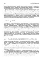
tables. Further, in pipes Manning’s n is a function of depth not a constant. Lanfear
and Coll (1978) state that at depths of 5 to 70 % of pipe diameter, n is 20 to 30 %

higher than the value for full pipe flow obtained from standard tables, failure to
account for this phenomena will cause flows to be overestimated by more than
20 %. For improved estimates of n, Wright (1991) recommended that Camp’s dis-
tribution of n as a function of depth (Figure 2.2.1) be used to adjust the value of
Manning’s n.
Wright (1991) presented the results of a field study for 22 sites in Grand Rapids
(MI, USA) that illustrates the accuracy of the typical application of Manning’s equa-
tion for estimation of flow in storm sewers. The pipes ranged in diameter from 45 to
243 cm, and in 5 of the 22 cases slopes were estimated fromfield measurements while
the remaining slopes were based on design drawings. The actual flow rate was esti-
mated using a hand-held electromagnetic velocity meter to measure the maximum
0
0.1
0.2
0.3
0.4
0.5
0.6
0.7
0.8
0.9
1
n/
/
n(full)
h/
/
D
1 1.1 1.2 1.3 1.4
Figure 2.2.1 Camp’s normalized distribution of Manning’s n versus relative depth in a circular

section
JWBK117-2.2 JWBK117-Quevauviller October 10, 2006 20:18 Char Count= 0
126 Sewer Flow Measurement
velocity and assuming that the mean velocity was 0.9 times the maximum velocity.
At the 22 sites discharge was measured an average of nine times, and the measured
discharge was used to calculate values of S
1/2
/n for each measurement. Average val-
ues of S
1/2
/n were determined for each site, and compared with the values of S
1/2
/n
for each site estimated from field conditions including the variation of Manning’s n
with flow depth (as would be done in the typical application of Manning’s equation).
The mean percent error was 28.9 %. In 50 % of the cases the errors were greater than
25 %, and in 27 % of the cases errors were greater than 50 %. Wright (1991) also
presented a case for sewers in Mobile, (AL, USA) that illustrated the even poorer
results obtained with Manning’s equation in pipes subject to surcharge and backwa-
ter. If a site is subject of surcharge and backwater, two stage gauges should be used,
and the water-surface slope should be used to approximate the energy slope. This
approach is rarely applied in practice.
Lanfear and Coll (1978) found that a ‘fitted’ Manning’s equation, calibrated by
a single flow measurement, provided good agreement with observed flow data and
eliminated the need to measure slope. A single discharge measurement is used to
calculate S
1/2
/n, which then is applied to all other flows. This approach was illus-
trated for multiple flow measurements in three 122-cm diameter brick sewers with
‘as built’ slopes between 0.00044 and 0.0144 in Washington (DC, USA). Lanfear

and Coll (1978) stated that if S
1/2
/n is determined for those flows of most concern,
most of the error caused by variable Manning’s n is eliminated. This implies that
if a wide range of flows are of interest, the value of S
1/2
/n may need to be cali-
brated throughout the flow range. Marsalek (1973) stated that under conditions of
unsteady, nonuniform flow in pipes, Manning’s equation underestimates flows in
the rising stage and overestimates flows in the falling stage. Finally, Alley (1977)
reported that the accuracy of the Manning’s equation technique is, at best, about
15 to 20 %.
2.2.3 FLUMES
Flumes have been used to measure open channel flows in small streams, irrigation
canals, water and wastewater treatment plants, and sewers for more than 50 years.
Flumes are flow-constriction structures that control the flow hydraulics such that
flow is directly related to head (Church et al., 1999). The most common type of
flume constricts the flow such that critical flow results somewhere in the constricted
section, which results in a unique relation between head and discharge as detailed
later. These flumes are known as critical-flow flumes. Flumes work best at sites
where the potential for surcharge, full-pipe pressurized flow, and backwater effects
are expected to be negligible. Flume measurements are reliable for both uniform and
nonuniform flow unless the sewer becomes surcharged (Parr et al., 1981). Baughen
and Eadon (1983) noted that flumes give misleading results if they are surcharged
and this condition is not suspected.
JWBK117-2.2 JWBK117-Quevauviller October 10, 2006 20:18 Char Count= 0
Flumes 127
The flow computation principle applied for critical-flow flumes may be derived
as follows (Wenzel, 1975). The energy conservation equation is applied between a
reference section 1 located immediately upstream of the flow constriction (flume)

and section 2 is located in the constriction a distance L downstream from section
(1) resulting in:
h
1
+ α
1
Q
2
2gA
2
1
+ z
1
= h
2
+ α
2
Q
2
2gA
2
2
+ z
2
+ h
L
(2.2.2)
where α is the kinetic energy correction factor, g is the acceleration of gravity, z is
the vertical distance from some datum, and h
L

is the head loss between sections 1
and 2. In the application of Equation (2.2.2) the following assumptions are made: (1)
steady flow; (2) hydrostatic pressure distribution at section 1; (3) small slope such
that the flow depth h approximately equals the vertical component of depth; and (4)
two- and three-dimensional effects are negligible or accounted for as coefficients or
energy loss terms (Wenzel, 1975). Equation (2.2.2) can be solved for discharge if all
other terms are measured or evaluated as follows:
Q =

2g(h
1
− h
2
+ LS
0
− h
L
)
α
2
A
2
2
−
α
1
A
2
1


1/2
(2.2.3)
where S
0
is the bed slope. If open channel flow is present and A
2
is sufficiently small,
critical flow will occur at some point in the constriction. If section 2 is defined as the
point of critical flow the following relation is derived from the fact that the Froude
number equals 1 for critical flow:
Q
2
B
2
gA
2
= 1 (2.2.4)
where B
2
is the width of the free surface at section 2. Substitution of Equation (2.2.4)
into Equation (2.2.3) and using known relations between A, h, and B, the discharge
can be implicitly determined by measuring only h
1
and evaluating h
L
, since all
other terms are known. The head loss can be determined from boundary layer theory
(Wenzel, 1975), but typically the relation between flow and discharge for a flume is
determined by laboratory ratings.
The Palmer–Bowlus flume was first proposed in the 1930s (Palmer and Bowlus,

1936), was extensively tested in the 1950s (Wells and Gotaas, 1958), and has be-
come the most commonly used critical-flow flume in sewer systems. Palmer–Bowlus
flumes have low head loss and can be installed in manholes where there is a stan-
dard, straight-through design, or they can be installed in the half section of the sewer
conduit (Soroko, 1973). Palmer–Bowlus flumes can be permanently installed, or be
portable devices which can be inserted in the downstream pipe of a manhole using
JWBK117-2.2 JWBK117-Quevauviller October 10, 2006 20:18 Char Count= 0
128 Sewer Flow Measurement
a pneumatic seal (Baughen and Eadon, 1983). Wells and Gotaas (1958) extensive
laboratory experiments on the Palmer–Bowlus flume indicated that accuracy within
3 % of the theoretical discharge is readily attainable at depths up to 0.9D (where D
is the upstream pipe diameter) for flumes installed in circular conduits. However,
Hunter et al. (1991) indicated that Palmer–Bowlus flumes typically are inaccurate
at depths greater than 0.75D.
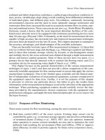
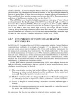
Figures 2.2.2 and 2.2.3 show two standardized trapezoidal Palmer–Bowlus flume
sections for which a rating table is presented in Ludwig and Parkhurst (1974). Ludwig
and Parkhurst (1974) noted that it is believed that the typical trapezoidal sections
offer advantages regarding flow range and the provision of more accurate mea-
surements at low flow values. Figure 2.2.4 shows a standardized rectangular throat
Palmer–Bowlus flume for which a rating table is presented in Ludwig and Parkhurst
(1974). Ludwig and Parkhurst (1974) noted that a value of D/10 represents a desir-
able rise in the base of rectangular flumes installed within circular conduits. Standard
Palmer–Bowlus flumes only have a stage measurement device in the approach sec-
tion. To measure pressurized full-pipe flow, pressure should be measured at both
sections 1 and 2 (approach and throat, respectively). Flumes with such two pressure
sensor designs are known as Venturi flumes, which are discussed in the following
paragraphs.
1
2
D/2

D/10
hc
hu
D
Figure 2.2.2 Standardized Palmer–Bowlus trapezoidal flume with a bottom width of one-half of
the pipe diameter
JWBK117-2.2 JWBK117-Quevauviller October 10, 2006 20:18 Char Count= 0
Flumes 129
1
2
D/3
D/10
hc
hu
D
Figure 2.2.3 Standardized Palmer–Bowlus trapezoidal flume with a bottom width of one-third
of the pipe diameter
hu
hc
D
B
T
t = D/10
Figure 2.2.4 Standardized Palmer–Bowlus rectangular flume
JWBK117-2.2 JWBK117-Quevauviller October 10, 2006 20:18 Char Count= 0
130 Sewer Flow Measurement
Venturi flumes act as critical-flow flumes during free-surface flows and as Venturi
meters during pressurized full-pipe flow. Equation (2.2.3) applies if the depth is
replaced by the pressure head, p/γ (where p is the pressure and γ is the specific
weight of the flowing fluid). For closed conduit flow Equation (2.2.3) becomes:

Q =

2g(H
1
− H
2
− h
L
)
α
2
A
2
2
−
α
1
A
2
1

1/2
(2.2.5)
where H is the piezometric head which equals p/γ + z. Assuming α
1
equals α
2
Equation (2.2.5) can be rewritten as follows forming the basic discharge equation
for a Venturi meter:
Q = C

D
⎡
⎢
⎣
2gA
2
2
H
1 −

A
2
A
1

2
⎤
⎥
⎦
1/2
(2.2.6)
where H = H
1
− H
2
, and C
D
is a discharge coefficient which accounts for head
loss and the nonuniform velocity distribution, α (Wenzel, 1975).
Diskin (1977) listed the following advantages of Venturi flumes:

(1) Ability to adapt the shape of the flume to the shape of the channel and the range
of flows expected.
(2) The possibility of predicting the coefficients of discharge either by theoretical
considerations or from the results of calibration tests.
(3) Relatively small head losses.
Venturi and critical-flow flumes also have the advantage of being self cleaning, i.e.
deposits may often be reduced to a minimum and the danger of clogging the down-
stream channel is small (Hager, 1989), and, thus, maintenance costs are minimal.
Diskin (1977) also noted that the disadvantage of Venturi flumes is the reduction in
channel width also lowers the pipe capacity, this is especially true in comparison to
the acoustic and electromagnetic flow meters discussed in the Sections 2.2.4–2.2.6.
Another disadvantage of Venturi flumes is that the relation between head and flow
breaks down in the transition zone from free-surface to pressurized flow. Such flows
are difficult to measure with any device because the flow pulsates from free-surface
to pressurized flow (Church et al., 1999).
The varying shapes that Venturi flumes can take is documented in the literature.
Kilpatrick and Kaehrle (1986) designed and calibrated a modified Palmer–Bowlus
(MPB) type flume for both open channel and pressurized full-pipe flow. The modi-
fication involved the use of a longer flume with flatter side slopes and a greater floor
thickness as well as adding a pressure sensor in the throat. The flume was designed
JWBK117-2.2 JWBK117-Quevauviller October 10, 2006 20:18 Char Count= 0
Flumes 131
so that its components could be passed through small manhole openings for assem-
bly in a trunkline sewer (i.e. D > 0.9 m). The MPB was tested in the laboratory
in 30.5- and 45.7-cm diameter pipes and in the field in a 122-cm diameter pipe.
The field tests involved controlled tests with hydrant flow and storm data. For the
hydrant flow, once each flow had stabilized, it was measured by both tracer dilu-
tion and acoustic meter; these discharges were in close agreement and also agreed
closely with the MPB flume calibration curves. The storm data consisted of 12 dye-
dilution measurements, which agreed well with the MPB and verified the laboratory

conditions.
Wenzel (1975) developed a Venturi flume in which the constriction consisted of
a cylindrical section with a radius greater than that of the pipe that could be fit-
ted with a symmetrical (two-sided) or an asymmetrical (one-side) configuration.
The theoretical rating developed from boundary layer theory was confirmed for
both open channel and pressurized full-pipe flow in laboratory experiments in a
20 cm diameter, 43 m long acrylic circular pipe. Diskin (1977) presented the re-
sults of laboratory evaluations of Venturi flumes with rectangular, trapezoidal, and
triangular throat shapes. B¨orzs¨onyi (1982) developed a Venturi flume involving a
lateral constriction of the channel. In free, open-channel flow and in pressurized
full-pipe flow the meter operates with accuracy better than ±5 %, and in submerged
open-channel flow the accuracy is estimated at ±8 %. Hunter et al. (1991) pro-
posed a Venturi flume with a truncated circular throat shape and transition slopes
of 1:6 for the entrance and exit sections of the constriction. Eight 25- and 30-cm
models were tested in two laboratories and it was found that this flume was ca-
pable of accurately measuring flows under conditions of free and submerged, for-
ward and reverse, free-surface flow, and forward and reverse pressurized full-pipe
flow.
Hager (1989) proposed and tested a substantially different critical-flow flume for
use in circular conduits. Rather than contracting the sides or bottom of the conduit to
cause critical flow, he proposed placing a cylinder in the centre of the pipe to cause
critical flow. Hager (1989) noted that the major advantages of this flume include
low cost, reading precision, insensitivity to submergence by backwater, and rapid
installation in running water. He also noted that the disadvantage of this flume is
that debris could get caught on the cylinder and clogging could result in sewers that
carry appreciable debris loads. Laboratory experiments with this flume found that
a diameter ratio of 0.3 between the pipe and the cylinder seemed optimal in terms
of approaching flow stability and discharge capacity, the tailwater depth may be at
least 80 % of the approaching flow depth (except for very low discharges), and the
maximum relative deviation of discharge from the flume rating curve was always

less than 3 %.
The accuracy of flow measurements is dependent on the accuracy of the construc-
tion and installation of the flumes in the pipe (i.e. level in a direction perpendicular
to flow, no deformation during construction or installation, no leakage at approach
section), and the measured geometry,slope, and friction of the flume surface (Church
et al., 1999). A well constructed, calibrated, and maintained flume may yield flows
JWBK117-2.2 JWBK117-Quevauviller October 10, 2006 20:18 Char Count= 0
132 Sewer Flow Measurement
with accuracies of 2–3 %, however, when factoring in the error of the stage measure-
ment device, the accuracy is about 5 % (Marsalek, 1973; Alley, 1977; Church et al.,
1999).
2.2.4 ELECTROMAGNETIC FLOW METERS
Electromagnetic flow measurement systems are based on Faraday’s law, which states
that the voltage induced ina conductor moving across amagnetic field is proportional
to the average velocity of that conductor (Doney, 1999a). If the cross-section were
rectangular with a uniform magnetic field, a true average velocity of the water in the
section would be obtained by measuring the induced voltage, but for nonrectangular
shapes and nonuniform magnetic fields the instrument must be calibrated (Newman,
1982). Electromagnetic flow measuring equipment measure pressurized pipe flows
with high accuracy (0.5 % according to Soroko (1973)) and has been available for
more than 30 years. Further, for full-pipe flows, Soroko (1973) reported that these
flow meters have no straight run requirements.
When electromagnetic flow meters were first applied to partially filled pipes re-
searchers were concerned that the presence of the free surface and the fact that
gravity flow is usually much slower than pressurized pipe flow would result in low
voltages that would be difficult to measure (Newman, 1982). However, Newman’s
(1982) practical experiments, supported by calibration tests at the British National
Engineering Laboratories, found that accuracies on the order of ±4 % could be
achieved for typical variations in flow profiles and backwater effects in a pipe.
Valentin (1981) also made an early application of an electromagnetic flow meter to

free-surface flow in a pipe and found that for depths between 0.5D and 0.8D errors
ranged from −4to−8 %and fordepths between 0.8D and D the error decreases from
−6to0%.
Doney (1999a) described a practical electromagnetic flow meter for use in par-
tially filled pipes. This instrument uses three pairs of electrodes located at different
flow heights in a flow tube to measure the induced voltage. The electronics unit of
the instrument selects the optimally located pair as a function of flow depth and
uses this pair to measure the induced voltage, which then is converted to the av-
erage velocity through a factory calibration. For full pipe flow the measurement
accuracy is 1 %, while for free-surface flow the accuracy is 3–5 % depending on fill
height. The instrument is accurate down to a flow depth of 10 %. The instrument
will measure sub- or supercritical flows and function with pipe slopes up to 5 %.
Finally, the meter requires straight runs of five pipe diameters upstream and three
downstream.
Soroko (1973) and Doney (1999a) list the following advantages of electromag-
netic flow meters: high accuracy, the ability to easily handle fluids with high solids
content, extremely wide range including reverse flows, obstructionless flow path,
minimal pressure loss, small straight pipe requirements, and low maintenance,
i.e. it is unaffected by grease on electrodes and silt and debris deposited in the
JWBK117-2.2 JWBK117-Quevauviller October 10, 2006 20:18 Char Count= 0
Area–velocity Flow Meters 133
invert (Baughen and Eadon, 1983). The primary disadvantages of electromagnetic
flow meters are high cost and difficult installation, especially in existing sewerage
systems.
2.2.5 AREA–VELOCITY FLOW METERS
Area–velocity flow meters (AVFMs) have become the most commonly used devices
for flow measurement in sewers. For example, the Milwaukee (WI, USA) Metropoli-
tan Sewerage District (MMSD) had 158 temporary and semipermanent flow mon-
itoring sites and 98 % of them had Doppler AVFMs (C. Schultz, MMSD, personal
communication, 2005). AVFMs have acoustic/ultrasonic or electromagnetic compo-

nents that are used to measure velocity at a point or throughout the profile (acoustic
only), which in turn is used to estimate the average velocity of the flowing fluid.
Depth also is measured and used to determine the flow area from the known sewer
geometry.The flowrate is the productof area and average velocity. MostAVFM man-
ufacturers report using these meters to measure submerged, surcharged, full-pipe,
and reverse flow conditions (the velocity range of most devices is −1.5 to 6.1 m/s).
The acoustic velocity measurement devices send continuous ultrasonic signals
and work as follows (Hughes et al., 1996):
When an ultrasonic beam is emitted into a fluid from an ultrasonic transducer, air
bubbles and dirt particles in the flow cause the ultrasonic beam to be scattered. This
scattering results in reflection of some acoustic energy in different directions, and the
reflected energy may be picked up by a receiving transducer, either at the same position
as the ultrasonic source or at some other position. If the fluid is in motion (relative to
the source) and the flow is stable, then the reflecting particles will have approximately the
same velocity as the moving fluid. The frequency of the reflected signal differs from the
frequency of the originally transmitted signal owing to the Doppler effect. The frequency
difference signal is known as the Doppler shift and is proportional to the velocity of the
particles in the fluid at the point of reflection.
The faster the object reflecting the sound waves moves in the water, the greater the
phase shift, or change in tone the meter registers (Day, 1996). In the typical Doppler
AVFM, a single ultrasonic beam directed on an angle into the flow from a single
transducer is used. The Sontek Argonaut SW uses two beams at an angle to the flow,
which increases the reliability and flow coverage of the instrument. Two types of
ultrasonic beam have been used:
(1) A narrow beam that measures the velocity in a small volume of the flow, typically
near the centre, an assumed velocity profile then is used to estimate the mean
flow velocity.
(2) A wide beam that attempts to measure the total velocity of the flow and determine
the average velocity directly.
JWBK117-2.2 JWBK117-Quevauviller October 10, 2006 20:18 Char Count= 0

134 Sewer Flow Measurement
The electromagnetic area–velocity meters operate similarly to the narrow-beam
Doppler AVFMs.
2.2.5.1 Narrow-Beam Doppler Area–Velocity Flow Meters
In a fairly clean pipe, with sufficient up and downstream straight runs, and an ax-
isymmetric velocity distribution, a fairly accurate average velocity will be rendered
with the narrow-beam Doppler AVFM (Day, 1996). However, it is very important
that an ideal or near-ideal velocity profile be present when utilizing a narrow-beam
Doppler or electromagnetic AVFM (Johnson, 1995; Day, 1996). The theoretical
velocity distribution used to compute the average velocity is based on uniform, tur-
bulent flow with no backwater effects (Hunter et al., 1991), and poor performance
can be expected when these conditions are not present. Inparticular, backwater due to
downstream flow restrictions is common in sewerage systems. Hughes et al. (1996)
had the following comments on the narrow-beam approach. This approach is suitable
for use in medium-sized sewers, but in larger sewers (>1 m diameter) the flow can
have steep velocity gradients with depth and large variations in velocity across the
section of the sewer flow. A single velocity reading derived from a volume near the
centre of the sewer flow is not always sufficient to produce a good representation of
the overall mean velocity of the flow. Previous studies using narrow-beam Doppler
AVFMs have suggested that in large sewers a single velocity reading may only be
accurate within ±20 %, even with sufficient depth (most meters need a flow depth
of at least 7.5 cm to make a velocity measurement, and higher depths are preferred)
and velocity of flow. However, under ideal conditions these systems can be accurate
within a few per cent. The performance of narrow-band Doppler AVFMs can be
improved through field calibration.
2.2.5.2 Wide-Beam Doppler Area–Velocity Flow Meters
Given the limitations of the narrow-beam Doppler AVFMs, most of the commer-
cially available AVFMs in common use apply the wide-beam approach (includ-
ing the ISCO, American Sigma and Automated Data Systems meters discussed in
Section 2.2.7); these are referred to as Doppler AVFMs from this point forward.

The primary concern for the wide-beam approach is whether the beam sufficiently
samples the total flow to get a true average. For example, if the flow distribution is
skewed and the ultrasonic beam is not of sufficient width, the true average may not
be obtained. Watt and Jeffries (1996) also found that the concentration and com-
position of particulates in the flow have a marked effect on the velocity measured
using Doppler AVFMs. They found that the fibrous waste from the paper making
process has an absorbent effect on the ultrasound signal resulting in modified read-
ings. They found similar results in the laboratory for sawdust. They reasoned that the
ultrasound signal fails to penetrate the highly polluted flow and the received signal is
JWBK117-2.2 JWBK117-Quevauviller October 10, 2006 20:18 Char Count= 0
Area–velocity Flow Meters 135
from a zone very close to the sensor.The main problem with trying to simultaneously
measure the entire flow at one time is ‘range bias’ wherein for deeper flows the dif-
ference in the strength of the return signal from particles close to the transducer and
those far away causes a distortion in the return signal frequency spectrum that is
difficult to resolve and typically results in the nearby, slower particles disproportion-
ally affecting the measurement, which then is biased low (Metcalf and Edelh¨auser,
1997).
2.2.5.3 Independent Evaluation of Doppler
Area–Velocity Flow Meters
Watt and Jefferies (1996) reported the results of extensive field and laboratory eval-
uation of Buhler-Montec Flow Survey Package Doppler AVFMs in the UK. This
involved laboratory and field checks of 6 monitors that had been deployed in the
field and evaluation of 59 monitors that had been used for short-term field studies.
The results of Watt and Jefferies (1996) are summarized in this section.
Field calibration of the depth sensors was carried out during each visit to the six
monitoring locations. Zero drift was found to be frequent, and in two of the six cases
it was greater than 5 cm, which was symptomatic of logger malfunction resulting in
the rejection of all data from these meters. The zero offset drifted low in five of the
cases, while three showed less than 0.5 cm drift in either direction. For all depths

greater than 10 cm the maximum error of any calibration prior to adjustment was
16 % with an average error of −2 %. When the absolute error was considered, this
latter figure became 3 % and when depths less than 25 cm were excluded the absolute
error dropped to 2 %. Field inspections of depth measurement showed substantial
need for calibration of the depth sensor.
Velocity measurements made by the six meters were evaluated in a 0.305 m
wide rectangular flume both before and after installation. In the flume for depths
greater than 10 cm the maximum velocity was 0.5 m/s. Although scatter was present
in the velocity readings, no evidence of zero error (bias) was found. A large part of
the scatter was attributed to turbulence in the flow resulting in fluctuations in the
response of the ultrasonic equipment. A linear regression fit to the data indicated
that, on average, the AVFM velocity was 5.6 % lower than the true mean velocity.
The average absolute error ranged from 12 to 26 % at velocities less than 0.3 m/s
and reduced rapidly at higher velocities. The data suggested that average errors
no greater than 5 % in velocity should be expected at mean velocities greater than
0.5 m/s.
The final evaluation of Doppler AVFM usefulness involved a short-term flow
survey in which 59 monitors were used for model verification. Five of the 59 monitors
were found, after comparison with the model, to have yielded data that were so poor
that they could not be used. In general, the flows were unbelievably high and three of
the five were detected during comparisons with data from nearby sites at which flow
discrepancies of up to 200 l/s were found. No specific reasons for the poor quality of
JWBK117-2.2 JWBK117-Quevauviller October 10, 2006 20:18 Char Count= 0
136 Sewer Flow Measurement
data at these sites could be found, and the quality assurance checks were insufficient
to prevent such data errors. Watt and Jefferies (1996) considered it disturbing that
the data were rejected at the model verification stage and the fact that the majority
of monitors giving poor data were found in this way raised questions as to validity
of the data from other sites where no checking was possible. The accuracy of the
verified model was, as a consequence, questioned in spite of a reasonable number

of calibration readings taken.
At all sites, 35 % of the peak stage values during the verification events were
greater than three times the highest calibration value and the corresponding value
for velocity was 25 %. Thus, the field calibration of the Doppler AVFMs relied on
recorded data from a small portion of the range of measurements to be made by the
instruments. This may have contributed to the poor results at the five sites, but it
does not explain why only these sites.
Watt and Jefferies (1996) quoted the UK Water Research Centre guide to short-
term flow surveys in sewer systems as stating the following:
An accuracy in the region of ±10 % can be obtained with the measurement of flow when
using a velocity and depth monitor provided that:
(i) The instrument is fully serviceable and working in accordance with the specifica-
tion.
(ii) The site has suitable hydraulic characteristics.
(iii) There is adequate flow for accurate measurement by the instrument.
If an approximate velocity calibration has to be applied, the accuracy of the results will
be reduced and an accuracy of ±10 % cannot be expected.
Watt and Jefferies (1996) noted that in practice, the accuracy of the flows calculated
will frequently be poorer than ±10 %, even though the UK Water Research Centre
requirements are met. Nonetheless, Watt and Jefferies (1996) concluded that flow
rates in small sewers without extreme velocities were found to be accurate within
±7%.
2.2.5.4 Summary
AVFMs have many practical advantages including ease of installation, portability,
and reasonable cost. Also, Day (1996) noted that the electronic packages for all of
the Doppler AVFMs on the market adapt well to the sewer environment (moisture,
corrosion, etc.), and that a unique feature of Doppler AVFMs that has been observed
in the field is the ability to fire under mild fouling conditions and maintain reason-
able accuracy. Doney (1999b) stated that manufacturers typically report accuracy as
±2 %. However, the literature search conducted here indicated that accuracies be-

tween 10 % and 30 % may be more likely without on-site calibration, and even after
calibration a large range in accuracy for given events may result. Further, useful field
JWBK117-2.2 JWBK117-Quevauviller October 10, 2006 20:18 Char Count= 0
Acoustic Doppler Profiler Flow Meters 137
calibration is difficult to achieve because the majority of checks are carried out for
dry weather flows, while much of the interest in the results may be for storm flows
(Watt and Jefferies, 1996). The accuracy of Doppler AVFMs relies on: the inherent
accuracy of the equipment; its maintenance prior to installation; the quality of field
site checks; site conditions; and a range of operational factors (Watt and Jefferies,
1996). Finally, Day (1996) noted that the performance of Doppler AVFMs is un-
certain in large pipes (i.e. over 150 cm) simply from a lack of testing, however, for
pipes under 91 cm, Doppler AVFMs have proven to be accurate (given the previously
stated caveats) and repeatable.
2.2.6 ACOUSTIC DOPPLER PROFILER FLOW METERS
The acoustic Doppler profiler flow meter (ADFM) was exclusively developed
by MGD Technologies Inc. (Complete details on the ADFM may be found at:
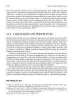
The ADFM uses the Doppler shift principle to deter-
mine the velocity of flowing water, but instead of using a continuous ultrasonic
signal as done with Doppler AVFMs, the ADFM emits short ultrasonic pulses called
‘pings’ into the water from each of four transducers that are angled into the flow
(Figure 2.2.5). The ADFM range-gates the return signal from each ping allowing
the ADFM to measure the velocity in many small volumes (called bins, cylinders
about 4 cm in diameter and 5 cm long) that are regularly spaced throughout the
water column. The velocity in each volume is measured independently, so that an
independent velocity profile is obtained for each beam (Metcalf and Edelh¨auser,
1997). There can be as many as 40 discrete bins in a 2 m deep flow. Narrow beams
are used to minimize errors related to beam width. Since the acoustic pulses are very
short and the velocity is measured in small bins, range bias is virtually eliminated
VELOCITY PROFILE #2
VELOCITY PROFILE #1

DEPTH CELLS
FLOW PATTERN
TRANSDUCER
Figure 2.2.5 Schematic representation of the acoustic Doppler profiler flow meter (ADFM)
measurement operation. (Provided by M. Metcalfe, MGD Technologies Inc.)
JWBK117-2.2 JWBK117-Quevauviller October 10, 2006 20:18 Char Count= 0
138 Sewer Flow Measurement
(Metcalf and Edelh¨auser, 1997). Thus, the ADFM obtains an accurate measurement
of the velocity distribution within a pipe or channel both vertically and transversely.
The velocity data from the profiles are entered into an algorithm to determine
a mathematical description of the flow velocities throughout the entire flow cross-
section. The algorithm fits a parametric model to the actual data. The result predicts
flow velocity at every point throughout the flow, the velocity distribution then is inte-
grated over the cross-sectional area to determine the discharge (Curling et al., 2003).
As hydraulic conditions change, the change will manifest itself in the distribution of
velocity throughout the vertical. Thus, the ADFM does not require at site calibration.
Each time the ADFM pings, it collects velocity data. These data have a random
error associated with them, which can be reduced by averaging many pings together
into an ensemble. From sampling theory, the ensemble standard deviation is equal
to the standard deviation of a velocity measurement for a single ping divided by
the square root of the number of pings in an ensemble. Typically, the averaging
of 400 pings takes only a few minutes (Metcalf and Edelh¨auser, 1997). Thus, it is
possible to get extremely precise estimates of velocity at a fairly rapid rate, avoiding
the high degree of noise in the velocity data common for Doppler AVFMs (see
Section 2.2.7).
The MGD Internet site ( provides the results of seven
extensive laboratory and field tests of the ADFM. In each case the ADFM was placed
in the centre of the channel or pipe and measured the flow without site calibration.
The seven tests were as follows:
(1) Testing in rectangular flumes 1.22 and 3.66 m wide in the US Bureau of Recla-

mation Water Resources Research Laboratory.
(2) Field checking by Brown and Caldwell Inc. of measured flow in a 183 cm
diameter concrete combined sewer interceptor in Onondaga County (NY, USA)
using dye dilution.
(3) Field checking by Brown and Caldwell Inc. of measured flow in a 274 cm
diameter concrete sewer line in Sacramento (CA, USA) using dye dilution.
(4) Laboratory testing in a 38 cm diameter PVC pipe done for the Pima County
(AZ, USA) Wastewater Management Department.
(5) Field testing in the Salt River Project (AZ, USA) Arizona Canal in comparison
with a rated broad-crested weir.
(6) Testing in a 76.2 cm diameter concrete test pipe in the US Department of
Agriculture Water Conservation Laboratory.
(7) Testing in a 122 cm diameter concrete pipe and 0.91 and 2.13 m wide rectangular
flumes at the Utah Water Research Laboratory of Utah State University.
Metcalf and Edelh¨auser (Metcalf and Edelh¨auser, 1997) also reported the results of
tests in a 0.6 m wide rectangular flume at the Australian Water Technologies office in