Integrated Waste Management – Volume I

516
4.3 Human resources performance indicators
Human resources indicators determined, reveal that the 22 LPT where information was
reported, 60% only have one operator, 31% two operators, and 9% three operators. It should
be noticed that the number of operators reported by the ME in general do not account for
the superior technician responsible for the LTP management. It is also noticed that in the
case of small LTP operators are not entirely affected to LTP operation.
Concerning specific learning on LTP operation, only five cases referred conducting annually
learning actions on LTP, mainly where reverse osmosis processes are used and in the case of
the evaporation condensation treatment system.
4.4 Operational performance indicators
About problems identified on LTP functioning, ME reported in general operational and
logistics problems and in a lesser extent personnel and other problems (Table 2). The
operational problems identified were in general equipment damages, leachate storage
capacity limitations, raw leachate quality treatability, as well as, in the case of reverse
osmosis membrane reactors, high maintenance needs. Of the 23 ME that reported these
problems, 40% indicated a monthly frequency and 32% a weekly frequency. In terms of
logistic problems, eight ME reported mainly reagents supplies problems, three of them with
a monthly frequency, other three rarely (i.e. once a year) and one with a daily frequency.
Four ME, one with an annual frequency and three on a weekly basis reported personnel
problems. The mentioned problems refer to lack of specialized personnel for the treatment
system’s operation. Five ME also mentioned other problems with a monthly frequency,
however not specifically defined.

Problems Operational Logistics Personnel Other
Type
Equipment damages
Reagents supplies

Lack of
specialized
personnel
Not specified
Leachate storage
capacity limitations
Reverse osmosis
membrane reactors,
high maintenance
needs
Raw leachate quality
treatability
Frequency
of
occurrence
23 reported:
-13% weekly
-32% monthly
-40% per trimester
-13% yearly
8 reported:
-1 weekly
-1 monthly
-3 per trimester
-3 yearly
4 reported:
-1 weekly
-3 yearly



5 reported:
-5 weekly



Table 2. Problem types and frequency of occurrence at reported LTP
Regarding leachate and groundwater monitoring and according to the information given by
the ME in the questionnaires of 27 landfills, in 21 (78%) 100% of the number of leachate
parameter analysis defined in the legislation or in the landfill environmental license were
done. Five landfills performed between 80% and 99% of the total number of analysis. As for
groundwater monitoring where information was given, 54% (i.e. 13 of 24 landfills)

Performance Indicators for Leachate Management: Municipal Solid Waste Landfills in Portugal

517
performed all parameter analyses legally defined, seven landfills between 80% and 99%, and
the remaining four landfills below 79% of the number of groundwater parameter analysis.
LTP energy consumption was also determined and an annual average of 11.1 kWh/m
3
of
leachate was obtained, with values varying between 1.8 kWh/m
3
and 38.0 kWh/m
3
.
4.5 Financial and economic performance indicators
Concerning LTP cost analysis, the performance indicators attempted to translate LTP overall
costs. Results are based on the information reported in the questionnaires, however ME only
reported this information for 17 LTP, lacking information on few cost components in some
cases. On the other hand, the values obtained are relevant for reference and comparison

between the LTP treatment systems.
Average overall unit costs (i.e. per unit of raw leachate treated in LTP) for the year 2006 was
8.8 €/m
3
, 6.1 €/m
3
referring to current expenses costs and 2.7 €/m
3
to capital costs (i.e.
capital amortizations in 2006). In terms of main treatment systems, treatments that use
macrophyte beds revealed to be the less expensive (2.4 €/m
3
). The evaporation
/condensation process, recently being used in one LTP, presented the highest capital costs
(25.0 €/m
3
). The ME did not report in this case current expenses costs and total unit costs
could not be determined. Other treatments refer to all remaining treatments systems
presented in Table 1. Except for the evaporation/condensation treatment system, the
average unit cost for these treatments is the higher obtained (8.5 €/m
3
), mainly due to one of
the LTP that presented higher costs comparing with other LTP with similar treatment
systems (i.e. in terms of treatment system reconstruction costs and current expenses costs),
thus increasing the unit cost. Comparing with other treatments systems the reverse osmosis
membrane process presented on average higher capital costs (3.3 €/m
3
).
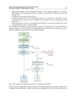
Percentage distribution of current expenses costs obtained (Figure 6) revealed that on
average 67% refer to other current expenses costs (e.g. reagents, equipment rental, service

acquisitions and other costs), 23% refer to energy costs for LTP operation, and the remaining
10% to personnel costs.
4.6 Service quality performance indicators
The main leachate contaminants (BOD
5
, COD, total nitrogen and TSS) removal efficiencies
were determined for 21 LTP. Taking in account the information on raw leachate and treated
leachate quality monthly information for 2006, reported in the questionnaires by the ME,
Table 3 presents removal efficiencies obtained for the main treatment systems.
As previously presented, treatment systems with macrophyte beds are less expensive,
although the removal efficiencies are rather low (Table 3). In the case of total suspended
solids, no removal was obtained. Considering the discharge to sanitary sewers this
treatment option can be economic. The reverse osmosis membrane process revealed to be
the most contaminant removal efficient treatment option as it is mainly used when
discharge to streams is the only option. Although only COD removal efficiency was possible
to determine for the evaporation/condensation process, it also shows to be a possible
option, however expensive, for full treatment on-site and discharge to streams. The
remaining treatments systems of nine LTP showed various removal efficiencies for the
considered parameters. These treatment processes are mainly used for partial treatment on-
site, and further complete treatment at PWTP. With respect to pH, all LTP effluents
complied with legal limit values (i.e. pH between 6 and 9) for discharge to stream.

Integrated Waste Management – Volume I

518

Fig. 6. Percentage distribution of current expenses costs for reported MSW landfills

Main leachate treatments
Number

of LTP
Removal efficiency (%)
COD Total Nitrogen TSS
Min Max Average Min Max Average Min Max Average
Macrophyte beds 2 26.6 49.3 37.9 17.4 17.4 17.4 No removal
Reverse osmosis 9 98.6 99.9 99.6 99.3 99.8 99.6 87.9 99.5 93.7
Evaporation/Condensation 1 99,9 Not available Not available
Other treatments 9 53.0 89.6 69.0 29.0 46.6 37.8 18.8 94.9 54.2

Table 3. Average, minimum, and maximum leachate contaminant removal efficiencies for
the main treatment systems
4.7 Opinion indicators
This group of indicators pretended to transmit the questionnaires’ respondent, in general
LTP or landfill managers, about LTP performance. Results are presented in Figure 7. In the
case of adequacy of the treatment system to leachate quantity, 48% of the respondents
positioned in the middle (i.e. nor satisfied, nor unsatisfied). Similar percentage of responses

Performance Indicators for Leachate Management: Municipal Solid Waste Landfills in Portugal

519
(26%) was obtained both for the positive pole (i.e. satisfied or very satisfied) and for the
negative pole (i.e. unsatisfied or very unsatisfied). In terms of leachate quality, 60% of the
responses were in the middle position, although 29% were negative, revealing that
managers are more concerned about leachate quantity than quantity on the adequacy of the
leachate treatment systems.


Fig. 7. Opinion indicators results
5. Conclusion
Performance indicators and relevant context information can be a valuable tool on MSW

landfills leachate management assessment and benchmarking analysis. With the application
of the proposed performance indicators to the leachate treatment and management in
Portugal’s mainland it was possible to identify the most cost and contaminant removal
efficient treatments systems, among several constrains regarding the lack of specific
definitions on leachate discharge quality limits to streams and lakes, considering the
particular characteristics of this effluent. To discharge in sanitary systems, more economic
treatments can be used, however legal definition and uniformity regarding discharge
quality limits in domestic wastewater collection systems is also needed. In the case of old
dumps, the monitoring and management is generally defined on national legislation.
Therefore, a need for management definition and for leachate monitoring parameters
generated by closed dumps would be an improvement in this matter.
On the other hand, most problems identified possibly relate to an inadaptability of general
leachate production and quality models with the national specific meteorological and
landfill operation conditions. On this matter, an historical assessment on MSW landfills
could be developed to adapt existing models to the Portuguese context. Regarding leachate
and concentrate recirculation on current operational MSW landfills, further studies to assess

Integrated Waste Management – Volume I

520
economic and environmental costs and benefits should also be developed. In this way, legal
authorities could have relevant information for decision making in modifying existing
legislation on this matter.
6. Acknowledgment
Considering the relevancy of this study in the scope of his mission as the sector regulatory
entity, the present study was financed by the Portuguese Waste and Water Regulatory
Institute (IRAR).
The Authors also wish to thank all MSW management entities that participated in this study
and technicians that contributed to the questionnaire survey.
7. References

Alegre, H.; Hirner, W.; Baptista, J. M. and Parena, R. (2004). Indicadores de desempenho para
serviços de águas de abastecimento – Série Guias Técnicos 1, Estudo realizado pelo
LNEC para o IRAR, Portugal
Bicudo, J. R. and Pinheiro, I. (1994). Caracterização quantitativa e qualitativa das águas lixiviantes
do aterro intermunicipal de Loures e Vila Franca de Xira, Relatório 156/94 – NES,
LNEC, Portugal
Ehrig, H. J. (1983). Quality and quantity of sanitary landfill leachate. Waste Management
Research, Vol.1, No.1, (January 1983), pp. 53-68, ISSN: 1096-3669
IRAR and APA (2008). PERSU II: Plano Estratégico para os Resíduos Sólidos Urbanos 2007-2016.
Relatório de Acompanhamento 2007, Instituto Regulador de Águas e Resíduos (IRAR)
and Agência Portuguesa do Ambiente (APA), Portugal
Levy, J. and Santana, C. (2004). Funcionamento das estações de tratamento de águas lixiviantes e
acções para a sua beneficiação, INR /CESUR, Portugal
Matos, R.; Cardoso, A.; Ashley, R.; Duarte, P.; Molinari, A. and Shulz, A. (2004). Indicadores
de desempenho para serviços de águas residuais – Série Guias Técnicos 2, Estudo
realizado pelo LNEC para o IRAR, Portugal
Martinho, M.G.; Santana, F.; Santos, J.; Brandão, A. and Santos, I. (2008). Gestão de Lixiviados
de aterros de RSU. Relatório Técnico n.º 3/2008, Faculdade de Ciências e Tecnologia
and Instituto Regulador de Águas e Resíduos edition, December 2008, ISBN 978-
989-95392-5-9
Martinho, M.G.; Santos, J.; Brandão, A. and Nunes, M. (2009). Leachate management at
municipal solid waste landfills in Portugal, Proceedings of the Twelfth International
Waste Management and Landfill Symposium, Sardinia, Italy, October 5-9, 2009
MAOTDR (2007). Plano Estratégico para os Resíduos Sólidos Urbanos 2007-2016 (PERSU II).
Ministério do Ambiente, do Ordenamento do Território e do Desenvolvimento
Regional, Séries de Publicações MAOTDR, Portugal
McDougall, F. R.; White, P. R.; Frankie, M. and Hindle, P. (2001). Integrated Solid Waste
Management: a Life Cycle Inventory. 2nd Edition, Blackwell Publishing, Oxford.Lima,
P.; Bonarini, A. & Mataric, M. (2004). Application of Machine Learning, InTech, ISBN
978-953-7619-34-3, Vienna, Austria

Qasim, S.R. and Chiang, W. (1994) Sanitary landfill leachate – generation control and treatment.
Technomic Publishing Company, Inc. Lancaster, USA
27
Measurements of Carbonaceous
Aerosols Using Semi-Continuous
Thermal-Optical Method
Yu, Xiao-Ying
Pacific Northwest National Laboratory
USA
1. Introduction
Waste management involves collection, transport, processing, recycling, disposal, and
monitoring of waste materials that can be solid, liquid, gaseous, or radioactive, which all are
generated by human. It is important to monitor aerosols emitted during waste treatment
and management to understand their impact on human health and the environment.
Carbonaceous aerosols are major components in air pollution as a result of energy
consumption, thus measurement of them is important to waste management. Increasing
interest has been drawn to the identification, measurement, analysis, and modeling of
carbon aerosols in the past decade. This book chapter will provide a review of the widely
used semi-continuous thermal-optical method to determine carbonaceous aerosols in
relation to air pollution and waste management.
Quantification of carbonaceous species provides important observations in understanding
aerosol life cycle. Carbonaceous aerosols play important roles in air quality, human health,
and global climate change. However, accurate measurement of carbonaceous particles still
presents challenges. Carbonaceous particles are divided into three categories: organic
carbon (OC), elemental carbon (EC), and inorganic carbonate carbon (CC) [Chow et al., 2005;
Schauer et al., 2003]. The terms “elemental carbon (EC)“, “soot”, “black carbon”, “graphic
carbon”, and “light absorbing carbon” are often used loosely and interchangeably in
different research areas. Atmospheric EC particles are produced almost exclusively under
incomplete combustion conditions. They are from both anthropogenic and biogenic
emissions. Ambient elemental carbon particles rarely appear as diamond crystalline

structure. EC aerosols absorb light effectively and they can be characterized by light
scattering, absorption, or transmittance, as well as other methods. Absorption spectroscopy
is deemed to provide quantitative information of EC. Difference in the definition of EC is a
result of measurement methods [Jeong et al., 2004; Watson et al., 2008].
Increasingly OC has drawn more attention because of its effect on regional air pollution and
global climate change. OC aerosol formation is attributed to both biogenic and
anthropogenic sources [Bond & Bergstrom, 2006]. OC may be released directly into the
atmosphere (primary organic aerosol) or formed when gaseous volatile organic compounds
are released to the atmosphere followed by photolysis induced oxidation to form secondary
organic aerosols [Bae et al., 2004; Schauer et al., 2003]. Past findings indicate that a large

Integrated Waste Management – Volume I

522
percentage of OC observed around the world is secondary [Zhang et al., 2007]. This chapter,
however, focuses on the widely used semi-continuous thermal analysis method.
Comparisons among relevant methods are also provided.
2. Thermal desorption analysis methods
Thermal desorption has been used to analyze volatile organic compounds. The physical
principle lies in the fact that different components of a sample volatize, oxidize, or react
with other reagents as the temperature profile changes [MacKenzle, 1970]. Many methods
employ a two-step temperature profile. Generally speaking, sample is heated in the first step
to a temperature ranging from 350 C to 850 C. Carbon evolved in this step is defined as
OC. In the second step, sample is heated to a temperature ranging from 650 C to 1100 C.
Carbon evolved in this step is defined as EC. At the first temperature regime, the
volatilization rate of EC is assumed to be low, and OC evolution occurs in an atmosphere
without an oxidizing agent. Carbon dioxide (CO
2
) gas forms as a result of OC evolving from
the sample. In step 2, an oxidizer is introduced. Oxygen (O

2
) is often used. EC reacts with
this oxidizing agent, sometimes under catalysis conditions, to form CO
2
. CO
2
is detected
directly. A methane (CH
4
) – helium (He) mixture is used to calibrate the system; the CH
4
is
oxidized in the same manner to achieve quantification. The original compounds are
transformed due to thermally-induced reactions (dissociation or oxidation). The detection is
not chemically specific using the thermal analysis method. Results are often reported as
empirically and operationally defined categories including OC, EC, and TC. TC is the sum
of OC and EC (TC=OC+EC).
An important factor in thermal evolution methods is the OC/EC split point. Many methods
use Optical Reflectance and/or Optical Transmission to monitor the conversion of OC to EC
and the oxidation of EC to CO
2
. The rationale is that since EC is not volatile until very high
temperatures (well above the ~840 C used by the NIOSH method, for example), its release
is only dependent on oxidation when oxygen is present. High temperatures in the non-
oxidizing environment often cause some OC components to form EC by charring. This
complicates the determination of EC as additional EC is formed due to this charring. When
oxygen is added to the sample oven, the black EC char will combust and the filter becomes
white. When the light intensity from reflection or transmission of the samples on the filter
reaches its original intensity, the charred OC is assumed to be removed. The OC/EC split
point is usually defined in this manner. It is assumed what comes off after the split point is

quantitatively nearly equal to the EC that was on the filter originally as EC.
Thermal-Optical methods assume that: (1) The EC caused by charring of OC’s during the
first O
2
-free step is more easily oxidized; or (2) that the absorption coefficient of the EC
formed by charring is similar to the absorption coefficient of the original EC within the filter.
If either of these assumptions is correct, then the method will be an effective quantitative
method of OC and EC. Although the operational principle is similar, subtle differences exist
among the different methods. These factors may include analysis atmosphere, temperature
profiles, optical monitoring approaches, sample size, and other differences in physical
configurations of the analytical instrument [Watson et al., 2005; Chow et al., 2005]. Some
examples of more detailed studies of the effect of using TOT and TOR on the OCEC split
point are discussed elsewhere [Chow et al., 2004; Cheng et al., 2009].
Particulate samples are usually collected using filters ranging from several hrs to days, then
samples are prepared for off-line analysis in the laboratory. For OC and EC laboratory

Measurements of Carbonaceous Aerosols Using Semi-Continuous Thermal-Optical Method

523
analysis, the Sunset instrument (Sunset Laboratories Inc.) and the DRI (Desert Research
Institute) instrument are among the most commonly used. Near real-time or real-time on-
line techniques are advantageous compared with off-line ones, because they provide faster
sampling resolution and reduce labor in analysis. More importantly, the faster time
resolution makes it possible to capture fast changing fluctuations of particle emisisons,
where the off-line methods would have missed due to the longer sampling time.


Fig. 1. An example of the modified NIOSH thermo-optical analysis thermal desorption
diagram of a field sample. The x-axis is time in seconds, and y-axis is intensity of different
traces. The blue color is oven temperature; red NDIR laser intensity; gray pressure; and

green carbon dioxide.
Several techniques are established for in situ determination of black carbon (BC), such as the
aethalometer and the particle soot absorption photometer. The relationship between BC and
EC, however, is not fully resolved. These on-line EC methods do not provide OC
measurements simultaneously. The Sunset Semi-Continuous Organic Carbon/Elemental
Carbon (OCEC) Aerosol Analyzer has been a successful development for on-line OC and EC
measurement. It can provide measurements of OC and EC on hourly time scales,

and it
allows for semi-continuous sampling with analysis immediately after sample collection. The
instrument provides quantification of both OC and EC aerosols and requires no off-line
sample treatment and laboratory analysis. This reduction in complexity, along with the
ability to measure OC and EC on an hourly basis, provides advantages over conventional
off-line integrated techniques.
Aerosol light absorption can be used to determine EC (or BC) either on filter media or in
situ. There are several commerically avaialble instruments based on aerosol light absorption
including the aethalometer, particle soot absorption photometer (PSAP), micro soot sensor,
multi-angle absorption photometer (MAAP), photo-acoustic soot spectrometer (PASS), and
single particle soot photometer (SP2). Moosmüller et al. [2009] provides a detailed review of
these techniques. Due to the commericial avaiability of these fast in situ instruments, more
comparisons have been made to the EC measurements among them. Instrument uncertainty
and minimum detection limits were determined for these techniques. Some recent examples
of these quantities and comparisons are seen in Chow et al. [2009], Cross et al. [2010],
Slowick et al. [2007].
Other newer developments often involve mass spectrometery. One such successful example
is the aerosol mass spectrometer [Jayne et al., 2000]. However, it does not provide

Integrated Waste Management – Volume I

524

simultaneous EC measurements, although it can provide faster resolution of total organic
aerosol. The latter is often deduced to primary and secondary components using positive
matrix factorization (PMF) analysis. As a result, it is more labor intensive to operate and
conduct data reduction. In addition, MS based instruments are often more expensive to
purchase. They take more power and space, therefore, not immediately accessible for long-
term regulatory monitoring purpose in waste management.
2.1 The Sunset OCEC analyzer
The semi-continuous Sunset OCEC analyzers (Model 3F, Sunset Laboratory Inc., Portland,
OR) is widely used to measure OC and EC mass loadings at different locations. Ambient
samples were collected continuously by drawing a sample flow of ~8 lpm. A cyclone was
used upstream of the instruments to pass particles smaller than 2.5 µm. The airstream also
passed through a denuder to remove any volatile organic compounds in the air. Sample
flow rate was adjusted for the pressure difference between sea level and each of the sites to
ensure accurate conversion of sample volume. During automated semi-continuous
sampling, particulate matter was deposited on a quartz filter. The quartz filter was normally
installed with a second backup filter, mostly to serve as support for the front filter. The
portion of the sample tube containing the quartz filter was positioned within the central part
of an oven, whose temperature was controlled by an instrument control and data logging
program installed on a laptop computer and interfaced with the OCEC instrument.
After a sample was collected, in situ analysis was conducted by using the modified NIOSH
method 5040, i.e., thermal optical transmittance analysis, to quantify OC and EC. The oven
was first purged with helium after a sample was collected. The temperature inside the oven
was ramped up in a step fashion to ~ 870 °C to thermally desorb the organic compounds.
The pyrolysis products were converted to carbon dioxide (CO
2
) by a redox reaction with
manganese dioxide. The CO
2
was quantified using a self-contained non-dispersive infrared
(NDIR) laser detection system. In order to quantify EC using the thermal method, a second

temperature ramp was applied while purging the oven with a mixture containing oxygen
and helium. During this stage, the elemental carbon was oxidized and the resulting CO
2
was
detected by the NDIR detection system. At the end of each analysis, a fixed volume of
external standard containing methane (CH
4
) was injected and thus a known carbon mass
could be derived. The external calibration was used in each analysis to insure repeatable
quantification. The modified NIOSH thermal-optical transmittance protocol used during a
field study in Mexico City is summarized in Table 1.
Errors induced by pyrolysis of OC are corrected by continuously monitoring the absorbance
of a tunable diode laser beam (λ = 660 nm) passing through the sample filter. When the laser
absorbance reaches the background level before the initial temperature ramping, the split
point between OC and EC can be determined. OC and EC determined in this manner are
defined as Thermal OC and Thermal EC. Total carbon (TC) is the sum of Thermal OC and
Thermal EC, TC = Thermal OC + Thermal EC, or TC=OC+EC. The Sunset OCEC analyzer
also provides an optical measurement of EC by laser transmission, i.e. Optical EC. Optical
OC can be derived by subtracting Optical EC from total carbon, Optical OC = TC - Optical
EC, where TC is determined in the thermal analysis.
Modifications can be made to the temperature steps in the thermal-optical method. Conny et
al. [2003] conducted a study to optimize the thermal-optical method for measuring
atmospheric black carbon employing surface response modeling of EC/TC, maximum laser
attenuation in He, and laser attenuation at the end of the He phase. They tried to minimize

Measurements of Carbonaceous Aerosols Using Semi-Continuous Thermal-Optical Method

525
the positive bias from the detection of residual OC on the filter as native EC by maximizing
the production OC char by the Sunset (TOT) instrument. In addition, they sought to

minimize the negative bias from the loss of native EC at high temperatures. This first study
concluded that for particle samples around 30 to 50 µg, the optimal condition for steps 1- 4
in the He environment are 190 ºC for 60 s, 365 ºC for 60 s, 610 C for 60 s, and 835 C for 72 s,
respectively.

Carrier Gas Duration (sec) Temperature (ºC)
He-1 10 Ambient
He-2 80 600
He-3 90 870
He-4 25 No Heat
O
2
-1 30 600
O
2
-2 30 700
O
2
-3 35 760
O
2
-4 105 870
CalGas 110 No Heat
Table 1. An example of the modified NIOSH 5040 thermal-optical protocol used during the
MILAGRO campaign [Yu et al., 2009].
Recently, Conny et al. [2009] reported an update using the same empirical factorial-based
response-surface modeling approach to optimize the thermal-optical transmission analysis
of atmospheric black carbon. They showed that the temperature protocol in the TOT
analysis of a Sunset Instrument can be modified to distinguish pyrolyzed OC from BC based
on the Beer-Lambert Law. The optimal TOT step-4 condition in the helium environment was

established to be around 830 - 850 C using urban samples via response surface modeling in
their newer findings, although temperature as low as 750 C or as high as 890 C is not
excluded. This optimization is based on two criteria. First, sufficient pyrolysis of OC must
occur in the high temperature helium environment (i.e., He step 4 or the high temperature
step in He), so that insufficiently pyrolyzed OC is not measured as native BC after the split
point. Second, the apparent specific absorption cross sections of OC char and the apparent
specific absorption cross sections of native BC determined by the instrument are assumed to
be equivalent to determine the optimal operation conditions.
2.2 Aerosol sampling inlet and field deployment
In order to eliminate interference from near ground activities, an aerosol sampling stack can
be used adjacent to the dwelling hosting the instrument at a surface site. An example is
given below based on our field deployment experience. The sampling stack is made of PVC
pipe ~ 20 cm in diameter and extending ~ 8 m above ground. The stack inlet is protected by
a rain cap. A heated stainless steel sampling intake tube (~ 5 cm in diameter) is coaxially
positioned in the center of stack ~ 4 m below the top of the stack and extending through the
lower end cap. The airflow through the aerosol sampling stack is ~ 1000 lpm, of which
approximately 120 lpm is drawn into the heated tube. The tube is wrapped with heating
tape and insulation and further encased in a PVC pipe. Electric power is applied to heat the

Integrated Waste Management – Volume I

526
sample line such that the relative humidity (RH) of the sample air is maintained at or below
40%. Much simpler design can be used to obtain equally good sampling results.
Filters are recommended to be changed every few days before the laser correction factor
reached below ~ 90%. Sampling interval shall be determined based upon local mass
loadings. At locations with low mass loadings that are close to the instrument detection
limits, it makes sense to sample for longer time. Otherwise, for semi-real time sampling, the
sample time is usually chosen to be one hour, i.e., 45-minute ambient sampling followed by
15 minutes thermal-optical analysis. Daily, at midnight, a 0-min sampling blank is taken.

Instruments should be calibrated using an external filter with known OC and EC mass
concentrations. Values reported are corrected to ambient temperature and pressure, this is
especially important if the sampling location is elevated. Externally produced standard
filters are recommended to check the precision of instrument as additional quality
assurance. The relative standard deviations deduced from collocated in situ measurements
between the two analyzers are determined to be 5.3%, 5.6%, 9.6%, and 4.9% for Thermal OC,
Optical OC, Optical EC, and TC, respectively [Bauer et al., 2009]. The limits of detection for
OC and EC determined using the thermal-optical method by the Sunset instrument were
estimated to be approximately 0.2 µgC/m
3
[Schauer et al., 2003]. Readers are referred to
previous reviews to find more details about differences among major instruments for
determination of particulate carbonaceous compositions [Chow et al., 2007].
2.3 Thermal carbon and optical carbon

Optical vs.
Thermal
Slope R
2
Locations Reference
OC 0.93±0.01 0.95 Mexico City T1 [Yu et al., 2009]
0.84±0.02 0.37 Mexico City T2 [Yu et al., 2009]
EC 0.89±0.02 0.95 Rochester, NY [Jeong et al., 2004]
0.99±0.07 0.73 Philadelphia, PA [Jeong et al., 2004]
0.58±0.05 -
*
New York City [Venkatachari et al.,
2006]
1.03
**

0.94 Mt. Tai, China [Kanaya et al., 2006]
0.91 0.84 3 sites in New York & 1
site in Turkey
[Ahmed et al., 2009]
1.43±0.01 0.96 Mexico City T1 [Yu et al., 2009]
1.39±0.01 0.91 Mexico City T2 [Yu et al., 2009]
* Not available from the original reference
** Derived from the slope of the linear least-squares analysis of thermal EC vs. optical EC
Table 2. Linear least-squares fit parameters between quantities determined using optical and
thermal-optical approaches
The thermally determined quantities are considered reliable and are used for data reporting.
Some recent studies have looked into the correlation between the thermal-optically
determined quantities thermal OC and thermal EC, and shown that these quantities may be
strongly correlated (Table 2). Strong linear relationships have been seen at multiple locations
with reasonable R
2
. However, the values of the fitting slope vary from ~ 0.6 to ~ 1.4. This
indicates that no single simple numerical relationship can be applied everywhere. One also
needs to take into consideration that some of these studies were conducted at locations of

Measurements of Carbonaceous Aerosols Using Semi-Continuous Thermal-Optical Method

527
low EC mass loadings, which contributes to higher uncertainty in the analysis results. In the
future, similar studies should be done at locations of higher carbonaceous mass loadings,
which would make such comparisons more conclusive. More studies have compared the EC
quantities determined by different in situ techniques. It is still an on-going effort to
determine the differences among these methods [Chow et al., 2009; Cross et al., 2010;
Slowick et al., 2007].
2.4 Carbon monitoring at different locations

Carbonaceous aerosols have been monitored by established networks in the U.S. such as the
Interagency Monitoring of Protected Visual Environments (IMPROVE) and the Speciated
Trends Network (STN). Many intensive field studies have been conducted to study
carbonaceous aerosols in U.S. in addition to the monitoring by the long-term network. No
strong correlations have been seen among OC and other major particulate matter
components such as sulfate, nitrate, or ammonium ions based on a recent study compiling
available ground-based carbon data worldwide [Bahadur et al., 2009]. As more attention has
been directed to the importance of carbonaceous aerosols, more field data would become
available.


Fig. 2. Time series of organic carbon (OC) and elemental carbon (EC) measured at an urban
site in Houston, TX in 2009. The yellow highlighted area indicates local ozone observation
was over 75 ppb.
Table 3 shows a comparison of PM
2.5
OC and EC with other metropolitan areas in the world,
such as Beijing, Shanghai, Hong Kong, Los Angeles, and Houston. Most of these OC and EC
measurements were obtained by thermal optical reflectance methods [Birch, 1998; Cachier et
al., 1989; Chow et al., 2001]. Since the definitions of OC and EC are operationally defined,
uncertainties exist among different methods. The OC:EC values for T1 and T2 reported in
Table 3 are obtained by Deming regression analysis. The OC:EC value obtained at T1 is


Integrated Waste Management – Volume I

528

Location OC:EC OC
avg

EC
avg
TC Season Method Reference
µgC/m
3

Beijing 2.4 9.4 4.3 Summer Rupprecht ambient carbon
particulate monitor
[Yu et al., 2006]
Beijing 3.0 20.4 6.6 26.9 Fall Rupprecht ambient carbon
particulate monitor
[Duan et al., 2005]
Shanghai 7.9 3.5 11.4 Summer Sunset OCEC analyzer NIOSH
protocol
[Feng et al., 2006]
Guangzhou 14.5 6.3 20.8 Summer Sunset OCEC analyzer NIOSH
protocol
[Feng et al., 2006]
Hong Kong 2-3 12 6 Winter Thermal manganese dioxide
oxidation
[Ho et al., 2002]
Hong Kong 2.4 14.7 6.1 Winter IMPROVE thermal optical
reflectance method
[Cao et al., 2003]
Houston 2.9-4.8 2.4-4.3 0.3-
0.6
All NIOSH thermal optical
reflectance method
[Russell and Allen,
2004]

Los Angeles 2.5 8.3 2.4 2 Summer IMPROVE thermal optical
reflectance method
[Chow et al., 1994]
Milan 4.2 5.2 1.2 Summer NIOSH thermal optical
reflectance method
[Lonati et al., 2007]
Madrid 2.7 4 1 Summer EPA thermo-optical
transmittance technique
[Plaza et al., 2006]
Barcelona 2.8 3.9 1.9 5.8 Summer Sunset OCEC analyzer NIOSH
protocol
[Viana et al., 2007]
Amsterdam 2.6 3.6 1.5 5.1 Summer Sunset OCEC analyzer NIOSH
protocol
[Viana et al., 2007]
US rural 2.3-4.0* Summer IMPROVE thermal optical
reflectance method
[Schichtel et al.,
2008]
US urban 1.1-1.7* Summer IMPROVE thermal optical
reflectance method
[Schichtel et al.,
2008]
Mexico 1.7** 9.9 5.8 15.8 Spring IMPROVE thermal optical
reflectance method
[Chow et al., 2002]
Mexico –T1 3.7 4.0 16 Spring IMPROVE thermal optical
reflectance method
[Querol et al.,
2008]

Mexico – T1 5.0 1.6 Spring Sunset OCEC analyzer
modified NIOSH protocol
[Stone et al., 2008]
Mexico – T1 6.1 1.5 8.2 Spring Sunset OCEC analyzer
modified NIOSH protocol
[Hennigan et al.,
2008]
Mexico - T1 0.9 6.4 2.1 8.5 Spring Sunset OCEC analyzer
modified NIOSH protocol
[Yu et al., 2009]
Mexico – T2 10.1 5.4 0.6 6.0 Spring Sunset OCEC analyzer
modified NIOSH protocol
[Yu et al., 2009]
* Derived from EC/TC 82
nd
-98
th
percentile ratios
**Derived from OC/TC
Not available from original references
Table 3. Comparison of PM
2.5
OC:EC, OC, EC, and TC observed in different cities

Measurements of Carbonaceous Aerosols Using Semi-Continuous Thermal-Optical Method

529
comparable to the average reported for urban US cities [Schichtel et al., 2008]. In contrast,
the average OC:EC value at T2 is comparable to places such as Houston [Russell and Allen,
2004] and Milan [Lonati et al., 2007]. It is close to the average reported for US rural areas

[Schichtel et al., 2008].
We also need to take into account the season when measurements were taken when
comparing results from different locations. For example, winter observations usually result
in higher mass loadings than those in summer, most likely affected by boundary layer
height and mixing. For example, when looking into recent results from Mexico city, a more
sensible comparison is with that in a study in Mexico in 1997 [Chow et al., 2002]. Six core
sites were used in this study, La Merced, Pedregal, Xalostoc, Tlalnepantla, Netzahualcoyotl,
and Cerro de la Estrella, mostly representing urban, suburban, residential, industrial, and
commercial areas in or near downtown Mexico City. Results reported were averages of all
six sites. The T1 and T2 comparisons with these results are in reasonable agreement.
However, direct comparison with results from the regional sites may be more useful in
illustrating changes or trends over the past decade. Unfortunately, the latter were not
available. Querol et al. recently reported the OC and EC results during MILAGRO [Querol
et al., 2008], but only results from T1 were available for comparison. Since Querol et al.,
[2008] selected only a few 6 hr samples to determine OC and EC, their results do not have
the same time resolution or as many samples as reported here. We expect, therefore, that the
results with higher time resolution may provide more complete statistics because of the
continuous hourly measurements.
3. Data reduction
Although the values of OC:EC and EC:TC could be used to get some idea of the extent of
primary and secondary organic carbon, quantification of POC and SOC is important to
assess the performance of organic aerosol predictions made by models. Identification of
POC and SOC is quite important in further analysis. Due to the lack of an analytical
technique for directly quantifying the atmospheric concentrations of primary organic carbon
(POC) and secondary organic carbon (SOC), indirect methods have been developed to
estimate their concentrations. Here we will provide detailed description of the widely used
semi-empirical EC tracer method, because it is simple to use.
3.1 The EC tracer method
The semi-empirical EC tracer method is used to derive POC and SOC empirically. The
assumptions and methodology of EC tracer method are described in detail elsewhere

[Castro et al., 1999; Turpin and Huntzicker, 1991; 1995; Yu et al., 2007]. Briefly, total OC
(OC
total
) is defined as the sum of POC and SOC, Eq. (1).

total
SOC OC POC


(1)
POC is defined in Eq. (2),

POC EC
p
ri
OC
EC




(2)

Integrated Waste Management – Volume I

530
where (OC:EC)
pri
is the estimated primary carbon ratio. The OC emitted from non-
combustion sources, such as emission directly from vegetation, is assumed to be negligible

in the approach used here. Using the minimum OC to EC ratio, (OC:EC)
min
, to substitute for
(OC:EC)
pri
, the SOC and POC can therefore be estimated [Cabada et al., 2004; Castro et al.,
1999]:

total
min
SOC OC EC
OC
EC




(3)
Several assumptions must be made to deduce SOC and POC in this manner. For instance,
samples used to calculate (OC:EC)
min
have negligible amounts of SOC. Composition and
emission sources of POC and SOC are assumed to be relatively constant spatially and
temporally. Contribution from non-combustion POC is assumed low. Contribution from
semi-volatile organic compounds is also assumed to be low compared with non-volatile
organic species. The determination of (OC:EC)
min
is crucial in this approach.
The EC tracer method is mainly dependent on ambient measurements of OC and EC and
therefore is easy to use. The key is to estimate (OC:EC)

pri
from ambient conditions. The
challenge lies determining (OC:EC)
pri
, because it could be influenced by meteorological
conditions and emission fluctuations [Turpin and Huntzicker, 1995; Yu, S. et al., 2004].
Previous authors often used the lowest 5% or 10% measured OC/EC values in a given
season to estimate (OC:EC)
min
[Lim and Turpin, 2002; Yuan et al., 2006]. It is worth
mentioning that Yuan
et al. found that (OC:EC)
pri
is seasonally-dependent. For instance, the
(OC:EC)
pri
ranged from 0.41 to 0.88 from summer to winter based on observations in Hong
Kong [Yuan et al., 2006]. Therefore, the (OC:EC)
pri
determined in a particular study could
not be used in all seasons elsewhere.
In addition, other approach can be used to obtain (OC:EC)
pri
, since sometimes the R
2
values
from the lowest 5% OC:EC approach may not be as satisfactory. For example, the linear
least-squares fit results of OC vs. EC were grouped by binning OC:EC values in different
ranges at the study site in Mexico City [Yu et al., 2009]. The (OC:EC)
min

=0.61 at T1 falls in the
range of OC:EC values typical of fossil fuel sources. The R
2
value obtained is 0.95. On the
other hand, (OC:EC)
min
is 2.26 with the R
2
= 0.86 at T2, a rural site in Mexico City. The
(OC:EC)
min
value at T2 falls in the range of OC:EC values typical of biomass emissions
[Gelencser et al., 2007]. The results from this approach are in reasonable agreement with
those using the lowest 2.5% or 5% of OC:EC data. Since the results obtained by binning the
OC and EC values to different ranges prior to applying linear least-squares analysis yields
improved R
2
, the slopes from this regression analysis may be used as (OC:EC)
min
=(OC:EC)
pri

to derive SOC and POC.
The intercepts from the regression analysis usually are used to estimate non-combustion
POC [Cabada et al., 2004]. The uncertainty in estimating SOC and POC usually arises from
random measurement errors and the statistical techniques used to derive the primary OC to
EC ratios.
Recently several groups evaluated linear regression techniques, such as linear least-squares,
Deming regression, and York regression, which are often used in the EC tracer method to
derive secondary and primary organic carbon [Chu, 2005; Saylor et al., 2006]. Chu [2005]

concluded that Deming fit is better when the biomass burning contribution is high.
Similarly, Saylor et al. [2006] found that when limited information is available on the

Measurements of Carbonaceous Aerosols Using Semi-Continuous Thermal-Optical Method

531
relative uncertainties of OC and EC, then Deming regression is better. Our past experience
indicates that the results by using Deming fit are similar to linear regression analysis when
the mass loadings are high, which results in good linear correlations independent of the
regression analysis methods. When the results by linear least-squares regression and
Deming regression are very comparable, results by the linear least-squares analysis can be
used. Most papers report results from linear least-squares. The caveat is that the linear
correlation may fall apart when the particle mass loadings are low, especially approaching
the instrument detection limits. This inevitably results in more scattered data and difficulty
to derive more precise conclusions.
3.2 Other methods
Several methods are commonly used to derive SOC and POC, including the organic tracer-
based receptor model [Schauer et al., 1996; Schauer et al., 2002], the reactive chemical
transport model [Pandis et al., 1992; Strader et al., 1999], the non-reactive transport model
[Hildemann et al., 1996] and the semi-empirical EC tracer method [Castro et al., 1999; Turpin
and Huntzicker, 1995] detailed above. Yu et al. [2004] developed a hybid approach that
combines the empirical primary OC:EC ratio method with a transport/emission model of
OCpri and EC, to estimate the concentrations of SOC and POC, which is termed the
emission/transport of primary OC:EC ratio method.
3.3 Comparison of SOC and POC
In this section, we will focus on a comparison between SOC and POC results from the AMS
positive matrix factorization analysis (PMF) method and EC tracer method, both of which
are being used widely. Results from newer measurement techniques, such as the Aerodyne
Aerosol Mass Spectrometer (AMS) [Canagaratna et al., 2007] and the Particle-Into-Liquid
Sampler coupled with Total Organic Carbon analyzer (PILS-TOC), were analyzed to derive

secondary organic aerosols [Sullivan et al., 2006]. The approach used by Takegawa et al.
[2006], to analyze the AMS data is conceptually similar to the semi-empirical EC tracer
method; whereas secondary organic aerosol (SOA) formation was inferred from direct
measurements of water-soluble organic carbon (WSOC) by PILS-TOC.
A two component PMF of the AMS data results in deconvoluted OOA (oxygenated organic
aerosol), HOA (hydrocarbon-like organic aerosol [Lanz et al., 2007; Ulbrich et al., 2009].
Comparisons with other gas and aerosol phase measurements at an urban site in Mexico
City during the MILAGRO campaign, namely T1, indicate that the HOA component reflects
primary organic aerosols generated by combustion processes (i.e., vehicle emissions and
some trash/biomass burning); while the OOA component reflects secondary organic aerosol
species [de Gouw et al., 2009]. In order to make a meaningful comparison between the POC,
SOC, and OC determined by the Sunset OCEC field analyzer and the AMS component mass
concentrations, we calculate POA and SOA concentrations taking into account of the
estimated OM/OC ratios of the two components, where OM refers to organic matter. Aiken
et al. [2008] used the High Resolution ToF AMS measurements to obtain OM/OC ratios of
1.38, 1.95, and 1.55 for the HOA, OOA, and BBOA (biomass burning organic aerosol)
components measured at the T0 site during the MILAGRO study. Since the HOA
component at T1 is influenced by vehicle emissions as well as biomass burning, we estimate
its OM/OC ratio to be 1.4, the average of the HOA and BBOA values determined at T0 (the
other urban site closer to the downtown area in Mexico City); the OM/OC ratio for the T1
OOA component is estimated to be identical to the T0 value of 1.95.

Integrated Waste Management – Volume I

532
Figure 3 depicts the comparison of AMS HOA, OOA, and OM vs. Sunset determined POA
(POC*1.4), SOA (SOC*1.95), and OM (OM=POA+SOA), respectively. The Sunset POA, SOA,
OM are in red, and the quantities determined by AMS in blue for HOA, OOA, and OM,
respectively. Scatter plots of corresponding quantities by AMS and Sunset are also
presented.



Fig. 3. Comparison of the AMS HOA, OOA, and OM vs. the Sunset POA, SOA, and OM at
an urban site in Mexico City.
As to the OM comparison, several factors could contribute to these results. The first is the
conversion factor used to convert OC to OM by the Sunset measurements. The Deming
linear regression analysis of AMS total OM vs. Sunset OC results in a slope of 1.2±0.2. If 1.2
were used to convert the Sunset OC to OM, the difference of the total OM determined by the
AMS and those by Sunset instruments is reduced. However, recent studies by the high
resolution AMS indicate that the conversion factors for POA and SOA may not be the same
[Aiken et al., 2008]. Therefore, we use the sum of POA and SOA to arrive at OM. Second the
size cut of AMS and the Sunset OCEC differs. The former is approximately 1 µm and the
latter 2.5 µm, which could contribute to the difference in total organic matter mass loadings.
As to POA, a comparison was made between the AMS HOA vs. POA (Sunset). The general
trend between the HOA and POA is in agreement over the entire field study period. As to
SOA, two sets of comparison were made: AMS OOA vs. SOA (SOA=SOC*1.95) and AMS
OOA vs. SOA (SOA=SOC*1.4). One factor contributing to the difference is the conversion
factor used to convert SOC to SOA. The factor determined by Aiken et al. [2008], i.e. 1.95,
results in higher SOA compared with the factor 1.4 determined by an earlier review [Turpin
et al., 2000]. Similarly, another factor contributing to the difference is size cut as discussed in
the OM comparison. Since the OC emitted from non-combustion sources (vegetation etc.), as

Measurements of Carbonaceous Aerosols Using Semi-Continuous Thermal-Optical Method

533
well as emissions directly from biomass burning, are assumed to be negligible in the EC-
tracer method, it cannot be used to derive BBOA. In future studies we should investigate the
differences among different methods used to arrive at SOA and POA in more detail.
The Deming linear least-squares fit results in a slope of 0.8±0.1 for AMS OM vs. Sunset OM,
1.2±0.2 for AMS HOA vs. Sunset POA, 0.5±0.2 for AMS OOA vs. Sunset SOA

(SOA=SOC*1.4), and 0.4±0.1 for AMS OOA vs. Sunset SOA (SOA=SOC*1.95).
4. Conclusion
Thermal desorption analysis method has been widely used for the determination of
carbonaceous aerosols including TC, OC, and EC for decades. It is a proven technique.
Compared to the newer single particle mass spectrometery or ensemble particle mass
spectrometry, it is simple to operate. Data reduction is less complicated and labor intensive
unlike the mass spectrometer data deconvolution, for example. It is useful for the
community to compare different thermal optical protocols to clearly define the differences
among them. This will undoubtedly improve the comparability among data sets utilizing
different thermal optical methods.
It is equally useful to reach consensus about the measurement difference of EC using
different techniques. More research has been conducted recently, it is time more conclusive
solutions be reached to make data sets more useful for experimental intercomparisons and
model input. For the purpose of waste management and monitoring, it is most needed to
use inexpensive, easy to operate, fast on-line analytical methods. The established semi-
continous Sunset OCEC field analyzer is a good option at present. However, a smaller, more
portable version may make the application and measurement of carbon aerosols more
accessible to the community. As we have shown more development has been made to the in
situ measurement of EC or BC in the past decades. One success is the micro Aethalometer®
(Magee, model AE51). The real challenge lies in the determination of OC. Newer techniques
are needed to make this happen in addition to continued effort to improve existing ones.
5. Acknowledgment
Support partially from the Office of Science (BER), U.S. Department of Energy, under the
auspices of the Atmospheric System Research Program is gratefully acknowledged. This
work was performed at the Pacific Northwest National Laboratory operated for DOE by
Battelle.
6. References
Ahmed, T., V. A. Dutkiewicz, A. Shareef, et al. (2009), Measurement of black carbon (BC) by
an optical method and a thermal-optical method: intercomparison for four sites,
Atm. Environ., 43, 6305-6311.

Aiken, A. C., P. F. Decarlo, J. H. Kroll, et al. (2008), O/C and OM/OC ratios of primary,
secondary, and ambient organic aerosols with high-resolution time-of-flight aerosol
mass spectrometry,
Environmental Science & Technology, 42(12), 4478-4485.
Allen, G. A., J. Lawrence, and P. Koutrakis (1999), Field validation of a semi-continuous
method for aerosol black carbon (aethalometer) and temporal patterns of

Integrated Waste Management – Volume I

534
summertime hourly black carbon measurements in southwestern PA, Atmos.
Environ.
, 33(5), 817-823.
Bahadur, R., G. Habib, and L. M. Russell (2009), Climatology of PM2.5 organic carbon
concentrations from a review of ground-based atmospheric measurements by
evolved gas analysis,
Atmos. Environ., 43, 1591-1602.
Bauer, J. J., X Y. Yu, N. S. Laulainen, et al. (2009), Characterization of the Sunset Semi-
Continuous Carbon Aerosol Analyzer,
Journal of Air & Waste Management
Association
, 59(7), 826-833.
Baumgardner, D., G. Raga, O. Peralta, et al. (2002), Diagnosing black carbon trends in large
urban areas using carbon monoxide measurements,
J. Geophys. Res Atmos.,
107(D21).
Birch, M. E. (1998), Analysis of carbonaceous aerosols: interlaboratory comparison,
Analyst,
123(5), 851-857.
Bond, T. C. and R. W. Bergstrom (2006), Light absorption by carbonaceous particles: An

investigative review
, Aerosol Sci Technol., 40(1), 27-67.
Cabada, J. C., S. N. Pandis, R. Subramanian, et al. (2004), Estimating the secondary organic
aerosol contribution to PM2.5 using the EC tracer method,
Aerosol Sci. Technol., 38,
140-155.
Cachier, H., M. P. Bremond, and P. Buatmenard (1989), THERMAL SEPARATION OF
SOOT CARBON,
Aerosol Sci. Technol., 10(2), 358-364.
Canagaratna, M. R., J. T. Jayne, J. L. Jimenez, et al. (2007), Chemical and microphysical
characterization of ambient aerosols with the aerodyne aerosol mass spectrometer,
Mass Spectrom. Rev., 26(2), 185-222.
Cao, J. J., S. C. Lee, K. F. Ho, et al. (2003), Characteristics of carbonaceous aerosol in Pearl
River Delta Region, China during 2001 winter period,
Atmos. Environ., 37(11), 1451-
1460.
Castro, L. M., C. A. Pio, R. M. Harrison, et al. (1999), Carbonaceous aerosol in urban and
rural European atmospheres: estimation of secondary organic carbon
concentrations,
Atmos. Environ., 33(17), 2771-2781.
Chen, G., L. G. Huey, M. Trainer, et al. (2005), An investigation of the chemistry of ship
emission plumes during ITCT 2002,
J. Geophys. Res Atmos., 110(D10).
Chen, L. W. A., B. G. Doddridge, R. R. Dickerson, et al. (2001), Seasonal variations in
elemental carbon aerosol, carbon monoxide and sulfur dioxide: Implications for
sources,
Geophysical Research Letters, 28(9), 1711-1714.
Cheng, Y., K. B. He, F. K. Duan, et al. (2009), Positive sampling artifact of carbonaceous
aerosols and its influence on the thermal-optical split of OC/EC,
Atmos. Chem.

Phys.,9(18), 7243-7256.
Chow, J. C., J. G. Watson, E. M. Fujita, et al. (1994), Temporal and Spatial Variations of
PM2.5 and PM10 Aerosol in the Southern California Air-Quality Study,
Atmos.
Environ., 28(12), 2061-2080.
Chow, J. C., J. G. Watson, D. Crow, et al. (2001), Comparison of IMPROVE and NIOSH
carbon measurements,
Aerosol Sci. Technol., 34(1), 23-34.
Chow, J. C., J. G. Watson, S. A. Edgerton, et al. (2002), Chemical composition of PM2.5 and
PM10 in Mexico City during winter 1997,
Science of the Total Environment, 287(3),
177-201.

Measurements of Carbonaceous Aerosols Using Semi-Continuous Thermal-Optical Method

535
Chow, J. C., J. G. Watson, P. K. K. Louie, et al. (2005), Comparison of PM2.5 carbon
measurement methods in Hong Kong, China,
Environmental Pollution, 137(2), 334-
344.
Chow, J. C., J. G. Watson, D. H. Lowenthal, et al. (2006), Particulate carbon measurements in
California's San Joaquin Valley,
Chemosphere, 62(3), 337-348.
Chow, J. C., J. Z. Yu, J. G. Watson, et al., (2007), The application of thermal methods for
determining chemical composition of carbonaceous aerosols: a review,
Journal of
Environmental Science and Health Part A
, 42, 1521-1541.
Chow, J. C., J. G. Watson, P. Doraiswamy, et al., (2009), Aerosol light absorption, black
carbon, and elemental carbon at the Fresno Supersite, California,

Atm. Res., 93, 874-
887.
Chu, S. H. (2005), Stable estimate of primary OC/EC ratios in the EC tracer method,
Atmos.
Environ.
, 39(8), 1383-1392.
Conny, J. M., D. B. Klinedinst, S. A. Wight, J. L. Paulsen (2003), Optimizing thermal-optical
methods for measuring atmospheric elemental (black) carbon: A response surface
study,
Aerosol Sci Technol., 37(9), 703-723.
Conny, J. M., G. A. Norris, T. R. Gould (2009), Factorial-based response-surface modeling
with confidence intervals for optimizing thermal-optical transmission analysis of
atmospheric black carbon,
Anal Chim Acta., 635(2), 144-156.
Cornbleet, P. J., and N. Gochman (1979), Incorrect Least-Squares Regression Coefficients in
Method-Comparison Analysis
Clin. Chem., 25(3), 432-438.
Cross, E. S., T. B. Onash, A. Ahern, et al. (2010), Soot particle stuides instrument inter-
comparison project overview,
Aerosol Sci. Technol., 44 (8), 592-611.
Dan, M., G. S. Zhuang, X. X. Li, et al. (2004), The characteristics of carbonaceous species and
their sources in PM2.5 in Beijing,
Atmos. Environ., 38(21), 3443-3452.
de Gouw, J. A., D. Welsh-Bon, C. Warneke, et al. (2009), Emission and chemistry of organic
carbon in the gas and aerosol phase at a sub-urban site near Mexico City in March
2006 during the MILAGRO study,
Atmos. Chem. Phys., 9(10), 3425-3442.
Duan, F. K., K. B. He, Y. L. Ma, et al. (2005), Characteristics of carbonaceous aerosols in
Beijing, China,
Chemosphere, 60(3), 355-364.

Feng, J. L., M. Hu, C. K. Chan, et al. (2006), A comparative study of the organic matter in
PM2.5 from three Chinese megacities in three different climatic zones,
Atmos.
Environ.
, 40(21), 3983-3994.
Gelencser, A., B. May, D. Simpson, et al. (2007), Source apportionment of PM2.5 organic
aerosol over Europe: Primary/secondary, natural/anthropogenic, and
fossil/biogenic origin,
J. Geophys. Res Atmos., 112(D23).
Harley, R. A., L. C. Marr, J. K. Lehner, et al. (2005), Changes in motor vehicle emissions on
diurnal to decadal time scales and effects on atmospheric composition,
Environ. Sci.
Technol., 39(14), 5356-5362.
Hennigan, C. J., A. P. Sullivan, C. I. Fountoukis, et al. (2008), On the volatility and
production mechnism of newly formed nitrate and water soluable organic aerosol
in Mexico City,
Atmospheric Chemistry and Physics, 8, 3761-3768.
Hildemann, L. M., W. F. Rogge, G. R. Cass, et al. (1996), Contribution of primary aerosol
emissions from vegetation-derived sources to fine particle concentrations in Los
Angeles,
J. Geophys. Res Atmos., 101(D14), 19541-19549.

Integrated Waste Management – Volume I

536
Ho, K. F., S. C. Lee, J. C. Yu, et al. (2002), Carbonaceous characteristics of atmospheric
particulate matter in Hong Kong,
Science of the Total Environment, 300(1-3), 59-67.
Jayne, J.T., D.C. Leard, X. Zhang, P. Davidovits, K.A. Smith, C.E. Kolb, and D.R. Worsnop
(2000), Development of an aerosol mass spectrometer for size and composition

analysis of submicron particles,
Aerosol Sci. Technol., 33, 49-70.
Jeong, C. H., P. K. Hopke, E. Kim, et al. (2004), The comparison between thermal-optical
transmittance elemental carbon and Aethalometer black carbon measured at
multiple monitoring sites,
Atmos. Environ., 38(31), 5193-5204.
Kanaya, Y., Y. Komazaki, P. Pochanart, et al. (2008), Mass concentrations of black carbon
measured by four instruments in the middle of Central East China in June 2006,
Atmos. Chem. Phys., 8, 7637-7649.
Lanz, V. A., M. R. Alfarra, U. Baltensperger, et al. (2007), Source apportionment of
submicron organic aerosols at an urban site by factor analytical modelling of
aerosol mass spectra,
Atmos. Chem. Phys., 7(6), 1503-1522.
Lim, H. J., and B. J. Turpin (2002), Origins of primary and secondary organic aerosol in
Atlanta: Results' of time-resolved measurements during the Atlanta supersite
experiment,
Environ. Sci. Technol., 36(21), 4489-4496.
Lonati, G., S. Ozgen, and M. Giugliano (2007), Primary and secondary carbonaceous species
in PM2.5 samples in Milan (Italy),
Atmos. Environ., 41(22), 4599-4610.
MacKenzle, R. C. (1970), Differential thermal analysis Vol. 1: Fundamental Aspects New
York: Academic Press.
Martin, R. (2000), General Deming Regression for Estimating Systematic Bias and Its
Confidence Interval in Method-Comparison Studies,
Clin. Chem., 46(1), 100-104.
Moosmüller, H., R. K. Chakrabarty, and W. P. Arnott (2009), Aerosol light absorption and its
measurement: a review, J
. Quantitative Spectroscopy & Radiative Transfer, 110, 844-
878.
Nunnermacker, L. J., D. Imre, P. H. Daum, et al. (1998), Characterization of the Nashville

urban plume on July 3 and July 18, 1995,
J. Geophys. Res Atmos., 103(D21), 28129-
28148.
Pandis, S. N., R. A. Harley, G. R. Cass, et al. (1992), Secondary Organic Aerosol Formation
and Transport,
Atmospheric Environment Part a-General Topics, 26(13), 2269-2282.
Park, S. S., M. S. Bae, J. J. Schauer, et al. (2005a), Evaluation of the TMO and TOT methods
for OC and EC measurements and their characteristics in PM2.5 at an urban site of
Korea during ACE-Asia,
Atmos. Environ., 39(28), 5101-5112.
Park, S. S., D. Harrison, J. P. Pancras, et al. (2005b), Highly time-resolved organic and
elemental carbon measurements at the Baltimore Supersite in 2002,
J. Geophys. Res
Atmos., 110(D7).
Patashnick, H., and E. G. Rupprecht (1991), CONTINUOUS PM-10 MEASUREMENTS
USING THE TAPERED ELEMENT OSCILLATING MICROBALANCE,
J. Air Waste
Manage. Assoc., 41(8), 1079-1083.
Plaza, J., F. J. Gomez-Moreno, L. Nunez, et al. (2006), Estimation of secondary organic
aerosol formation from semicontinuous OC-EC measurements in a Madrid
suburban area,
Atmos. Environ., 40(6), 1134-1147.
Querol, X., J. Pey, M. C. Minguillon, et al. (2008), PM speciation and sources in Mexico
during the MILAGRO-2006 Campaign,
Atmospheric Chemistry and Physics, 8(1), 111-
128.

Measurements of Carbonaceous Aerosols Using Semi-Continuous Thermal-Optical Method

537

Russell, M., and D. T. Allen (2004), Seasonal and spatial trends in primary and secondary
organic carbon concentrations in southeast Texas,
Atmos. Environ., 38(20), 3225-
3239.
Salma, I., X. G. Chi, and W. Maenhaut (2004), Elemental and organic carbon in urban canyon
and background environments in Budapest, Hungary,
Atmos. Environ., 38(1), 27-36.
Saylor, R. D., E. S. Edgerton, and B. E. Hartsell (2006), Linear regression techniques for use
in the EC tracer method of secondary organic aerosol estimation,
Atmos. Environ.,
40(39), 7546-7556.
Schauer, J. J., W. F. Rogge, L. M. Hildemann, et al. (1996), Source apportionment of airborne
particulate matter using organic compounds as tracers,
Atmos. Environ., 30(22),
3837-3855.
Schauer, J. J., M. P. Fraser, G. R. Cass, et al. (2002), Source reconciliation of atmospheric gas-
phase and particle-phase pollutants during a severe photochemical smog episode,
Environ. Sci. Technol., 36(17), 3806-3814.
Schauer, J. J., B. T. Mader, J. T. Deminter, et al. (2003), ACE-Asia intercomparison of a
thermal-optical method for the determination of particle-phase organic and
elemental carbon,
Environ. Sci. Technol., 37(5), 993-1001.
Schichtel, B. A., W. C. Malm, G. Bench, et al. (2008), Fossil and contemporary fine particulate
carbon fractions at 12 rural and urban sites in the United States,
J. Geophys. Res
Atmos., 113(D2).
Slowick, J. G., E. S. Cross, J. H. Han, et al. (2007), An inter-comparison of instruments
measuring black carbon content of soot particles,
Aerosol Sci. Technol., 41(3), 295-
314.

Stone, E. A., D. C. Snyder, R. J. Sheesley, et al. (2008), Source apportionment of fine organic
aerosol in Mexico City during the MILAGRO experiment 2006,
Atmospheric
Chemistry and Physics
, 8, 1249-1269.
Strader, R., F. Lurmann, and S. N. Pandis (1999), Evaluation of secondary organic aerosol
formation in winter,
Atmos. Environ., 33(29), 4849-4863.
Sullivan, A. P., R. E. Peltier, C. A. Brock, et al. (2006), Airborne measurements of
carbonaceous aerosol soluble in water over northeastern United States: Method
development and an investigation into water-soluble organic carbon sources,
J.
Geophys. Res Atmos., 111(D23).
Takegawa, N., T. Miyakawa, Y. Kondo, et al. (2006), Seasonal and diurnal variations of
submicron organic aerosol in Tokyo observed using the Aerodyne aerosol mass
spectrometer,
Journal of Geophysical Research-Atmospheres, 111(D11).
Turpin, B. J., and J. J. Huntzicker (1991), SECONDARY FORMATION OF ORGANIC
AEROSOL IN THE LOS-ANGELES BASIN - A DESCRIPTIVE ANALYSIS OF
ORGANIC AND ELEMENTAL CARBON CONCENTRATIONS,
Atmospheric
Environment Part a-General Topics, 25(2), 207-215.
Turpin, B. J., J. J. Huntzicker, S. M. Larson, et al. (1991), LOS-ANGELES SUMMER MIDDAY
PARTICULATE CARBON - PRIMARY AND SECONDARY AEROSOL,
Environ.
Sci. Technol., 25(10), 1788-1793.
Turpin, B. J., and J. J. Huntzicker (1995), Identification of Secondary Organic Aerosol
Episodes and Quantitation of Primary and Secondary Organic Aerosol
Concentrations During Scaqs,
Atmos. Environ., 29(23), 3527-3544.


Integrated Waste Management – Volume I

538
Turpin, B. J., P. Saxena, and E. Andrews (2000), Measuring and simulating particulate
organics in the atmosphere: problems and prospects,
Atmos. Environ., 34(18), 2983-
3013.
Ulbrich, I. M., M. R. Canagaratna, Q. Zhang, et al. (2009), Interpretation of organic
components from Positive Matrix Factorization of aerosol mass spectrometric data,
Atmos. Chem. Phys., 9(9), 2891-2918.
Venkatachari, P., L. Zhou, P. K. Hopke, et al. (2006), An intercomparison of measurement
methods for carbonaceous aerosol in the ambient air in New York City,
Aerosol Sci.
Technol., 40
, 788-795
Viana, M., W. Maenhaut, H. M. ten Brink, et al. (2007), Comparative analysis of organic and
elemental carbon concentrations in carbonaceous aerosols in three European cities,
Atmos. Environ., 41(28), 5972-5983.
Wang, T., C. H. Wong, T. F. Cheung, et al. (2004), Relationships of trace gases and aerosols
and the emission characteristics at Lin'an, a rural site in eastern China, during
spring 2001,
J. Geophys. Res Atmos., 109(D19).
Watson, J. G., and J. C. Chow (2002), A wintertime PM2.5 episode at the fresno, CA,
supersite,
Atmos. Environ., 36(3), 465-475.
Watson, J. G., J. C. Chow, and L W.A. (2005), Summary of organic and elemental
carbon/black carbon analysis methods and intercomparisons,
Aerosol and Air
Quality Research, 5(1), 65-102.

Yu, J. H., T. Chen, B. Guinot, et al. (2006), Characteristics of carbonaceous particles in Beijing
during winter and summer 2003,
Advances in Atmospheric Sciences, 23(3), 468-473.
Yu, J. Z., J. W. T. Tung, A. W. M. Wu, et al. (2004), Abundance and seasonal characteristics of
elemental and organic carbon in Hong Kong PM10,
Atmos. Environ., 38(10), 1511-
1521.
Yu, S., R. L. Dennis, P. V. Bhave, et al. (2004), Primary and secondary organic aerosols over
the United States: estimates on the basis of observed organic carbon (OC) and
elemental carbon (EC), and air quality modeled primary OC/EC ratios,
Atmos.
Environ., 38(31), 5257-5268.
Yu, S., P. V. Bhave, R. L. Dennis, et al. (2007), Seasonal and regional variations of primary
and secondary organic aerosols over the Continental United States: Semi-empirical
estimates and model evaluation,
Environ. Sci. Technol., 41(13), 4690-4697.
Yu, X Y., R. A. Cary, and N. S. Laulainen (2009), Primary and secondary organic carbon
downwind of Mexico City,
Atmos. Chem. Phys., 9, 6793-6814.
Yuan, Z. B., J. Z. Yu, A. K. H. Lau, et al. (2006), Application of positive matrix factorization
in estimating aerosol secondary organic carbon in Hong Kong and its relationship
with secondary sulfate,
Atmospheric Chemistry and Physics, 6, 25-34.
Zhang, Q., J. L. Jimenez, M. R. Canagaratna MR, et al. (2007), Ubiquity and dominance of
oxygenated species in organic aerosols in anthropogenically-influenced Northern
Hemisphere midlatitudes,
Geophys Res Lett., 34, L13801.